Article

Numerical Modeling of Lyapunov Exponents for Structural Damage Identification

by
Gustavo Botelho Barbosa
1,
William Luiz Fernandes
2,
Marcelo Greco
1,* and
Daniel Henrique Nunes Peixoto
1
1
Programa de Pós-Graduação em Engenharia de Estruturas, Departamento de Engenharia de Estruturas, Universidade Federal de Minas Gerais, Belo Horizonte 31270-901, MG, Brazil
2
Departamento de Engenharia Civil, Pontifícia Universidade Católica de Minas Gerais, R. Dom José Gaspar, 500, Coração Eucarístico, Belo Horizonte 30535-901, MG, Brazil
*
Author to whom correspondence should be addressed.
Buildings 2023, 13(7), 1802; https://doi.org/10.3390/buildings13071802
Submission received: 5 June 2023 / Revised: 28 June 2023 / Accepted: 13 July 2023 / Published: 15 July 2023

Abstract

:
The main purpose of this article is to discuss the use of the Lyapunov exponents to evaluate the integrity of structures. The use of such coefficients is examined in an analysis that considers the geometric and physical nonlinearities, aiming to ensure the applicability of the method in robust simulations. The material nonlinearity is modeled using the multilinear isotropic elastoplastic model together with a recently developed damage model. The nonlinear equilibrium equations solution is obtained using the positional finite element method. The Newmark time-marching procedure is implemented to evaluate the Lyapunov coefficients and a nonlinear predictor technique that needs a single data series is employed. A numerical example of a frame structure is presented to illustrate the methodology applicability. Its results show that the Lyapunov exponents can be used as indicative parameters of structural integrity, since its analysis was able to detect the occurrence of the destabilization of the structure with the dynamic jump and the presence of material failures. The non-linear predictor proved to be an efficient technique for obtaining the Lyapunov exponents, with a low computational cost. The methodology presented to monitor structural integrity was shown to be a promising alternative.

1. Introduction

Regarding recent trends in the structural health monitoring of buildings based on advanced computational and experimental techniques, works related to structural damage identification stand out. Recently, Wang, Kajita and Yang [1] proposed a Bayesian RC-frame Finite Element Model Updating (FEMU) and damage state estimation approach using the nonlinear acceleration time history based on nested sampling. Another important research issue is the failure of joints, which can lead to structural collapse. Buka-Vaivade, Kurtenoks and Serdjuks [2] proposed a novel method for the quality assessment of structural joints using coaxial correlation in 6D space. At the conclusion, the authors point to the importance of monitoring joint stiffness during operation to prevent such failures.
An approach that is rapidly gaining importance and adherence in the field of structural integrity studies is machine learning. To investigate the sensitivity of the overall mechanical performance of steel–concrete composite beam bridges (SCCBB) to different types of damage, Guo et al. [3] proposed a method based on the extremely randomized trees (ET) algorithm in machine learning. Dyer et al. [4] presented a comparative study of two machine learning models designed to assess the remaining useful life (RUL) of offshore platforms, a gradient boosted regression tree and a feedforward artificial neural network, with results that highlight the key factors associated with the platform RUL. Sarmadi [5] used the vibration data of two full-scale bridges to perform a comparison of various machine learning methods (aiming to help engineers to choose the most appropriate technique), while also proposing automated approaches to hyperparameter optimization and variability level prediction. Pishro et al. [6] applied artificial neural networks to predict and to evaluate the structural responses of externally bonded fiber-reinforced polymer-strengthened reinforced concrete T-beams under combined torsion and shear, with great consistency between the experimental and numerical results. Pishro et al. [7] used a genetic algorithm and a physics-informed neural network to solve the inverse problem of the parallel micro element system on the local bond stress–slip relationship at the steel bar–ultra-high-performance concrete interface subjected to monotonic loading.
Lyapunov exponents are widely used to verify whether a given dynamical system presents instabilities and, particularly, deterministic chaotic behavior. For usual problems, the responses obtained through physical models, in general, are presented in a discrete way, modeled from approximation method solutions.
Over time, several methods for determining Lyapunov coefficients have been developed and published in the scientific literature. Wolf et al. [8] presented, in an unprecedented way, a method to estimate the Lyapunov exponents from experimental time series, capable of working even in the presence of external noise. Sano and Sawada [9] proposed a new method, which also can be used in experimentally obtained irregular signals, to determine a set of several Lyapunov exponents (including positive, zero, and even negative ones), from the observed time series of a single variable. Briggs [10] presented an improved method, which remained close to the ideas of Wolf [8] and Sano and Sawada [9], but with the novelty of using a least-squares polynomial fitting in experimental data with the presence of noise, which generated better results. Abarbanel et al. [11] generalized the notion of the Lyapunov spectrum, so that one can address the local variations in the growth rate of the instabilities across the attractor, with the idea that the local characteristics of a perturbation are more important in determining the predictability of a given state of the system. Dingwell [12] and Sprott [13] are good references that present these and other methods and strategies for obtaining Lyapunov coefficients from time series.
The increase in the number of methods for obtaining Lyapunov coefficients, as well as the increasing efficiency of such methods, has made their use more common and general. Its application is found in studies in astrophysics [14] and climate systems [15], among other areas that use the tools of dynamical systems. Recently, Fernandes [16] and Barbosa et al. [17] have made use of Lyapunov exponents for studies of lattice structures susceptible to chaotic behavior.
In recent years, several works have made use of tools from the field of dynamic systems, such as Lyapunov exponents and Poincaré maps, to monitor the integrity of structures such as bridges, viaducts, and mechanical elements, among others [1,2,3,8,9,10,11,12,13,14,15,16,17]. In general, such methods only identify the existence of damage, but are not capable of pointing out the magnitude or position of such degradation [18]. It is important to point out that in these works, the use of the word damage only means an anomaly in the structural behavior, including all types of non-linearities and instabilities.
Casciati and Casciati [19] presented the possibility of using Lyapunov exponents for structural monitoring by observing the variation in such parameters from an intact structure to a degraded structure, since before the occurrence of damage, the exponents were invariant. Jin, Jalinoos, and Livingston [20] applied the Chaos Theory, using Lyapunov’s exponents, to analyze a real bridge, using experimental data and the results of a finite element model of the structure, having as a novelty the use of acceleration data instead of displacement data. The authors developed a geometric dynamics analytical process to reveal the relationship between the nonlinear invariants extracted from accelerations and displacements, thus enabling the direct use of the acceleration data to obtain the Lyapunov exponents. This is an interesting result, as it allows the direct use of experimental data collected from monitoring bridges with accelerometers in methods that use Lyapunov exponents to assess structural integrity, as is the purpose of the method presented in this work. However, Zhou, Chen and Yin [21] point out that the number of samples and the duration of the analysis time are factors that influence the obtainment of the maximum Lyapunov exponents and, therefore, the integrity analysis of a structure. Rai and Kim [22] propose a new approach for estimating the service life of rolling element bearings using the Lyapunov maximum exponent together with a probabilistic map of self-organization and the Gini-Simpson index; this method proved to be capable of predicting the growth of bearing damage.
In the present study, the use of the Lyapunov exponents to evaluate the integrity of structures was achieved by examining a structural analysis that considers geometric and physical nonlinearities, aiming to ensure the applicability of the method in robust simulations. The algorithm used in the analysis was implemented by the authors, with the material nonlinearity modeled using the multilinear isotropic elastoplastic model together with a recently developed damage model, called FLHB [23]. The nonlinear equilibrium equations solution was obtained using the positional finite element method. In this article, a numerical example of a frame structure was presented to illustrate the methodology applicability, even though the methodology could be applied to displacement/acceleration data resulting from any other type of analysis or experimental test.

2. Materials and Methods

2.1. Lyapunov Exponents

The idea of Lyapunov exponents is to monitor the evolution of trajectories that start close together and verify whether the difference between these trajectories increases exponentially (indicating divergence) or decreases exponentially (indicating convergence). If there is an exponential increase in the difference between the trajectories, then it is said that the deterministic system has loss of predictability [16] and, therefore, indicates chaotic behavior. Mathematically, the idea is described in the form
| Δ x t | | Δ x 0 t | e λ t
where x is related to trajectory positions and λ is the Lyapunov exponent which can be obtained using
λ = lim n 1 n i = 0 n 1 ln | f n x i |
with f n being the function that describes the system with n iterations. If λ < 0, it indicates a stable dynamic system; if λ = 0, it indicates periodicity and if λ > 0 it indicates chaotic behavior [13].
The f n functions described above are continuous functions and, because they are described by a differential equation, they hardly have known solutions. Thus, for the Lyapunov exponents to be useful, their application in time series is necessary. Hilborn [24] describes the algorithm presented by Wolf et al. [8] where the previous equation is written in the form
λ = 1 n ln d n d 0
where d 0 is the difference between the initial points of two trajectories and d n is the difference between these same points after n iterations. According to Strogatz [25], it is advisable to study several points of the same trajectory and, at the end of the analysis, an average exponent is obtained. This way of obtaining Lyapunov exponents requires that at least two data series be analyzed, with different initial conditions.
Sprott [13] presents an algorithm in which only one series of data is necessary, since the method consists of predicting the subsequent behavior of the system. Such an algorithm is named a non-linear predictor. Let X be a vector given by
X = [ X 1 , X 2 , X 3 , , X N ]
Take k values of X closest to a reference value X i that is monitored; then, new points of the mentioned vector are taken, namely X i + 1 ,   X i + 2 , , X N . Based on these points, predictions are made. According to Fernandes [16], the predicted series is compared with the original and allows the evaluation of the divergence between the trajectories. In this sense, the maximum Lyapunov exponent is defined as
λ P N L = 1 k k j = 1 ϵ j p r e d
with ϵ j p r e d being the relative error between the reference point and the predicted point. This method does not allow the obtainment of negative exponents. The full algorithm is described in Fernandes [16].

2.2. Multilinear Isotropic Hardening

To describe the physical nonlinearity of the structures in this article, a multilinear isotropic hardening model based on Souza Neto et al. [26] was used, together with a recent ductile damage model called FLHB, described by Felipe [27].
The isotropic hardening model assumes that the elastic limit is expanded without the translation of the elastic surface in the stress space. It is also assumed that such limits are equal in absolute values in tension and compression, which is reasonable for the behavior of metals. Thus, the idea of an elastic limit presupposes an equation that describes it, given by
Φ σ ~ , A = σ ~ ζ ( α ) 0
where σ ~ is the effective stress and A the thermodynamic force associated with hardening. Furthermore, ζ ( α ) represents any flow law as a function of the variable ( α ) that measures the evolution of plasticity. The flow law of the model is given by
ε ˙ p = γ s i g n ( σ ~ )
with γ being the plastic multiplier and s i g n the function that returns +1, if the argument is greater than or equal to zero, or −1 otherwise. Thus, γ 0 .
The complementarity conditions are given by
γ 0 ,   Φ 0   and   γ Φ = 0
and the consistency condition is given by
γ 0 ,   Φ ˙ 0   and   γ Φ ˙
They must be satisfied and lead to the conclusion of whether there is plastic flow ( γ > 0 and Φ = 0 ) or not. For the case where the hardening is linear, the plastic multiplier is obtained directly, and is given by
γ = s i g n ( σ ~ ) E ε ˙ E + K
with E being the longitudinal modulus of elasticity (Young modulus) and K the plastic modulus. For the present case, a multilinear model was adopted based on what was proposed by Souza Neto et al. [26] and, therefore, γ was obtained through the solution method of non-linear systems, such as Newton–Raphson, which solves the equation
Φ ^ γ = s i g n σ ~ E ε ˙ E γ ζ α γ = 0

2.3. Ductile Damage Model FLHB

The damage of materials is the progressive physical process by which they break, and so-called damage mechanics is the study of the mechanisms involved in this deterioration when materials are subjected to loading [28]. Physically, one can describe the degradation of the mechanical properties of materials as processes in which the presence and evolution of micro defects, such as micro cavities and micro cracks, occur [29]. This degradation can eventually lead to failure, i.e., to the complete loss of the material’s load-bearing ability [30].
The development of damage mechanics, as well as its systematization and computational implementation make a valuable alternative for the determination of the complete behavior of materials (up to failure) possible. In this sense, damage mechanics is an important tool for predicting failures by design engineers.
The essential consideration of the damage variable is the surface density of cracks and cavities [31]. To define the representative variable of damage, one can start as Kachanov [32] did in his pioneering work on damage mechanics, in which a scalar ( D ) is associated with the relation between the initial cross-sectional area (virgin, in the absence of damage) of a bar ( A 0 ) and the intact area that persists even in the presence of damage ( A ~ ):
D = A 0 A ~ / A 0
One notices that D = 0 intact material; 1 < D < 0 damaged material; and D = 1 → completely broken material; so, D varies between 0 and 1. Being the fundamental parameter to map the softening, the variable D is of paramount importance, and various models have been created to define it. At the mesoscale, the damage can manifest itself in a variety of ways, depending on the material, load, and temperature [28].
Here, the ductile model (FLHB) represents the degradation process rate as a second-degree polynomial function of the hydrostatic component of the plastic strain. The model, defined by Equation (13), assumes that the damage evolution law is equal to the rate of material porosity.
D ξ = a 1 p ξ ε d p 2 + a 2 p ξ ε d p + a 3 p
In the Equation (13), ξ is the plastic extension and the variables a 1 p , a 2 p and a 3 p are material constants, obtained via the interpolation of experimental data. The variable ε d p is the initial damage threshold, and since ductile damage occurs when strain hardening achieves the limit value [28], ε d p is assumed as the value of the hydrostatic component of the ultimate plastic strain.
From the hypothesis of deformation equivalence [33], one can reach the one-dimensional constitutive equation that considers the damage:
σ = 1 D E ε e = 1 D E ε ε p
Felipe and Beck [34] assert that an important feature of the FLHB model is that the damage variable in Equation (13) converges to the critical damage value hypothesized by Lemaitre [28]. Equation (15) defines the critical damage due to the relationship between the ultimate stress ( σ u ) and the failure stress ( σ r ):
D c = 1 σ r / σ u
The only important change made here is the use of the Biot stress tensor and nonlinear engineering strain instead of the Kirchhoff stress tensor and logarithmic strain used in [23].

2.4. Time Marching Procedure and Geometrical Nonlinear Formulation

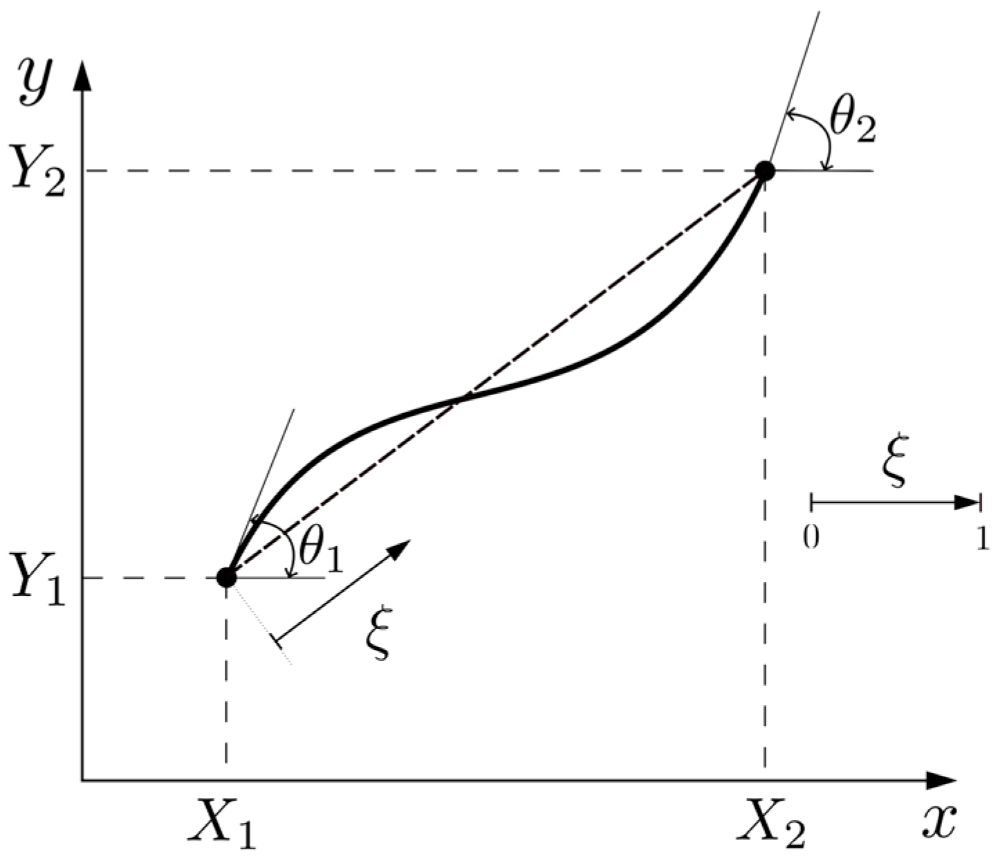
The positional finite element method formulation applied to the dynamic problems presented here is based on the works of Oliveira and Greco [35] and Fernandes et al. [36]. The finite element kinematics, described in terms of absolute coordinates ( X 1 ,   Y 1 ,   X 2 , Y 2 ) and the dimensionless parameter ξ (varying from 0 to 1), is presented in Figure 1.
The energy equilibrium of a mechanical system occurs if the input and output of energy are at balance. If there is some kind of dissipation, the total energy of the system changes over time. Thus, the functional of the total potential energy (Π) can be determined using the principle of virtual work, as follows:
Π = U + K C + K D W
where U represents the total strain energy (including plasticity and damage effects), K C represents kinetic energy, K D represents the physical damping term and W represents the potential energy of the external applied forces. These terms are expressed by
U = V u d V = V ε σ d ε d V
K C = V ρ 2 X ˙ 2 d V
K D = V c m ρ X X ˙ d V V X k c m ρ X X ¨ X ˙ d X k d V
W = q = 1 D o F P q X q
In the set of Equations (17)–(20), V is the element volume, c m is a damping coefficient proportional to mass, ρ is the element specific mass and P q is the force applied at a specific q degree of freedom (DoF). The stress tensor is represented by σ and the strain tensor is represented by ε . The mass matrix of the elements is considered discrete and the mass terms due to rotation are neglected.
Applying variational principles, it is possible to obtain the equilibrium configuration corresponding to the minimum functional energy as follows:
δ Π = 0
For variations regarding the q degrees of freedom, one has
δ Π = Π X q δ X q = 0
For variations regarding the q degrees of freedom ( q = 1 , 2 , , n g l ), one has
δ Π = Π X q δ X q = U X q + K C X q + K D X q W X q δ X q = 0
The Newton–Raphson iterative method, associated with the Newmark time marching procedure, is considered here, adopting the structure discretized by the nodal positions.
Equation (23) can be written in a compact form, as follows:
δ Π X q = g q X = 0
where g q X represents the vector of residues, g q , r X represents the Hessian matrix and X r represents the nodal position correction vector.
g q X = U , q + K C , q + K D , q + P q
g q , r X = U , q r
Thus, the discretized movement equation for an actual time instant ( t + Δ t ) is expressed by
Π X t + Δ t = U X t + Δ t F t + Δ t + M X ¨ t + Δ t + C X ˙ t + Δ t = 0
The Newmark time marching time integration is based here on elements’ absolute nodal positions, as follows:
X t + Δ t = X t + Δ t X ˙ t + Δ t 2 1 2 β X ¨ t + β X ¨ t + Δ t
X ˙ t + Δ t = X ˙ t + Δ t 1 γ X ¨ t + γ Δ t X ¨ t + Δ t
where γ and β are constants depending on the acceleration approximation used (here considered as γ = 0.5 and β = 0.25 ).
After the initial accelerations ( X ¨ 0 ) are evaluated, Equations (28) and (29) are replaced in Equation (27) given the following nonlinear dynamic equilibrium equation:
Π X t + Δ t = U X t + Δ t F t + Δ t + M β Δ t 2 X t + Δ t M D t + C E t + γ C β Δ t X t + Δ t γ Δ t C Q t = 0
where vectors D t and E t represent the contributions of the variables considered in the previous time instant t .
D t = X t β Δ t 2 + X ˙ t β Δ t + 1 2 β 1 X ¨ t
E t = X ˙ t + Δ t 1 γ X ¨ t
The Hessian matrix for dynamic problem is given by
g q , r X 2 Π X 2 t + Δ t = g X 0 = 2 U X 2 t + Δ t + M β Δ t 2 + γ C β Δ t

2.5. Flowchart of the Structure Integrity Analysis

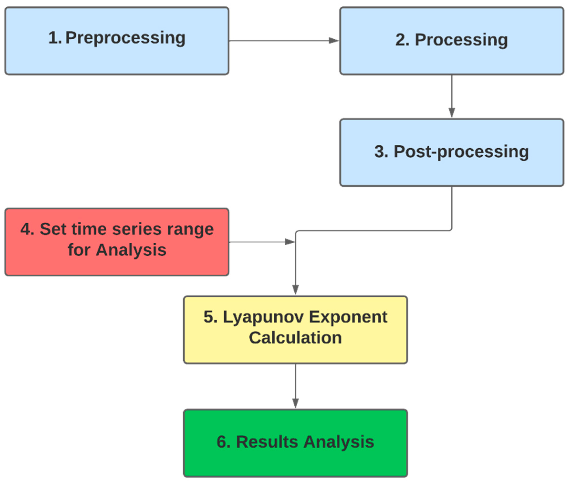
Figure 2 shows a flowchart with the steps taken during the integrity analysis of the frame structures, for example (1) in the preprocessing step, one defines the geometry, material model, boundary conditions, applied forces, time integration method and dynamic parameters; (2) the processing represents the solution of nonlinear dynamic equilibrium equations using the positional finite element method; (3) the post-processing of the structural analysis is the data processing for the visualization and analysis of results, for example, graph plotting, table creation, illustrations of equilibrium trajectory and deformed configuration, among others; (4) step 4 is when one sets the time series ranges for analysis, considering specific intervals of interest and the appropriate size to obtain accurate results; (5) the Lyapunov exponent calculation is performed by inserting time series of the nodal position into the nonlinear predictor algorithm; and (6) in the results analysis, one compares the maximum Lyapunov exponent from each selected range of the time series and investigates if the observation of the Lyapunov exponent is a reliable way of identifying structural degradation (instability, material damage, snap-through phenomena occurrence, etc.).
In the present study, steps 1, 2 and 3 consider the use of an original script of the positional finite element method implemented by the authors. However, once the method of assessing structural integrity is validated, one can use any finite element method commercial software. Another possibility is the use of experimental data; so, step 3 would use information acquired experimentally, recalling that as explained in the introduction, it is possible to use acceleration data instead of displacement data without a loss of accuracy.

3. Results

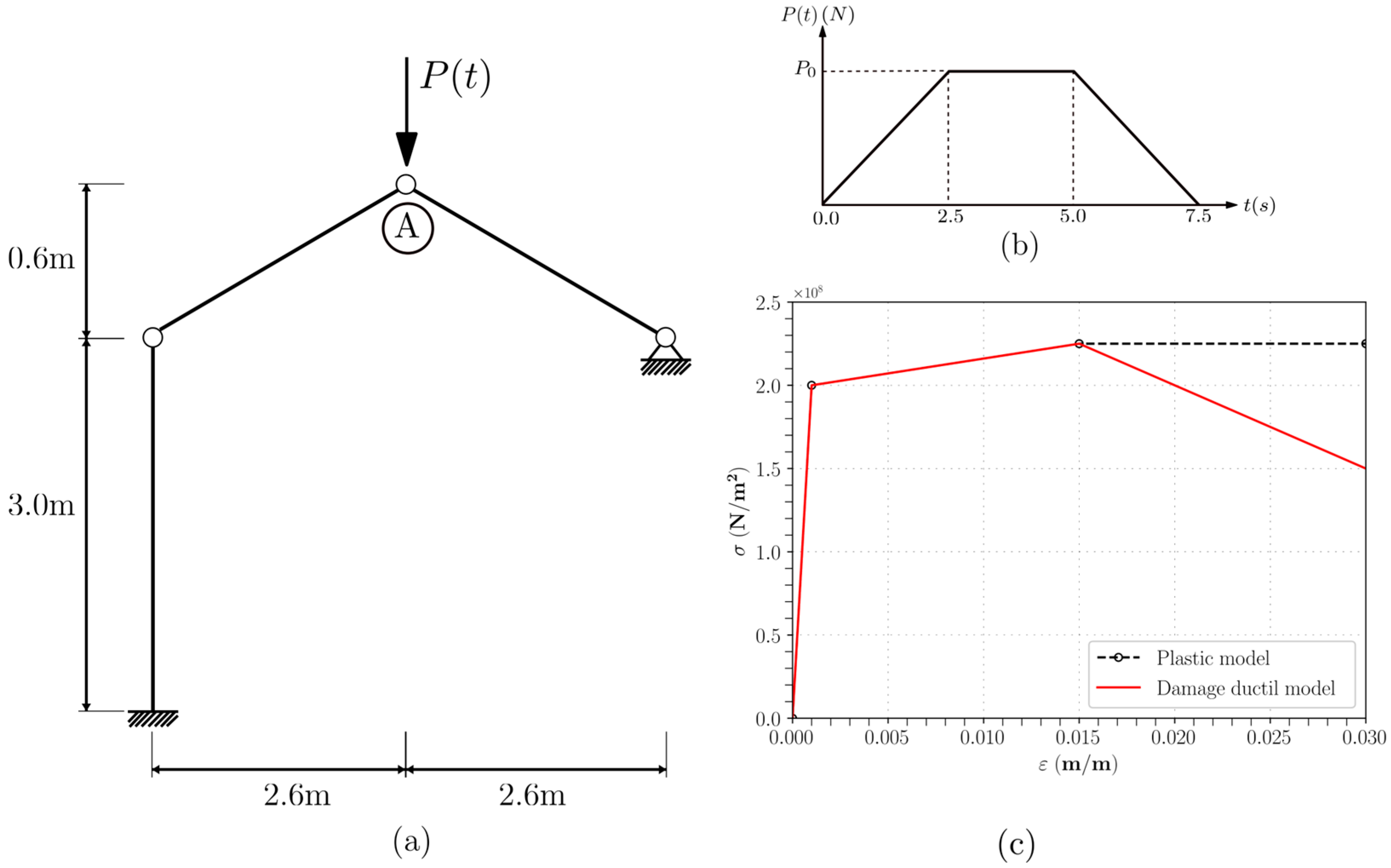
The numerical application consists of a framed structure with an upper section similar to a von Mises truss, as is shown in Figure 3. The modulus of elasticity is 200   G P (steel), the cross-sectional area of the bars is equal to 1.76 × 10 3   m 2 and the moment of inertia of the bars is equal to 1.04 × 10 6   m 4 for the column and equal to 2.59 × 10 7   m 4 for the other bars. The specific mass is equal to 7850   k g / m 3 and the damping factor considered is equal to 0.05. The parameters of the ductile damage model are a 1 p = 0.0 , a 2 p = 65.041 , a 3 p = 0.0 , ε d p = 0.004625 and D c = 0.33 . Regarding time integration, time increments of 0.0005 s and γ = 0.5 and β = 0.25 were adopted in the Newmark integration. The loading phases are presented in Figure 3b.
The chosen example is conceptual by nature, serving the purpose of illustrating the verification sequence and evaluating the applicability of the proposed methodology. Despite this, the developed algorithm can receive the design parameters of real structures as its input.
Three models were initially made with different meshes, considering four, six and eight elements per bar. The frequencies for the respective loops are shown in Table 1. In dynamic problems, excessive mesh refinement may not physically produce the best results, since high-order frequencies may spuriously influence the response. In general terms, the responses of all meshes were close, except in cases with inelasticity, in which six-element mesh achieved the expected responses from the physical point of view and over a longer analysis time. The other meshes studied failed in regard to this last consideration.
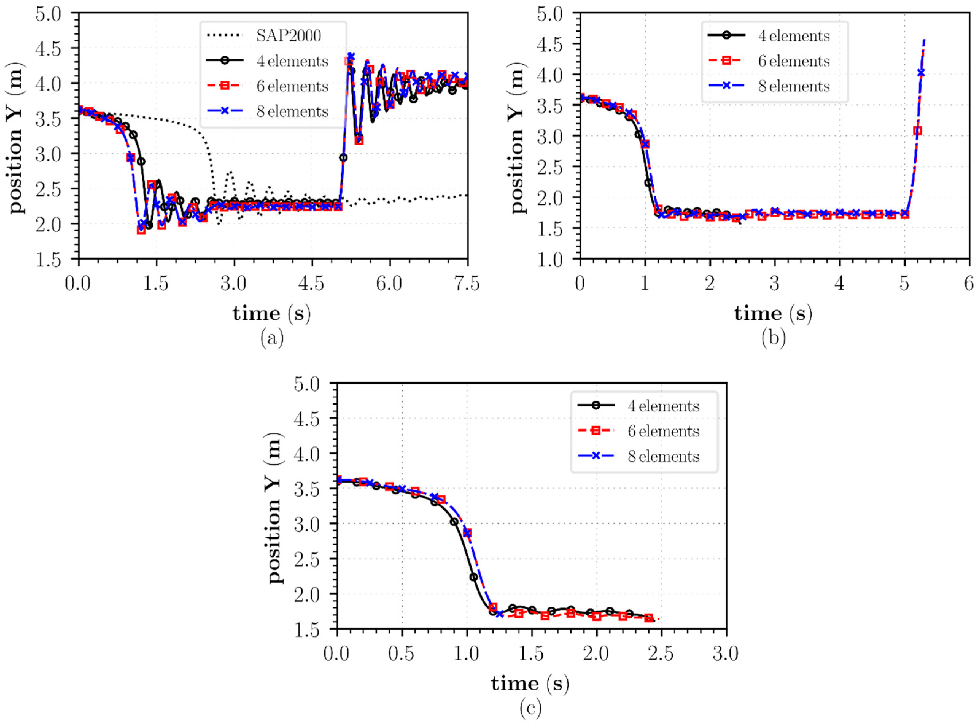
In Figure 4, the responses of each material model with the mentioned meshes are presented. It can be observed that there is a convergence of responses between meshes with six and four elements for the elastic response (Figure 4a) and the plastic response (Figure 4b). In the damage model (Figure 4c), the four-element and the six-element meshes present a longer-lasting response, but the responses slightly differ. Thus, the mesh with the longest period is the mesh with six elements, since in the plastic model the mesh with four elements presents a response only up to 2.46 s. There is also a discrepancy between the response presented by SAP2000 in the elastic model in relation to the responses of the present formulation. This difference can be explained, in theory, by the difference in the finite elements used by the SAP2000 and by the positional method. The data presented below were obtained considering the six-element mesh.
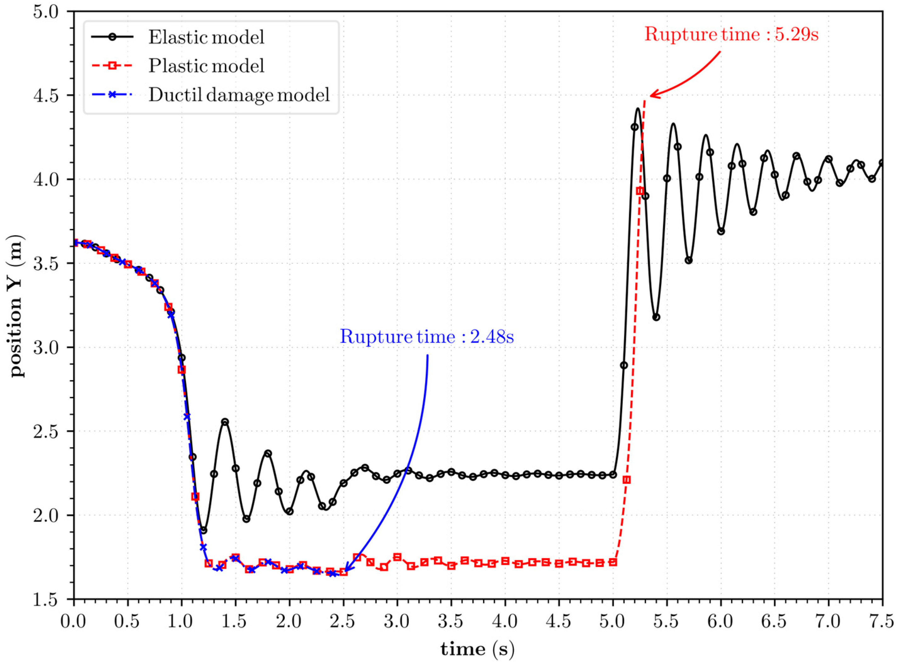
Figure 5 presents a comparison between responses for the six-element mesh of all material models. It can be noticed that there is an occurrence of snap-through in all models, but in the inelastic model the jump is more intense, taking node A up to approximately 1.6 m, while in the elastic model it approaches 1.8 m. In both models it occurs between 1.0 and 1.5 s. After the jump, oscillations of decreasing amplitude are observed in the elastic model, which cease around 3.0 s. This damping is observed practically instantaneously in the inelastic model after snap-through.
Around the time instant of 5.0 s, another leap occurs, which is due to the characteristic of the dynamic applied force. After this new jump, node A, in the elastic model, presents oscillations that tend to 4.0 m at the end of the analysis. The plastic model does not provide results until the end, since the base of the column undergoes plastification and the structure collapses at 5.29 s. Structure failure in the ductile damage model is much more premature, occurring at 2.48 s of analysis. Due to the constitutive curve used in the example and the geometric characteristics of the structure, no substantial differences can be noticed between the responses of the inelastic models, except for the premature break in the damage model. It should be noted that the first plastification takes 0.59 s for analysis, while the first degradation takes 1.19 s.
Considering the acceleration responses, presented in Figure 6, a slightly more accentuated tendency for the accelerations to decrease can be seen in the damage model in relation to the plastic model. It is interesting to note how the acceleration presents jumps; in the plastic and damage model, they are in the order of 800   m / s 2 , eight times greater than the elastic model. Near the second jump, an increase in acceleration is again observed, reaching 900   m / s 2 in the plastic model, again higher than the elastic model, which presents a maximum acceleration of 600   m / s 2 .
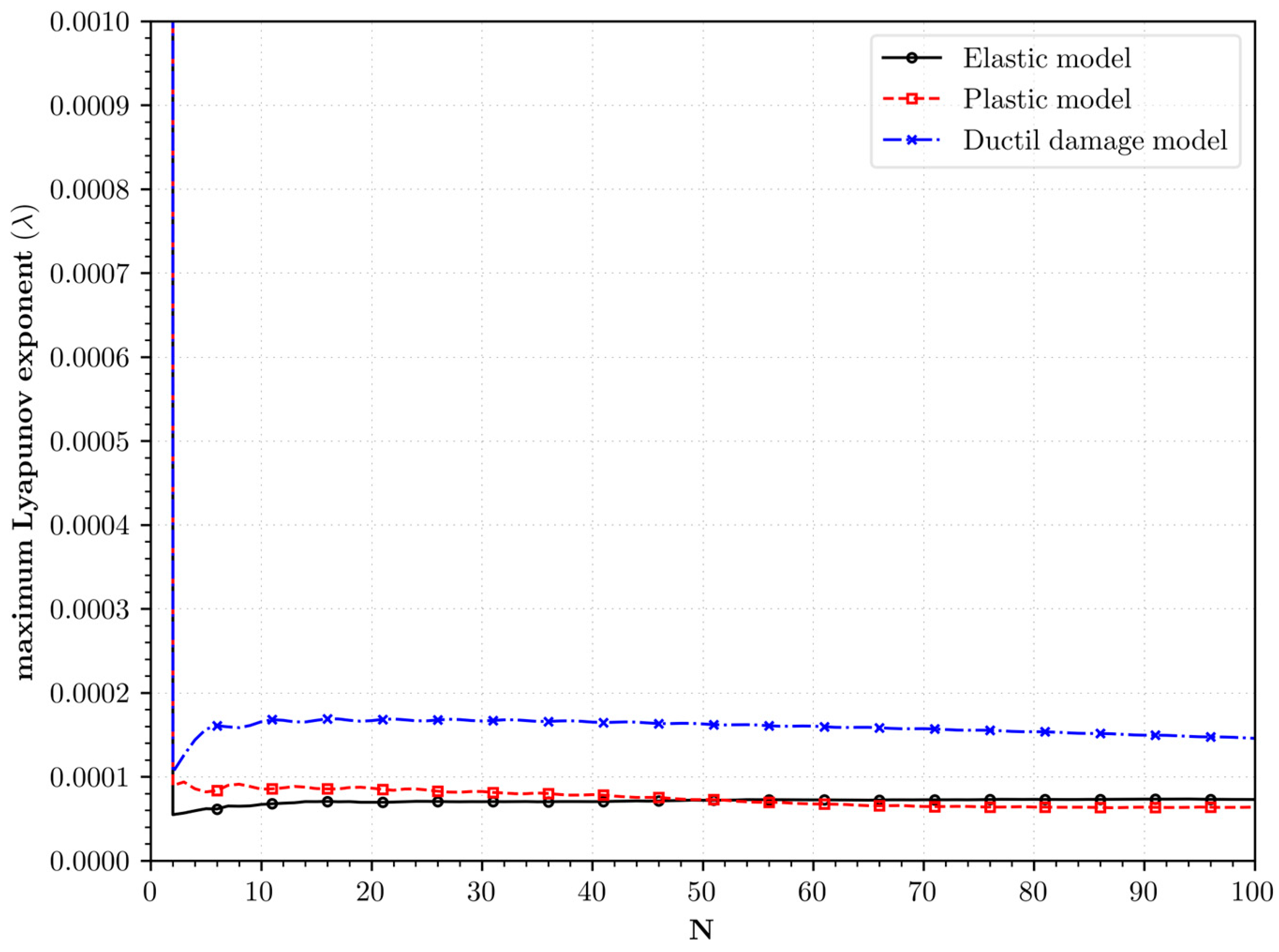
To obtain the largest Lyapunov exponent, three sets of time series were adopted, with the first set between 0 s and 1.3 s, the second, from 1.3 s to 5.0 s, and the third, from 5.0 s to the end of the analysis. Notably, the ductile damage model only provided results for the first and second spans.
Figure 7 shows the convergence of the highest Lyapunov exponent, where N is the number of points close to the analysis point for the first analysis set. Note the convergence of λ for the elastic model in the order of 0.01. The inelastic models, however, present λ tending to 0.001.
For the second set of data, from 1.3 s to 5 s, there is a certain stabilization of the structure at the new position after the snap presented in Figure 8, as λ is detected for all the models, which tends to 5 × 10 5 .
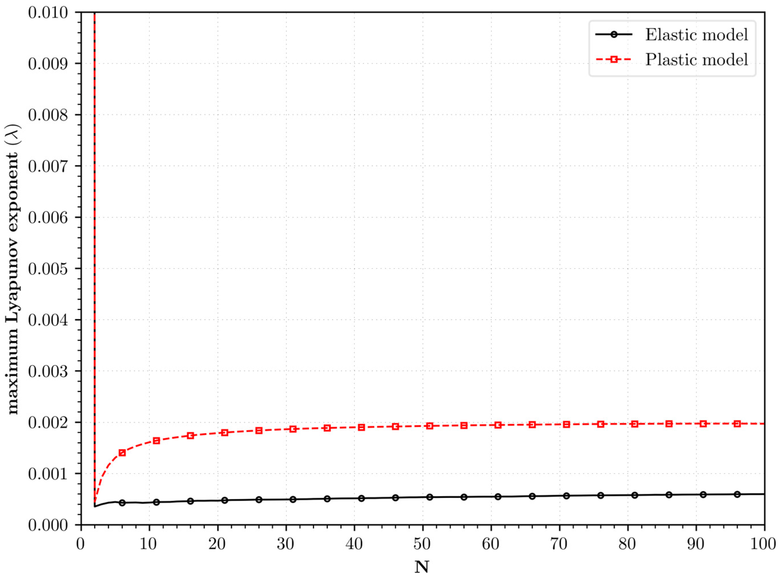
Finally, in the last part of the analysis, only the elastic and plastic models provide results, justifying the absence of the damage model in Figure 9. For the elastic model, λ tends to 5 × 10 4 , indicating the stabilization that occurs in the elastic model despite the jump. The plastic model, however, tends towards a high Lyapunov exponent of 0.002, justified by the sudden break in the jump.

4. Discussion

The responses of the inelastic models used in this article were theoretically consistent, both presenting energy dissipation characterized by a decrease in oscillation. The loss of stiffness was also observed, due to ruptures before the end of the analysis time, as well as more flexible responses when compared to the elastic model. Failure in cross-sections with low levels of oscillation or increased stress in the structure highlights the structural response of the damage model, characterized by a strong decrease in material stiffness. Thus, such models are useful for describing the behavior of structures under strong non-linearities that may occur in real situations such as buildings, bridges, transmission towers, industrial structures or structures in general in a situation of progressive collapse.
In addition to the presented numerical results, phase figures related to the position and velocity of the top central node are presented in Figure 10. The analyses of the results of the elastic model, elastoplastic model and ductile damage model are also presented. The initial vertical position is the same for three analyses, i.e., 3.6   m (with null velocity). It is clearly possible to note two point attractors in the elastic response (the first one at the left and the second one at the right). Two dynamic snap-throughs are noted (initial position to the left attractor and left attractor to the right attractor). For elastoplastic response, only the left attractor is noted, but two snap-throughs are observed. For the ductile damage model, only one attractor and one snap-through are noted. Inelastic models present smaller oscillation amplitudes and more stable trajectories on phase figures. For the modeling of realistic building structures, inelastic effects analyses are advisable. These effects can mask instability identification.
Phase figures related to the position and acceleration of the top central node are presented in Figure 11. Again, analyses results of the elastic model, elastoplastic model and ductile damage model are presented. But, contrary to the velocity phase figure, trajectories, snap-through and attractors are not so evident. Only for the ductile damage model it is possible to note instabilities when central node position reaches the position close to 2.5   m .
The use of Lyapunov exponents in monitoring the integrity of the analyzed structure has been proven to be promising, since it was able to detect the occurrence of the destabilization of the structure with the dynamic jump and the presence of material failures by means of a comparison between the responses of undamaged/stabilized and damaged/unstabilized structures. However, as pointed out by the technical literature on the subject [18], it is not possible to differentiate the phenomena just by observing the maximum Lyapunov exponent, leaving this level of detail to other essays/analyses. The use of only one time series is a characteristic to be highlighted in the technique for obtaining the Lyapunov exponent via the non-linear predictor, decreasing the computational cost and analysis time. Thus, a limitation that must be pointed out is the absence of negative exponents, making it difficult to immediately detect any structural failure, thus requiring an additional step of analysis since comparison with other response excerpts is necessary.
The chosen numerical example has different levels of damage in all elements (global), as well local damage next to the column base. Moreover, due to initial/boundary conditions, there occurs a dynamic snap-through depending on the considered constitutive model (elastic, elastoplastic or elastoplastic with damage).

Possible Directions for Future Studies

The presented methodology to assess structural integrity using the Lyapunov exponents is compatible with any damage model. The FLHB ductile-damage model used here has some restrictions in its applicability to concrete structures. It can be used only in situations that involve pure tensile or pure compressive loading, for instance. Thus, the next step of the research is to include a damage model capable of simulating the responses in brittle materials in a more general manner. One of the first options for concrete modeling is to use the concrete damaged plasticity (CDP) model [37]. The CDP is a modification of the Drucker–Prager model and considers the degradation of the elastic stiffness induced by plastic deformation, both for tensile stresses and for compressive stresses.
A promising application of the presented methodology is its use with experimental data instead of the data acquired, simulating a numerical example. Now that the methodology has shown itself capable of verifying the structural integrity, the practical use with experimental data is an interesting application, remembering that, as explained in the introduction, one can use data collected from accelerometers installed in real structures. As an example, Toloue et al. [38] used accelerometers to assess the damage of aluminum spatial frames. The authors used the damage load vectors (DLV) method in association with the application of the Markov matrix to the noisy accelerometer data, enabling the exclusive inclusion of the most useful signals.
Another possible work to be conducted is the comparison of the presented method, which uses the Lyapunov coefficients, with other methods of structural integrity verification. A comparison of Lyapunov exponent analysis with the evolution of damage indexes, as developed by Park and Ang [39] and applied by Karayannis and Goliath [40] for studying the structural performance parameters of concrete structures strengthened with carbon fiber reinforced, is a good example.
Finally, reliability and robustness analyses of the methodology should be performed in future studies, i.e., to assess the sensitivity to changes in input parameters, such as material properties and loading conditions.

5. Conclusions

This article presents a methodology, based on the use of Lyapunov exponents, to assess stability and structural integrity. A frame structure was used as numerical example to illustrate the applicability of the methodology. The structural analysis performed integrated the positional finite element method to address geometric nonlinearity, and the isotropic elastoplastic model together with the recently developed FLHB damage model were used to evaluate material nonlinearities. The equilibrium trajectories obtained with and without the consideration of material nonlinearities were examined, and the relevant differences revealed through a qualitative and quantitative analysis demonstrated the importance of using robust simulations that consider the nonlinearities.
An important feature of the methodology is the non-linear predictor that needs a single data series, which proved to be an efficient technique for obtaining the Lyapunov exponents. This consists of an important result because it facilitates the applicability of the presented methodology due to its lower computational cost.
The results obtained through the application of the proposed methodology showed that it is possible to identify the loss of structural stiffness, even if it is related only to stability or if it involves physical nonlinearity phenomena such as plastification and damage. It can also be concluded that the Lyapunov exponents can be used as indicative parameters of structural integrity, as their analysis was able to detect the occurrence of the destabilization of the structure with the dynamic jump and the presence of material failures. Overall, the methodology presented here to monitor structural integrity was shown to be a promising alternative.
Author Contributions

Conceptualization, G.B.B., W.L.F., M.G. and D.H.N.P.; methodology, G.B.B., W.L.F., M.G. and D.H.N.P.; software, G.B.B., W.L.F. and M.G.; validation, G.B.B., W.L.F. and D.H.N.P.; investigation, G.B.B. and W.L.F.; resources, G.B.B., W.L.F. and M.G.; data curation, G.B.B., W.L.F. and M.G.; writing—original draft preparation, G.B.B., M.G. and D.H.N.P.; writing—review and editing, G.B.B., W.L.F., M.G. and D.H.N.P.; supervision, M.G.; project administration, M.G.; funding acquisition, M.G. All authors have read and agreed to the published version of the manuscript.

Funding

This research was funded by Fundação de Amparo à Pesquisa do Estado de Minas Gerais (FAPEMIG), grant number PPM-00444-18, and Conselho Nacional de Desenvolvimento Científico e Tecnológico (CNPq), grant number 302119/2022-1.

Data Availability Statement

All data used and materials developed in this research are available on request.

Conflicts of Interest

The authors declare no conflict of interest.

References

  1. Wang, K.; Kajita, Y.; Yang, Y. Bayesian RC-Frame Finite Element Model Updating and Damage Estimation Using Nested Sampling with Nonlinear Time History. Buildings 2023, 13, 1281. [Google Scholar] [CrossRef]
  2. Buka-Vaivade, K.; Kurtenoks, V.; Serdjuks, D. Non-Destructive Damage Detection of Structural Joint by Coaxial Correlation Method in 6D Space. Buildings 2023, 13, 1151. [Google Scholar] [CrossRef]
  3. Guo, Z.; Bu, J.; Zhang, J.; Cao, W.; Huang, X. Theoretical and Numerical Investigation of Damage Sensitivity of Steel–Concrete Composite Beam Bridges. Buildings 2023, 13, 1109. [Google Scholar] [CrossRef]
  4. Dyer, A.S.; Zaengle, D.; Nelson, J.R.; Duran, R.; Wenzlick, M.; Wingo, P.C.; Bauer, J.R.; Rose, K.; Romeo, L. Applied machine learning model comparison: Predicting offshore platform integrity with gradient boosting algorithms and neural networks. Mar. Struct. 2022, 83, 103152. [Google Scholar] [CrossRef]
  5. Sarmadi, H. Investigation of Machine Learning Methods for Structural Safety Assessment under Variability in Data: Comparative Studies and New Approaches. J. Perform. Constr. Facil. 2021, 35, 04021090. [Google Scholar] [CrossRef]
  6. Pishro, A.A.; Zhang, Z.; Pishro, M.A.; Liu, W.; Zhang, L.; Yang, Q. Structural Performance of EB-FRP-Strengthened RC T-Beams Subjected to Combined Torsion and Shear Using ANN. Materials 2022, 15, 4852. [Google Scholar] [CrossRef] [PubMed]
  7. Pishro, A.A.; Zhang, Z.; Pishro, M.A.; Xiong, F.; Zhang, L.; Yang, Q.; Matlan, S.J. UHPC-PINN-parallel micro element system for the local bond stress–slip model subjected to monotonic loading. Structures 2022, 46, 570–597. [Google Scholar] [CrossRef]
  8. Wolf, A.; Swift, J.B.; Swinney, H.L.; Vastano, J.A. Determining Lyapunov exponents from a time series. Phys. D Nonlinear Phenom. 1985, 16, 285–317. [Google Scholar] [CrossRef] [Green Version]
  9. Sano, M.; Sawada, Y. Measurement of the Lyapunov Spectrum from a Chaotic Time Series. Phys. Rev. Lett. 1985, 55, 1082–1085. [Google Scholar] [CrossRef]
  10. Briggs, K. An improved method for estimating Liapunov exponents of chaotic time series. Phys. Lett. A 1990, 151, 27–32. [Google Scholar] [CrossRef]
  11. Abarbanel, H.D.I.; Brown, R.; Kennel, M.B. Variation of Lyapunov exponents on a strange attractor. J. Nonlinear Sci. 1991, 1, 175–199. [Google Scholar] [CrossRef]
  12. Dingwell, J.B. Lyapunov Exponents. In Wiley Encyclopedia of Biomedical Engineering; John Wiley & Sons, Ltd.: Hoboken, NJ, USA, 2006. [Google Scholar] [CrossRef]
  13. Sprott, J.C. Chaos and Time-Series Analysis; Oxford University Press: Oxford, UK; New York, NY, USA, 2003. [Google Scholar]
  14. Cardoso, V.; Miranda, A.S.; Berti, E.; Witek, H.; Zanchin, V.T. Geodesic stability, Lyapunov exponents, and quasinormal modes. Phys. Rev. D 2009, 79, 064016. [Google Scholar] [CrossRef] [Green Version]
  15. Vannitsem, S. Predictability of large-scale atmospheric motions: Lyapunov exponents and error dynamics. Chaos Interdiscip. J. Nonlinear Sci. 2017, 27, 032101. [Google Scholar] [CrossRef] [Green Version]
  16. Fernandes, W.L. Parametric Analysis of the Instability of Slender Plane Lattice Structures with Geometrically Nonlinear Dynamic Behavior by Positional Finite Element Method. In Portuguese. Ph.D. Thesis, Federal University of Minas Gerais, Belo Horizonte, Brazil, 2022. (In Portuguese). [Google Scholar]
  17. Barbosa, G.B.; Fernandes, W.L.; Greco, M. Chaotic Behavior Analysis of Two-Bar Trusses under Inelastic Effects through Lyapunov Exponents. In Proceedings of the XLII Ibero-Latin-American Congress on Computational Methods in Engineering and III Pan-American Congress on Computational Mechanics, Rio de Janeiro, Brazil, 13–16 November 2023; Available online: https://cilamce.com.br/anais/arearestrita/apresentacoes/235/9191.pdf (accessed on 4 July 2023).
  18. Worden, K.; Farrar, C.R.; Haywood, J.; Todd, M. A review of nonlinear dynamics applications to structural health monitoring. Struct. Control Health Monit. 2008, 15, 540–567. [Google Scholar] [CrossRef]
  19. Casciati, F.; Casciati, S. Structural health monitoring by Lyapunov exponents of non-linear time series. Struct. Control. Health Monit. Bull. ACS 2006, 13, 132–146. [Google Scholar] [CrossRef]
  20. Jin, S.; Jalinoos, F.; Livingston, R. Application of Chaos Theory Analysis to Accelerometer Data in Structural Health Monitoring of Highway Bridges. In SMT—ASNT Conference; ASNT: Buffalo, NY, USA, 2008. [Google Scholar]
  21. Zhou, J.; Chen, Y.; Yin, L. Lyapunov Exponent Analysis On Real-Time Monitoring Information of Extractive Structure Health Based on Chaos Time Sequence. Intell. Autom. Soft Comput. 2010, 16, 737–745. [Google Scholar] [CrossRef]
  22. Rai, A.; Kim, J.-M. A novel health indicator based on the Lyapunov exponent, a probabilistic self-organizing map, and the Gini-Simpson index for calculating the RUL of bearings. Measurement 2020, 164, 108002. [Google Scholar] [CrossRef]
  23. Felipe, T.R.; Leonel, E.D.; Haach, V.G.; Beck, A.T. A comprehensive ductile damage model for 3D truss structures. Int. J. Non-linear Mech. 2019, 112, 13–24. [Google Scholar] [CrossRef]
  24. Hilborn, R. Chaos and Nonlinear Dynamics: An Introduction for Scientists and Engineers, 2nd ed.; Oxford University Press: Oxford, UK; New York, NY, USA, 2001. [Google Scholar]
  25. Strogatz, S.H. Nonlinear Dynamics And Chaos: With Applications To Physics, Biology, Chemistry, And Engineering, 1st ed.; Westview Press: Cambridge, MA, USA, 2001. [Google Scholar]
  26. Souza Neto, E.A.; Peric, D.; Owen, D.R.J. Computational Methods for Plasticity: Theory and Applications, 1st ed.; Wiley: Chichester, West Sussex, UK, 2008. [Google Scholar]
  27. Felipe, T.R.C. Análise Mecânica e Probabilística de Estruturas Treliçadas Sujeitas ao Colapso Progressivo. 2019. Available online: https://www.teses.usp.br/teses/disponiveis/18/18134/tde-26112019-125059/publico/DO2019_TulioRaunyrCandidoFelipe.pdf (accessed on 4 July 2023). (In Portuguese).
  28. Lemaitre, J. A Course on Damage Mechanics, 2nd ed.; Springer: Berlin, Germany; New York, NY, USA, 1996. [Google Scholar]
  29. Chaves, E.W.V. Notes on Continuum Mechanics; 2013a edição; Springer: Berlin/Heidelberg, Germany, 2013. [Google Scholar] [CrossRef]
  30. Owen, D.R.J.; Peric, D.; Neto, E.A.d.S. Computational Methods for Plasticity: Theory and Applications., 1st ed.; John Wiley & Sons Inc.: Chichester, West Sussex, UK, 2008. [Google Scholar]
  31. Zhang, W.; Cai, Y. Review of Damage Mechanics. In Continuum Damage Mechanics and Numerical Applications Advanced Topics in Science and Technology in China; Zhang, W., Cai, Y., Eds.; Springer: Berlin/Heidelberg, Germany, 2010; pp. 15–57. [Google Scholar] [CrossRef]
  32. Kachanov, L.M. Time of the Rupture Process under Creep Condition. Izv Akad Nauk SSSR Otd Tekhn Nauk 1958, 8, 26–31. [Google Scholar]
  33. Lemaitre, J. Coupled elasto-plasticity and damage constitutive equations. Comput. Methods Appl. Mech. Eng. 1985, 51, 31–49. [Google Scholar] [CrossRef]
  34. Felipe, T.R.; Beck, A.T. Dynamic analysis of failure paths of truss structures: Benchmark examples including material degradation. Mech. Syst. Signal Process 2021, 158, 107767. [Google Scholar] [CrossRef]
  35. de Oliveira, F.M.; Greco, M. Nonlinear dynamic analysis of beams with layered cross sections under moving masses. J. Braz. Soc. Mech. Sci. Eng. 2015, 37, 451–462. [Google Scholar] [CrossRef]
  36. Fernandes, W.L.; Barbosa, G.B.; Greco, M.; Silveira, R.A.D.M. Comparison between recent implicit time integration methods with frequency dissipation for nonlinear structural applications. Lat. Am. J. Solids Struct. 2022, 19, e441. [Google Scholar] [CrossRef]
  37. Lubliner, J.; Oliver, J.; Oller, S.; Oñate, E. A plastic-damage model for concrete. Int. J. Solids Struct. 1989, 25, 299–326. [Google Scholar] [CrossRef]
  38. Toloue, I.; Liew, M.S.; Harahap, I.S.H.; Lee, H.E. Damage detection in frame structures using noisy accelerometers and Damage Load Vectors (DLV). Sci. Iran. 2020, 27, 1776–1785. [Google Scholar] [CrossRef] [Green Version]
  39. Park, Y.-J.; Ang, A.H.-S. Mechanistic Seismic Damage Model for Reinforced Concrete. J. Struct. Eng. 1985, 111, 722–739. [Google Scholar] [CrossRef]
  40. Karayannis, C.G.; Golias, E. Full-scale experimental testing of RC beam-column joints strengthened using CFRP ropes as external reinforcement. Eng. Struct. 2022, 250, 113305. [Google Scholar] [CrossRef]
Figure 1. Finite element kinematics described in terms of absolute coordinates.
Buildings 13 01802 g001
Figure 2. Flowchart of the methodology.
Buildings 13 01802 g002
Figure 3. Example data: (a) structural frame; (b) applied dynamic force; (c) constitutive laws.
Buildings 13 01802 g003
Figure 4. Top vertical node position for: (a) elastic model; (b) elastoplastic model; (c) ductile damage model.
Buildings 13 01802 g004
Figure 5. Top vertical node positions along time for different models.
Buildings 13 01802 g005
Figure 6. Top vertical accelerations over time for different models.
Buildings 13 01802 g006
Figure 7. Convergence of maximum Lyapunov exponents for time interval 0.0 s to 1.3 s.
Buildings 13 01802 g007
Figure 8. Convergence of maximum Lyapunov exponents for time interval 1.3 s to 5.0 s.
Buildings 13 01802 g008
Figure 9. Convergence of maximum Lyapunov exponents for time interval 5.0 s to 7.5 s.
Buildings 13 01802 g009
Figure 10. Top vertical node phase figure for position and velocity: (a) elastic model; (b) elastoplastic model; (c) ductile damage model.
Buildings 13 01802 g010
Figure 11. Top vertical node phase figure for position and acceleration: (a) elastic model; (b) elastoplastic model; (c) ductile damage model.
Buildings 13 01802 g011
Table 1. Fundamental frequency considering different finite element meshes.
Finite Elements per BarFundamental Frequency
Positional FEMSAP2000
42.375502.364
62.013162.382
82.018612.389
Disclaimer/Publisher’s Note: The statements, opinions and data contained in all publications are solely those of the individual author(s) and contributor(s) and not of MDPI and/or the editor(s). MDPI and/or the editor(s) disclaim responsibility for any injury to people or property resulting from any ideas, methods, instructions or products referred to in the content.