Abstract
This study explores the utilization of the Relevance Vector Machine (RVM) model, optimized using the Sparrow Search Algorithm (SSA), Simulate Anneal Arithmetic (SAA), Particle Swarm Optimization (PSO), and Bayesian Optimization Algorithm (BOP), to construct an energy dissipation model for public buildings in Wuhan City. Energy consumption data and influential factors were collected from 100 public buildings, yielding 15 input variables, including building area, personnel density, and supply air temperature. Energy dissipation served as the output scalar indicator. Through correlation analysis between input and output variables, it was found that building area, personnel density, and supply air temperature significantly impact energy dissipation in public buildings. Principal component analysis (PCA) was employed for data dimensionality reduction, selecting seven main influential factors along with energy dissipation values as the dataset for the predictive model. The BOP-RVM model showed superior performance in terms of R2 (0.9523), r (0.9761), and low RMSE (5.3894) and SI (0.056). These findings hold substantial practical value for accurately predicting building energy consumption and formulating effective energy management strategies.
1. Introduction
Building energy consumption has become an important research field, given the growing global energy demand and increasing concern about environmental sustainability. As building energy consumption accounts for a considerable proportion of global energy consumption, accurate prediction and management of building energy consumption are crucial for energy conservation and environmental protection [1,2,3]. However, due to the influence of multiple complex factors that go into building energy consumption, traditional prediction models based on rules and statistical methods often have certain limitations. As a response to these limitations, recent advancements in technology have brought forth more effective solutions.
In recent years, the rapid development of machine learning technology has provided new possibilities for solving the problem of building energy consumption prediction. Machine learning, a subset of artificial intelligence, uses sophisticated computer algorithms and models to learn patterns from large volumes of data, enabling more precise predictions or decisions. By analyzing and learning from vast sets of building energy consumption data, machine learning models can automatically discover complex patterns and associations that traditional models may miss, thereby enhancing the accuracy of future energy consumption predictions. Zhao et al. [4] divided building energy consumption modeling and prediction methods into engineering, statistical, and artificial intelligence methods. They proposed that the most widely used method is artificial intelligence. Amasyali et al. [5] believed that building energy consumption prediction mainly adopts two methods: the physical model method and the data-driven method, and pointed out that the data-driven method has a super learning ability and can better solve complex problems in building energy consumption prediction. Wang et al. [6] divided building energy consumption prediction methods into engineering, artificial intelligence, and hybrid methods and proposed to select the appropriate artificial intelligence method model for building energy consumption prediction, which will obtain a higher prediction accuracy. Foucquier et al. [7] studied building energy consumption from three models—the white box, gray box, and black box—and pointed out that the black box model has a faster calculation speed and shorter prediction time. In order to reduce the redundant factors of building energy consumption, Lei et al. [8] used the deep learning method to find out the influence of key factors on building energy consumption. Taking the key factors as the input of the deep neural network and the building energy consumption as the output, the accurate prediction of the building energy consumption is realized. In summary, compared with the traditional methods, the machine learning model has more substantial flexibility and generalization ability and can adapt to the energy consumption prediction requirements under different building types and environmental conditions [9,10,11].
While machine learning has yielded impressive results across various fields, applying it to building energy consumption prediction presents unique challenges [12,13,14]. Firstly, building energy consumption is influenced by numerous factors, such as indoor and outdoor temperatures, humidity, wind speed, building structure, and equipment. These factors have complex nonlinear relationships, making the selection of appropriate input variables and the establishment of an accurate model structure significantly challenging. Secondly, data related to building energy consumption typically exhibit high dimensionality and large sample sizes [15,16]. Processing and analyzing these data are daunting tasks. Additionally, the data often contain a certain degree of noise and uncertainty, emphasizing the necessity of enhancing the robustness and predictive accuracy of the model [17,18,19].
This study aims to address the challenges in predicting energy consumption in buildings by constructing a building energy consumption prediction model based on machine learning methods. The objective is to enhance the understanding and prediction accuracy of building energy consumption. The model is developed by collecting energy consumption data and related factors over a period of one year from 100 civil public buildings in Wuhan.
Fifteen key input variables are selected, all of which have a significant impact on energy consumption. For instance, indoor and outdoor temperatures, relative humidity, and wind speed influence the heating or cooling needs of a building, while the number of floors, building area, and personnel density can increase overall energy demand. Other variables include the building aspect ratio, roof heat transfer coefficient, lighting power density, per capita fresh air volume, air supply temperature, fan efficiency, and pump efficiency [20,21,22]. These factors, intricately connected to building energy consumption, provide sufficient information to predict it accurately [23,24]. The inclusion of these comprehensive variables aims to address the inherent complexity in predicting building energy consumption, thereby enhancing the accuracy, effectiveness, and efficiency of the model.
In order to deal with high-dimensional and extensive sample data, this study introduces the principal component analysis (PCA) method for data dimensionality reduction. PCA analysis identifies the main features and change patterns in the data, thereby reducing the number of input variables, simplifying the complexity of the model, and improving the prediction effect. After implementing PCA for data simplification, this study proceeds with the use of several commonly used machine learning models to predict building energy consumption, including Relevance Vector Machine (RVM), Bayesian Optimization-based RVM (BOP-RVM), Simulated Annealing Algorithm-based RVM (SAA-RVM), and Particle Swarm Optimization-based RVM (PSO-RVM). By comparing the performance of these models using key performance indicators such as determination coefficient, linear correlation value, and root mean square error, a more comprehensive evaluation of their predictive ability and applicability can be conducted. The goal is to identify the most effective model for predicting building energy consumption. The aim of this study is to provide a method for accurately predicting building energy consumption and establish a scientific basis for energy management and optimization. By constructing a building energy consumption prediction model based on machine learning, we can better understand the changing rules of building energy consumption and formulate corresponding energy-saving measures and strategies. Understanding these changes is critical for sustainable building development, as it aids in reducing energy waste and environmental pollution.
2. Machine Learning Algorithm Model
2.1. Relevance Vector Machine
The Relevance Vector Machine (RVM) is a probabilistic model for data features that operates within a Bayesian framework. This model can be utilized for regression prediction analysis. Through training with data, RVM can generate a sparse model that excludes some non-relevant data points, consequently reducing computational requirements.
The fundamental principle of Relevance Vector Machine (RVM) involves the introduction of an independent prior distribution to the model’s parameters, followed by the derivation of the posterior probability via Bayes’ theorem. This prior distribution takes the form of a Gaussian distribution centered around zero, where the variance is an unknown parameter. The value of this parameter significantly impacts the sparsity of the outcome, thereby necessitating its estimation via iterative optimization. More specifically, RVM utilizes a technique known as Automatic Relevance Determination (ARD) to facilitate this optimization process.
While the RVM model shares a similar form with Support Vector Machines (SVM), the learning strategies employed differ. SVM uses convex optimization techniques when solving optimization problems, striving for a global optimal solution. In contrast, RVM opts for iterative optimization. Although this might only yield a local optimum, the Bayesian framework characteristic of RVM allows for the estimation of prediction result probabilities.
2.2. Sparrow Search Algorithm
The Sparrow Search Algorithm (SSA) is a recent swarm intelligence optimization algorithm, introduced in 2020. Its design draws inspiration from the foraging and anti-predatory behavior of sparrows. During foraging activities, sparrows segregate themselves into two groups: discoverers (explorers) and participants (followers). The role of discoverers lies in locating food within their surroundings and providing foraging zones and directions for the sparrow community. Participants, on the other hand, rely on the discoveries of the explorers to gather food. Sparrows typically employ two key behavioral strategies to secure food: the finder strategy and the joiner strategy. The sparrow community keeps a vigilant watch on the activities of fellow members, and those identified as attackers vie with high-intake peers for food resources, thereby escalating their rate of predation. Moreover, sparrows enact anti-predatory strategies when they perceive threats, showcasing their adaptability and survival instinct [25,26].
2.3. Simulate Anneal Arithmetic
Simulated Annealing Algorithm (SAA) is a probabilistic technique employed to locate the optimal solution to a problem within a broad search space. The concept of simulated annealing originates from the metallurgical term “annealing”. In metallurgy, annealing refers to a process in which a material is heated and then cooled at a specific rate to enlarge the size of the grains and minimize defects in the crystal lattice. Atoms within the material initially reside in positions where internal energy achieves a local minimum. Upon heating, energy increases, prompting particles to abandon their original positions and randomly relocate elsewhere. The slow cooling rate in annealing allows particles to potentially discover positions with lower internal energy than before.
2.4. Particle Swarm Optimization
Particle Swarm Optimization (PSO) is a computational method for global optimization that simulates social behavior of bird flocks or fish schools. The fundamental idea underpinning PSO is as follows: within the search space, a swarm of particles is flying, each of which represents a potential solution, i.e., a point within this space. Every particle possesses a speed, dictating where it will venture next, and a fitness value, signifying the quality of its solution. These particles adjust their flight direction and speed based on their personal best historical position and the overall swarm’s best historical position, facilitating the search for superior solutions. The steps of the Particle Swarm Optimization algorithm are as follows:
Step 1. Initialization: randomly generate a swarm of particles, including their respective positions and speeds.
Step 2. Evaluation: compute the fitness value of each particle.
Step 3. Update: each particle updates its speed and position based on its personal best historical position and the swarm’s best historical position.
Step 4. Termination: If termination conditions are met (for instance, reaching the maximum number of iterations, or finding a solution that meets the required criteria), halt the algorithm; otherwise, return to step 2.
2.5. Bayesian Optimization
Bayesian Optimization Algorithm (BOP) is widely used in the automatic optimization of hyperparameters. Compared with traditional optimization algorithms, such as grid search and random optimization, Bayesian optimization algorithm can make full use of the searched information and update the hyperparameters on this basis, which avoids the search of a large number of invalid hyperparameter spaces. Therefore, the Bayesian optimization algorithm has higher search efficiency and stronger optimization ability.
In order to describe the relationship between the hyperparameter x and the objective function y(x), the Gaussian process surrogate model is established. Set up the searched information base , the Gaussian process proxy model can be expressed as:
where GP(*) is a Gaussian process and k(*) is a covariance function.
A common covariance function is denoted as:
The Gaussian process surrogate model can predict the objective function under any hyperparameters. In order to determine the next set of hyperparameters to be evaluated, the acquisition function is constructed on the prediction mean and prediction standard deviation of the Gaussian process surrogate model, and the acquisition function is maximized. PI(x), EI(x), and UCB(x)/LCB(x) are three commonly used acquisition functions defined as:
In the formula: Φ(·) is the standard normal distribution cumulative distribution function; μ(x) and σ(x) are the prediction mean and prediction standard deviation of the Gaussian process surrogate model, respectively. f(x*) is the optimal value of the current objective function; Φ(*) is the probability density function of standard normal distribution; β is a constant, and β ≥ 0.
3. Construction of Energy Consumption Prediction Model Based on Multiple Optimization Models
3.1. Data Collection and Descriptive Analysis
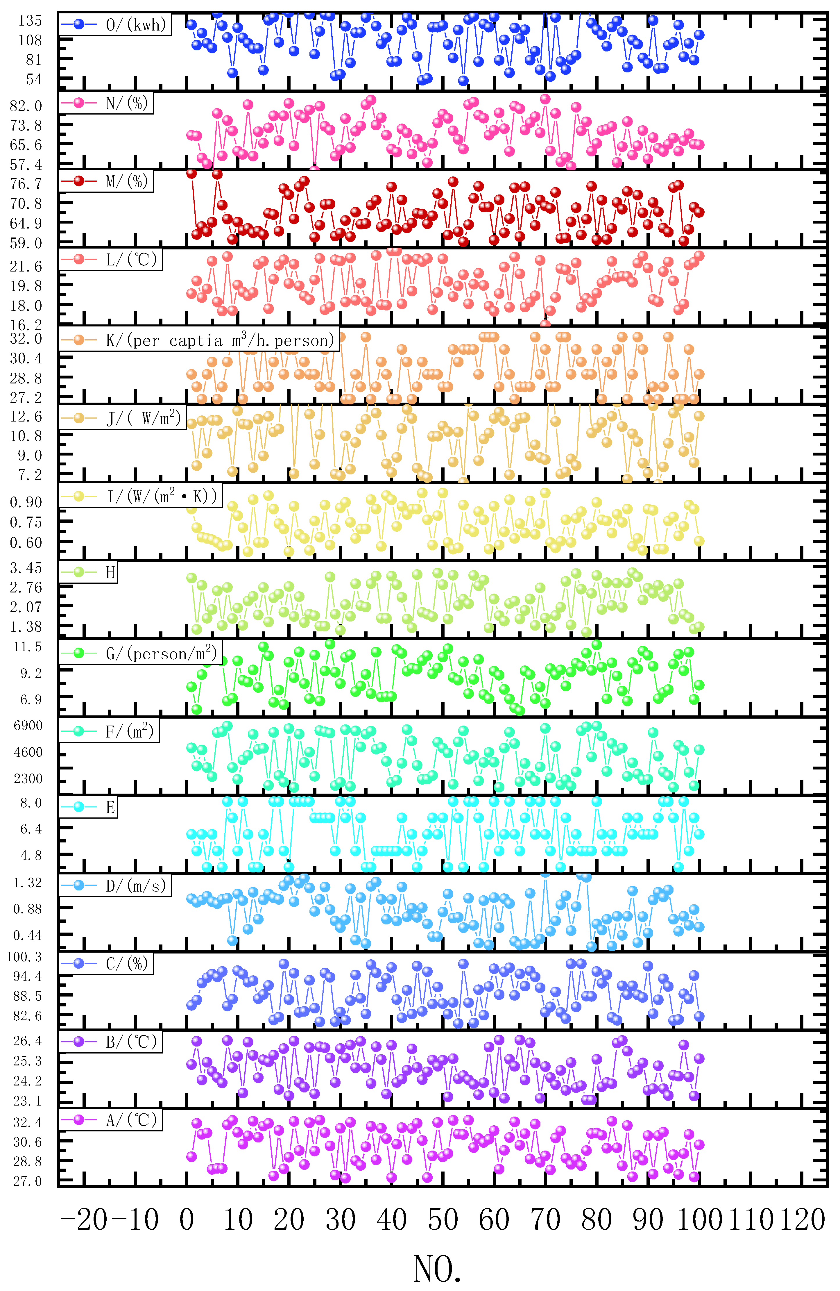
This study primarily focuses on civil public buildings as the subject of experimentation. Data encompassing energy consumption values and influencing factors were collected from 100 civil public buildings in Wuhan during April 2022 under various energy consumption conditions. In 2022, Wuhan city recorded a permanent population of 13.739 million inhabitants, located between 113°41′–115°05′ longitude east and 29°58′–31°22′ latitude north. The city resides within the middle and lower reaches of the Yangtze River Plain, eastern Jianghan Plain, with an area of 8494 square kilometers. The 15 input variable indices include outdoor temperature, indoor temperature, relative humidity, wind speed, floor level, building area, personnel density, building aspect ratio, roof heat transfer coefficient, lighting power density, per capita fresh air volume, supply air temperature, fan efficiency, pump efficiency, with energy dissipation serving as the output scalar index. To facilitate subsequent analysis, these 15 variables are represented by alphabetic letters A through O for each variable level. The original data samples are shown in Figure 1.
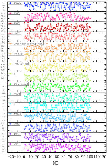
Figure 1.
Source dataset.
In addition, the descriptive statistics of 15 variables are given, such as minimum, maximum, mean, and standard deviation. The S-W normality test was performed on each variable, see Table 1. Median: this is the value in the middle after sorting all observations. It is a measure of the central trend of the data and has good robustness to outliers. Average: this is the average of all observations. It is also a measure of the central trend of the data, but may be affected by outliers. Standard deviation: this is a measure of the average degree to which the observed value deviates from the average. The larger the standard deviation, the more dispersed the distribution of data. Skewness: this is a measure of the degree of asymmetry of data distribution. A negative skewness indicates that the data are skewed to the right, that is, there is a long left tail; a positive skewness indicates that the data are skewed to the left, that is, there is a long right tail. Kurtosis: this is a measure of the degree of sharp or flat data distribution. A negative kurtosis indicates that the distribution of the data is flatter than the normal distribution; a positive kurtosis indicates that the distribution of the data is sharper than the normal distribution. S-W test: this is the result of the Shapiro–Wilk test, which is used to test whether the data conform to a normal distribution. The first number in parentheses is the test statistic, and the second number is the p-value. The results showed that using the S-W test, the significant p value was 0.007 ***, the level was significant, the null hypothesis was rejected, and the data did not meet the normal distribution.

Table 1.
Descriptive statistics by variable.
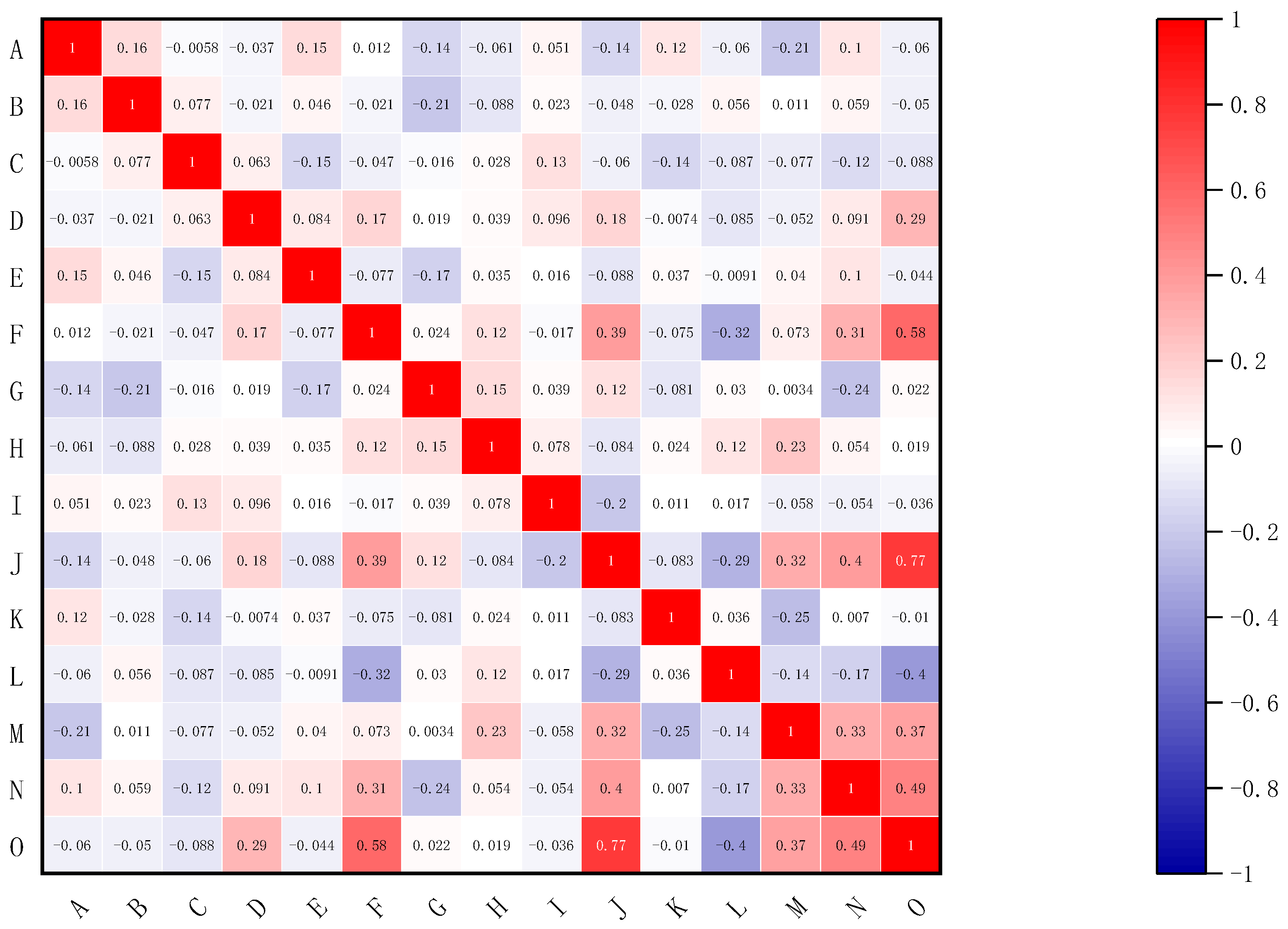
Preventing data redundancy, which refers to the unnecessary repetition of data, is crucial in modeling. One method to achieve this is by calculating the correlation coefficient between variables in the dataset. This technique identifies potential redundant characteristic variables and helps understand the correlation between different variables. For datasets not conforming to the normal distribution, as in this case, correlation analysis can be conducted using non-parametric tests or rank-based methods. These techniques are optimal because they do not make assumptions about the population’s distribution, as shown in Figure 2.
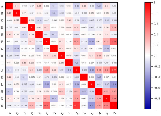
Figure 2.
Correlation matrix heat map of variables.
The correlation coefficient ranges from −1 to 1. A coefficient of 0 indicates no relationship between the two variables. In contrast, a coefficient of 1 signifies a completely positive correlation between two variables, where an increase in one variable corresponds to an increase in the other. On the other hand, a coefficient of −1 suggests a completely negative correlation, meaning that the increase of one variable corresponds to the decrease of another variable. Upon examining the correlation between the input and output variables, it is apparent that there is a significant correlation between certain variables. The heat map of the variable correlation matrix reveals a high correlation between F, J, N, and O variables, with values ranging from 0.49 to a maximum of 0.77. The remaining variables show a lower correlation with the O variable. This analysis plays an essential role in ensuring the prediction accuracy of the model.
3.2. Dimensionality Reduction with PCA
Principal component analysis (PCA) is a multivariate statistical method that uses the idea of dimension reduction to recombine the original indicators with a certain correlation into a new set of comprehensive indicators without overlapping information under the premise of less information loss. At the same time, according to certain principles and actual needs, several comprehensive indicators are recombined to reflect the amount of information carried by most of the original indicators. The calculation steps of principal component analysis are as follows:
Step 1. Establish a matrix, m is the number of samples, n is the number of indicators for each sample.
Step 2. The original data are standardized to generate a standardized matrix. The standardized calculation formula is as follows:
where is the arithmetic mean of , and is the standard deviation of ,, .
Step 3. KMO and Bartlett sphericity tests were performed. If the KMO statistic value is greater than 0.5, it can be seen that the correlation between variables is not much different, indicating that the data are suitable for factor analysis; the result of Bartlett’s spherical test is less than 0.05, the spherical hypothesis is rejected, and there is a correlation between the original variables, indicating that the data are suitable for factor analysis.
Step 4. The covariance matrix is established according to the standardized matrix. The covariance calculation formula is as follows:
where , .
The covariance matrix is composed of the covariance of two columns of variables in the standardized matrix, so is the correlation coefficient between column variables and , that is, the covariance matrix is the correlation coefficient matrix.
Step 5. Calculate the non-negative eigenvalue of the covariance matrix . The characteristic equation of covariance matrix is as follows:
Step 6. The cumulative contribution rate of the first q principal component is calculated from the calculated p non-negative eigenvalue. The calculation formula is as follows:
Step 7. According to the cumulative contribution rate of principal components, the number of principal components is selected and new variable indicators are generated. When the cumulative contribution rate of the current principal component exceeds 85%, it can be considered that these principal components can contain most of the information carried by the overall. After generating the new variable index, it is used to represent the original variable index:
Among them, is the original variable index, is the new variable index, and are not related to each other, and satisfies. Thus, the data dimension reduction is completed, and the number of variables is reduced under the premise of less information loss.
As described above, the construction of a building energy consumption model, which leverages various optimization algorithms to optimize the relevance vector machine, involves selecting 15 variables as the key influencers of energy consumption. This collection of multiple factors composes the high-dimensional data, thereby increasing the complexity of model training. However, leveraging the core concept of principal component analysis (PCA), these original high-dimensional data can be more effectively mapped to a new low-dimensional space, while retaining as much of the original data information as possible. Although numerous factors impact energy dissipation, the model’s complexity is reduced by selecting the most critical principal component to lessen the number of features. The specific process of analysis is detailed in the following steps:
Step a: First, KMO and Bartlett tests are performed to determine whether principal component analysis can be performed. KMO test and Bartlett test can help to determine whether the data are suitable for factor analysis, and can help to select the best number of factors. Therefore, before factor analysis, KMO test and Bartlett test can improve the reliability and accuracy of factor analysis. The test results are shown in Table 2.

Table 2.
KMO test and Bartlett test.
The KMO test results showed that the KMO value was 0.455. At the same time, the results of the Bartlett spherical test showed that the significant p value was 0.000 ***, which was significant at the level, rejecting the original hypothesis. There was a correlation between the variables, and the principal component analysis was practical.
Step b: The principal component analysis (PCA) is a statistical procedure that transforms a number of possibly correlated variables into a smaller number of uncorrelated variables called principal components. It is essential when performing PCA to determine the number of principal components that should be retained to keep sufficient information and minimize dimensions. The variance interpretation table plays a key role in this determination. It is used to understand the degree to which each principal component contributes to the variance of the original variable, also known as the contribution rate. In general, only the principal components whose cumulative contribution rate reaches a certain threshold are retained. This threshold typically lies between 60% and 85%. The Scree plot, often referred to as the gravel map, aids in this process. It helps determine the number of principal components to retain, based on the size of their eigenvalues and the rate at which these eigenvalues decline. Here, the term eigenvalue, also referred to as the characteristic root within PCA or factor analysis, denotes the proportion of the total variance attributable to each principal component or factor. Principal components or factors with eigenvalues exceeding 1 are typically deemed significant as they explain greater variance than the average variance of an individual variable. The combination of these two methods helps to decide the final number of principal components that should be retained to achieve effective dimensionality reduction, as shown in Table 3. The variance explained ratio represents the proportion of the total variance that each principal component or factor accounts for. This overall methodology ensures that the contribution rate of the principal components is high enough to provide meaningful insights.

Table 3.
All factor variance explanation table.
When the principal component is 7, the characteristic root explained by the total variance is higher than 1, and the cumulative variance explanation rate is 66.106%. When the principal component is 8, the characteristic root of the total variance explanation is much lower than 1. This paper selects 7 principal component factors for data dimensionality reduction.
Step c: By analyzing the principal component load coefficient and the heat map, the importance of the hidden variables in each principal component can be analyzed, see Table 4. The value of the factor loading coefficient is generally between −1 and 1. The larger the absolute value of the value, the stronger the correlation between the original variable and the corresponding principal component or factor. The negative load indicates that the relationship between the original variable and the principal component or factor is negatively correlated, while the positive load indicates a positive correlation.

Table 4.
Factor load coefficient table.
Step d: Based on the principal component loading diagram, the multi-principal components are reduced to double principal components or three principal components, and the spatial distribution of the principal components is presented by quadrant diagram. In this paper, 7 principal components are reduced for the original sample dataset.
Step e: By analyzing the component matrix, the principal component formula and weight are obtained, see Table 5.

Table 5.
Composition matrix table.
Step f: Through principal component analysis, while reducing the dimension of variables, it also ensures that the amount of information carried by the original sample data is less lost. The comprehensive score after dimensionality reduction by principal component analysis is shown in Table 6.

Table 6.
Principal component analysis dimensionality reduction data.
3.3. Model Training
Within the realm of machine learning, model parameters are derived through an adaptive learning process rather than being manually set. Typical examples of this in neural network modeling include coefficients in linear regression and weights in neural networks. In contrast, hyperparameters are certain variables required in the mathematical modeling process that are not learned from the data during training but are set prior to the commencement of the learning process. The values of these variables cannot be obtained through estimation and typically, the optimal values of hyperparameters must be determined based on experience or through repeated experimentation. Crucially, the selection of appropriate parameters and hyperparameters significantly impacts both the performance of the model and the quality of the predictions it generates. As parameters and hyperparameters interact, it is necessary to account for their integrated effects in the learning and optimization process.
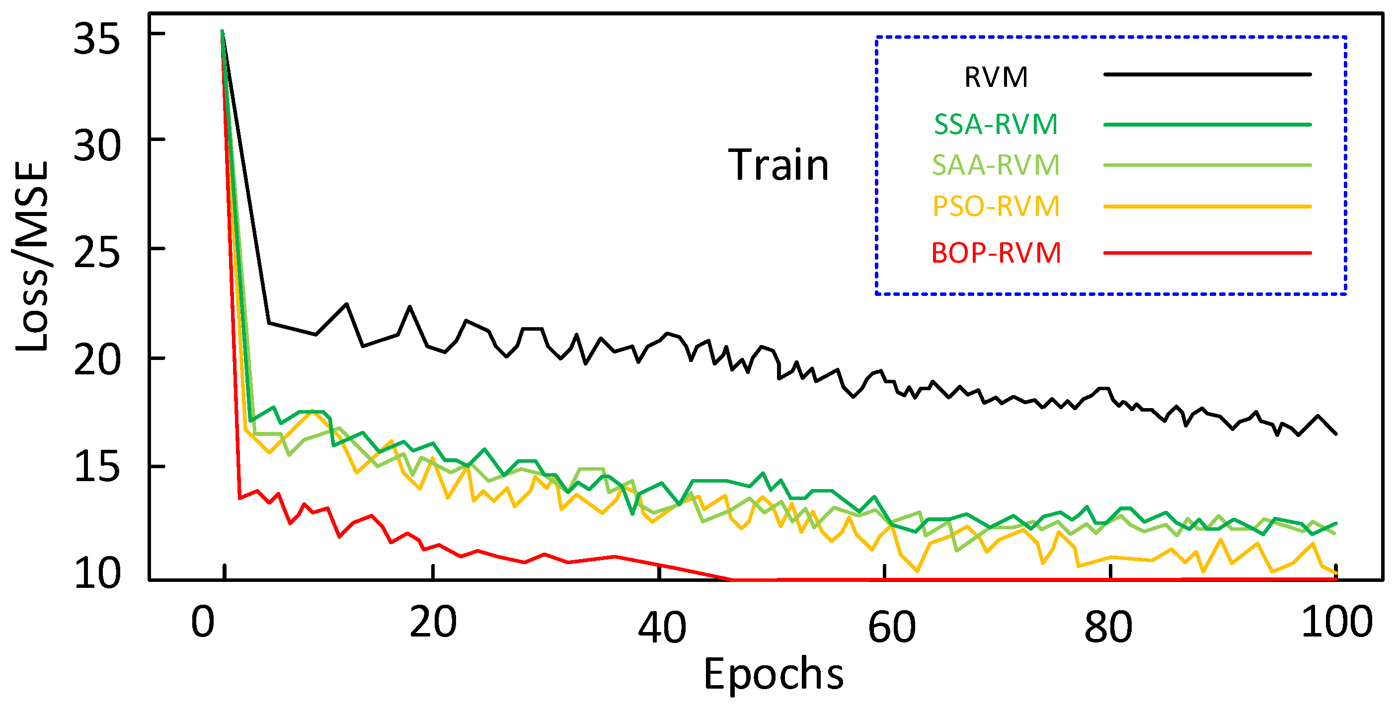
A demonstration of how these factors come into play can be seen in Table 7, which presents the values of model parameters after optimization using various algorithms discussed in Section 2. Turning our attention to Figure 3, we find the Mean Squared Error (MSE) convergence curves for the Relevance Vector Machine (RVM) model and various optimized models. The BOP-RVM model exhibits a superior convergence speed, and optimized models outperform the traditional RVM in terms of convergence speeds. Among these optimized models, however, it is notable that the use of the BOP algorithm significantly enhances both the precision of optimization and the speed of convergence.

Table 7.
The model parameters and optimization parameters.
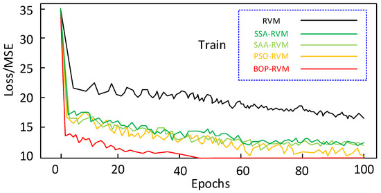
Figure 3.
MSE convergence curve.
3.4. Model Training Results
Following the dimension reduction process detailed in Section 3.2, the data were randomly organized. The first 90 data groups were selected as the training set, with the remaining 10 groups forming the test set. Using various optimization models, a building energy consumption prediction model was constructed to optimize the relevance vector machine. An analysis was performed on the characteristics of the predicted and actual values of each model. Additionally, each model’s capability to predict building energy dissipation was examined and quantified. As a result, the selection of the optimal prediction model has been achieved.
Upon completion of dimensionality reduction, 90 sets of training data were fed into the RVM model, SSA-RVM model, SAA-RVM model, PSO-RVM model, and BOP-RVM model for training. The optimal parameters obtained from Section 3.3 were individually introduced into each model. Once the training was complete, the 10 test datasets were individually introduced into each of the aforementioned models for validation. By comparing the validation results with the energy consumption values in the original data, the optimal model was determined. The construction process of the building energy dissipation prediction model based on machine learning is shown in Figure 4.
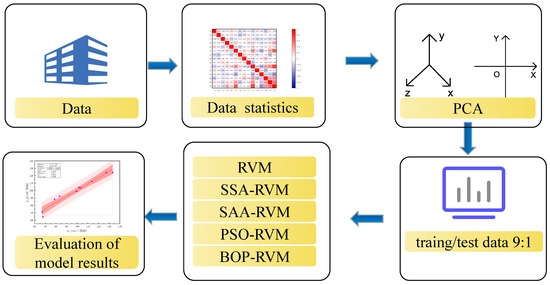
Figure 4.
Energy dissipation prediction model construction process.
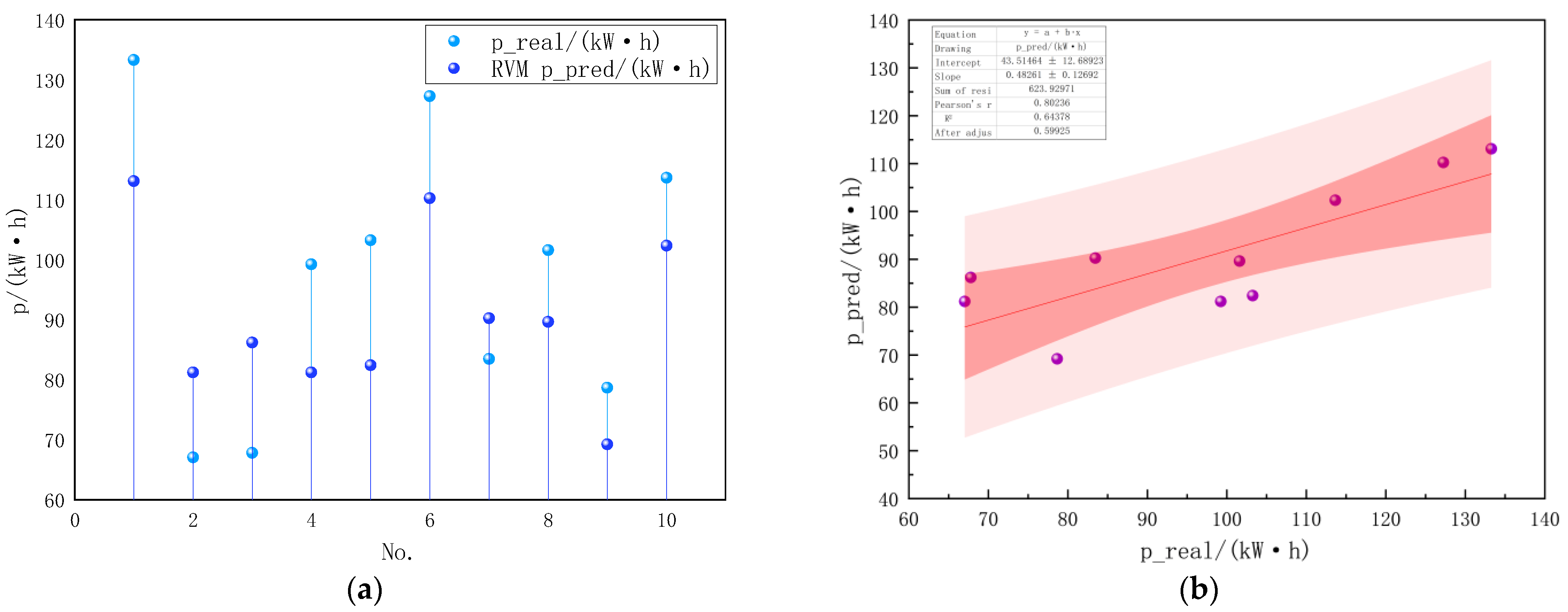
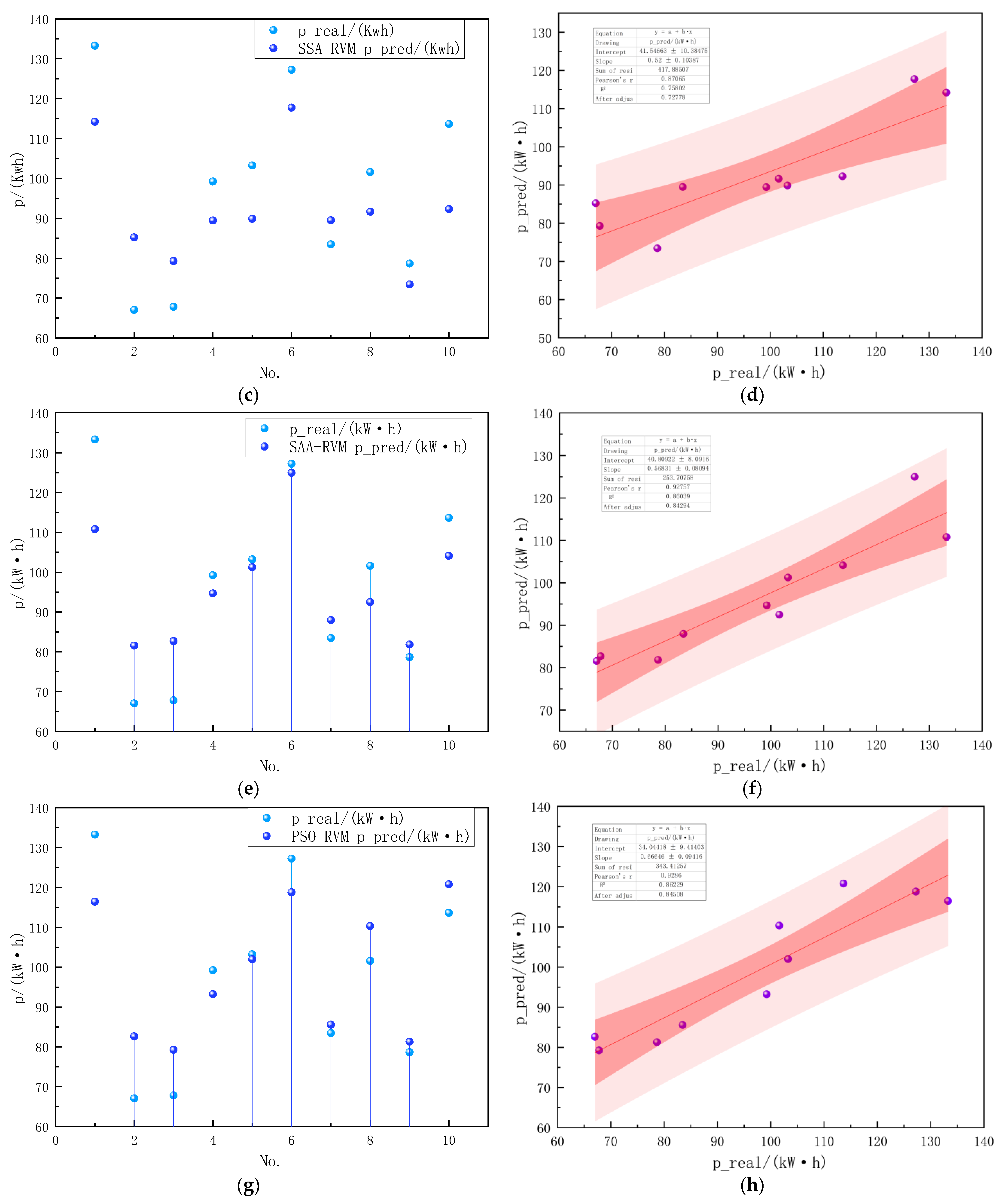
For the building energy dissipation prediction model, RVM model, SSA-RVM model, SAA-RVM model, PSO-RVM model, and BOP-RVM model are used to predict, respectively. The predicted results are shown in Figure 5, which is the scatter diagram of the predicted value and the real value obtained by the four optimization models, and the regression analysis.

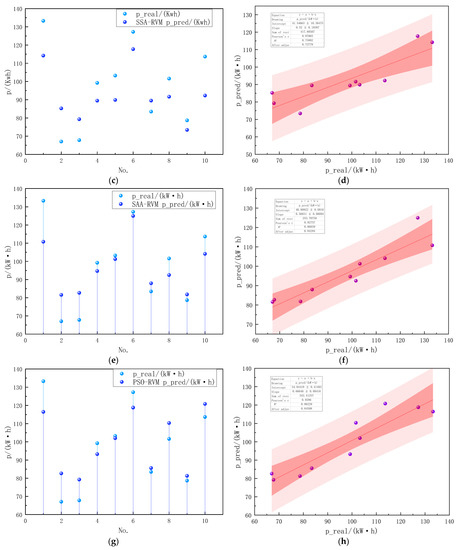
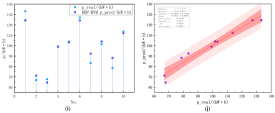
Figure 5.
Simulation results of each model. (a) The scatter of the RVM predicted value and true value. (b) RVM predicted value and true value regression. (c) The scatter of SSA-RVM predicted value and true value. (d) SSA-RVM predicted value and true value regression. (e) The scatter of SAA-RVM predicted value and true value. (f) SAA-RVM predicted value and true value regression. (g) The scatter of PSO-RVM predicted value and true value. (h) PSO-RVM predicted value and true value regression. (i) The scatter of BOP-RVM predicted value and true value. (j) BOP-RVM predicted value and true value regression.
In Figure 5b, the RVM model predicts the R2 (0.6438) between the predicted value and the true value, and the fitting regression equation is (ppred = 0.4826 preal + 43.5146); the model prediction accuracy is low. From Figure 5a, we can see that the most obvious relative error values of the RVM model are samples 1 and 5, and the calculated maximum error is 20.83.
In Figure 5c, after the SSA model parameter optimization, the error between the predicted value and the true value of sample 5 has been significantly reduced. The error of sample 5 is reduced from 20.83 kW·h to 13.38 kW·h, and the minimum error is only 5.25 kW·h. Although the relative error of samples 2 and 10 is greater than that of RVM model, the overall prediction result of SSA-RVM model is closer to the real value than that of RVM model. In Figure 5d, the R2 (0.758) between the predicted value and the real value is obtained by the SSA-RVM model prediction model; the fitting regression equation is (ppred = 0.52 preal + 41.5466).
In Figure 5e, after SAA model parameter optimization, the error between the predicted value and the true value of the sample 4–6 has been significantly reduced. The relative error of the model is below 10 kW·h, and the error of the sample 1 is 22.49 kW·h. The overall prediction results of the SSA-RVM model are closer to the true value than the RVM model. In Figure 5f, the R2 (0.8604) between the predicted value and the real value obtained by the SAA-RVM model prediction model, the fitting regression equation is (ppred = 0.5683 preal + 40.8092).
In Figure 5g, after the PSO model parameters are optimized, the overall prediction results of the PSO-RVM model are relatively stable. In Figure 5h, the R2 (0.8623) between the predicted value and the real value is obtained by the PSO-RVM model prediction model; the fitting regression equation is (ppred = 0.6665 preal + 34.0442).
In Figure 5i, after the BOP model parameters are optimized, the error between the predicted value and the true value of the samples 1–10 is significantly reduced. The relative error of the model is below 10 kW·h, and the error of the sample 8 is 9.65 kW·h. The overall prediction result of the BOP-RVM model is closer to the true value than other optimization models. In Figure 5j, the R2 (0.9528) is between the predicted value and the real value obtained by the BOP-RVM model prediction model; the fitting regression equation is (ppred = 0.8444 preal + 16.0966).
With the construction of the model for the prediction of building energy dissipation, when we get the model’s predicted value, how to judge the deviation between the expected value and the measured value is also essential to research. Therefore, when evaluating the predictive value of the machine learning model, various evaluation indicators are selected, which can comprehensively reflect the performance of the constructed model. Root mean square error (RMSE), coefficient of determination (R2), correlation coefficient (r), and Scatter Index (SI) were used as indicators to measure the prediction effect of the model. RMSE is the most commonly used to measure the prediction effect of the regression model, which can better reflect the deviation between the predicted value and the actual value. For RMSE [0, ∞), the smaller the value, the better the prediction effect. R2 represents the extent to which the regression model can explain the change of the target variable and reflect the model’s goodness of fit. For R2 (−∞, 1], the larger the R2, the better the fitting. If it is negative, the prediction effect of the regression model is not as good as the average value of the target variable. r represents the degree of linear correlation between the predicted value and the real value, r [−1, 1]; the more significant the absolute value, the more substantial the correlation, and the higher the degree of model matching.
where ppred is the predicted energy dissipation prediction value, preal is the observed energy dissipation, is the average predicted energy dissipation, and is the average observed energy dissipation, is the standard deviation of the prediction error, is the average value of the true value. The evaluation results of each model are shown in Table 8. Comparing the prediction accuracy of the four optimization models and the RVM model, it is found that the optimization model can better improve the prediction accuracy of building energy dissipation. The BOP-RVM model has the highest model prediction accuracy and can better improve the accuracy between the predicted value and the actual value.

Table 8.
Model evaluation.
Based on Table 7 results, it was observed that the RVM model performed worst among all indicators. The model’s coefficient of determination is only 0.6438, indicating that the model has a limited ability to interpret the observed data. The linear correlation value is 0.8024, which shows that the linear correlation between the model and the observation data is weak. At the same time, the root mean square error reaches 23.1517, which means that the model’s prediction accuracy is relatively low. Therefore, from the perspective of all-around performance, the fitting effect and prediction ability of the RVM model could be better.
In comparison to the standalone RVM model, the other four models—namely BOP-RVM, SAA-RVM, PSO-RVM, and SSA-RVM—showcase superior performance. Among them, the BOP-RVM model stands out with impressive scores in key metrics: determination coefficient (0.9528), linear correlation value (0.9761), and root mean square error (5.3894). These statistics reveal that the BOP-RVM model not only explains the changes in observation data exceptionally well but also boasts high prediction accuracy.
Following closely are the SAA-RVM and PSO-RVM models, demonstrating robust overall performance. The SAA-RVM model achieves a determination coefficient of 0.9276, a linear correlation value of 0.8604, and a root mean square error of 9.6136. Meanwhile, the PSO-RVM model obtains a determination coefficient of 0.8623, a linear correlation value of 0.9286, and a root mean square error of 9.6395. Both models manage to provide compelling explanations for the observed data and maintain high prediction accuracy.
The SSA-RVM model, however, ranks in the middle of the pack in terms of overall performance, with a determination coefficient of 0.7580, a linear correlation value of 0.8707, and a root mean square error of 13.9313. Despite its reasonable fitting effects and prediction accuracy, it still falls short when compared to other models.
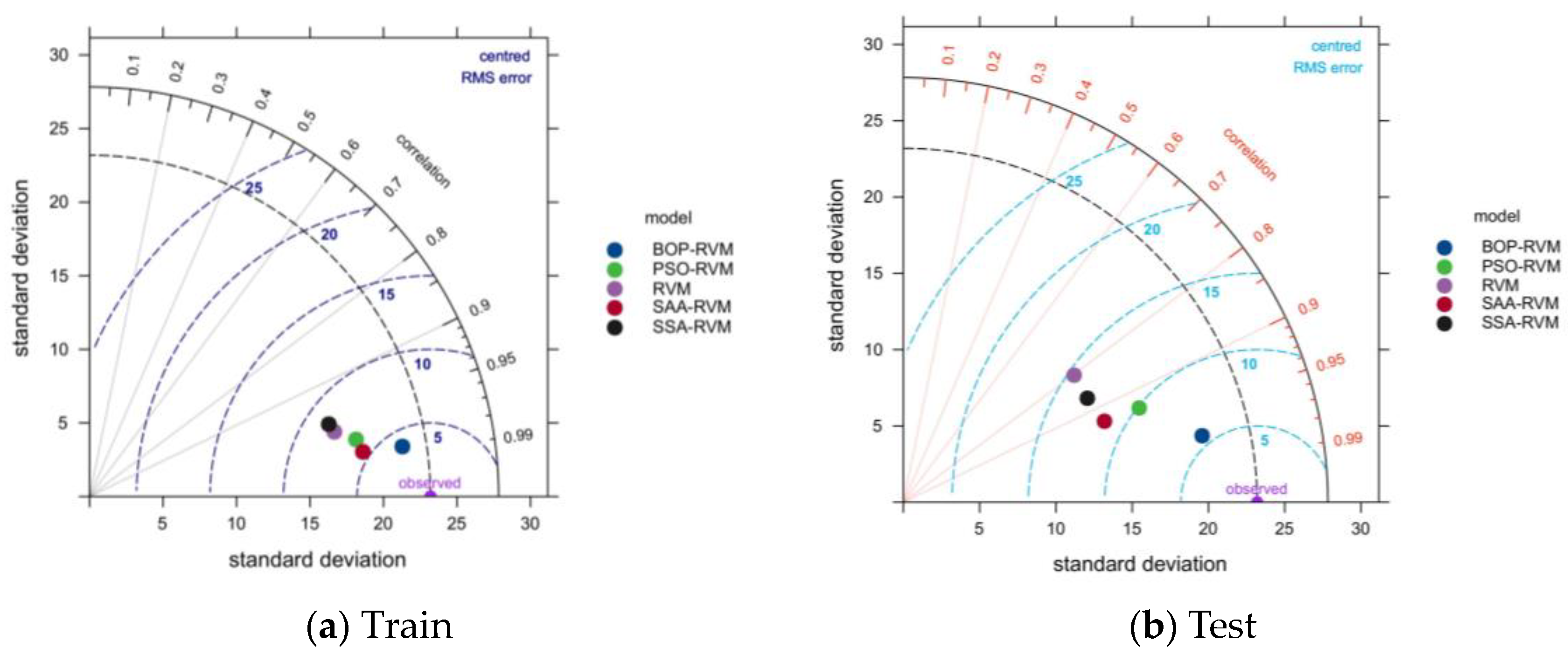
To provide a more comprehensive comparison, we introduced the Taylor diagram as a tool to evaluate the prediction accuracy of each model (refer to Figure 6). The diagram indicates that the BOP-RVM model sits closest to the observed point, signifying its superior prediction accuracy among the five models.
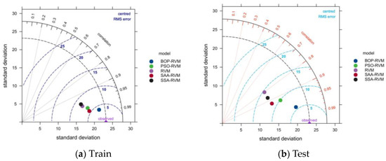
Figure 6.
Taylor evaluation.
Focusing on the performance metrics within the training set, all models exhibit a high level of predictive accuracy. In fact, the standard deviation, root mean square error, and correlation coefficients closely approximate the observed distances. However, when the models are applied to the test set, which consists of different data than the training set, discrepancies emerge. In this scenario, the optimized RVM models, particularly the BOP-RVM, outshine the standalone RVM model across all three evaluation metrics. This observation underscores the BOP-RVM model’s superior performance in both training and test settings, thus affirming its potential for future applications.
In summary, by comparing and analyzing the performance indicators of each model, it is found that the BOP-RVM model performs best in comprehensive performance, with a high determination coefficient, linear correlation value, and low root mean square error. Secondly, SAA-RVM and PSO-RVM models perform well in all-around performance. The SSA-RVM model ranks in the middle, while the RVM model performs worst among all indicators.
4. Conclusions
The goal of this study is to establish a building energy consumption prediction model, utilizing machine learning methods, to enhance our understanding and predictive accuracy of energy use in civil public buildings. Various machine learning-based models were scrutinized in this investigation, with the BOP-RVM model displaying superior comprehensive performance. It demonstrated a higher determination coefficient, a significant linear correlation value, and a lower root mean square error, illustrating its ability to effectively interpret observed data changes and provide highly accurate predictions. The SAA-RVM and PSO-RVM models also exhibited commendable performances, while the SSA-RVM and RVM models trailed slightly in overall performance. An in-depth correlation analysis of 14 factors affecting civil building energy dissipation revealed three prominent contributors: building area, personnel density, and air supply temperature. To mitigate energy dissipation in Wuhan’s local civil buildings, these three indicators should be considered when formulating energy management and optimization strategies during the preliminary architectural design phase.
For existing structures, we recommend prioritizing the BOP-RVM model for predicting and analyzing building energy consumption. This machine learning-based approach can enhance the understanding and prediction of building energy consumption, providing a more scientifically sound and rational basis for building energy management. By doing so, it can facilitate energy waste reduction, efficiency improvement, and positively influence sustainable building development.
Future studies should persist in exploring and optimizing these machine learning models. Including more relevant factors, such as the specifics of building design and usage, into the model can further augment prediction accuracy and application value.
Author Contributions
Conceptualization, H.W. and Z.Z.; methodology, H.W.; software, N.G.; validation, H.W., W.W., Z.Z. and N.G.; formal analysis, Z.Z.; investigation, W.W.; resources, H.W.; data curation, H.W.; writing—original draft preparation, H.W.; writing—review and editing, H.W.; visualization, H.W.; supervision, H.W.; project administration, H.W.; funding acquisition, Z.Z. All authors have read and agreed to the published version of the manuscript.
Funding
This research received no external funding.
Data Availability Statement
All data generated or analyzed during the study are available from the corresponding author by request.
Conflicts of Interest
The authors declare no conflict of interest.
References
- Wu, J.; Wei, Y.; Zhang, X. Prediction of Occupancy Level and Energy Consumption in Office Building Using Blind System Identification and Neural Networks. Appl. Energy 2019, 240, 276–294. [Google Scholar]
- Qiang, G.; Zhe, T.; Yan, D.; Neng, Z. An Improved Office Building Cooling Load Prediction Model Based on Multivariable Linear Regression. Energy Build. 2015, 107, 445–455. [Google Scholar] [CrossRef]
- Cooney, E.W. Long waves in building in the british economy of the nineteenth century. Econ. Hist. Rev. 1960, 13, 257–269. [Google Scholar] [CrossRef]
- Zhao, H.X.; Magoulès, F. A review on the prediction of building energy consumption. Renew. Sustain. Energy Rev. 2012, 16, 3586. [Google Scholar] [CrossRef]
- Amasyali, K.; El-Gohary, N.M. A review of data-driven building energy consumption prediction studies. Renew. Sustain. Energy Rev. 2018, 81 Pt 1, 1192–1205. [Google Scholar] [CrossRef]
- Wang, Z.; Srinivasan, R.S. A review of artificial intelligence based building energy use prediction: Contrasting the capabilities of single and ensemble prediction models. Renew. Sustain. Energy Rev. 2016, 75, 796. [Google Scholar] [CrossRef]
- Foucquier, A.; Robert, S.; Suard, F.; Stephan, L.; Jay, A. State of the art in building modelling and energy performances prediction: A review. Renew. Sustain. Energy Rev. 2013, 23, 272. [Google Scholar] [CrossRef]
- Lei, L.; Chen, W.; Wu, B.; Chen, C.; Liu, W. A building energy consumption prediction model based on rough set theory and deep learning algorithms. Energy Build. 2021, 240, 110886. [Google Scholar] [CrossRef]
- Fan, C.; Xiao, F.; Zhao, Y. A short-term building cooling load prediction method using deep learning algorithms. Appl. Energy 2017, 195, 222–233. [Google Scholar] [CrossRef]
- Guo, J.J.; Wu, J.Y.; Wang, R.Z. A new approach to energy consumption prediction of domestic heat pump water heater based on grey system theory. Energy Build. 2011, 43, 1273–1279. [Google Scholar] [CrossRef]
- Zhang, C.; Zhao, Y.; Zhang, X.; Fan, C.; Li, T. An Improved Cooling Load Prediction Method for Buildings with the Estimation of Prediction Intervals. Procedia Eng. 2017, 205, 2422–2428. [Google Scholar] [CrossRef]
- Fan, C.; Liao, Y.; Ding, Y. Development of a cooling load prediction model for air-conditioning system control of office buildings. Int. J. Low Carbon Technol. 2019, 14, 70–75. [Google Scholar] [CrossRef]
- Ekici, B.B.; Aksoy, U.T. Prediction of building energy consumption by using artificial neural networks. Adv. Eng. Softw. 2009, 40, 356–362. [Google Scholar] [CrossRef]
- Dahl, C.A. Energy Efficiency: Building a Clean, Secure Economy. Energy J. 2017, 38, 232. [Google Scholar]
- Braun, J.; Chaturvedi, N. An Inverse Gray-Box Model for Transient Building Load Prediction. HVACR Res. 2002, 8, 73–99. [Google Scholar] [CrossRef]
- Chen, S.; Zhou, X.; Zhou, G.; Fan, C.; Ding, P.; Chen, Q. An online physical-based multiple linear regression model for building’s hourly cooling load prediction. Energy Build. 2022, 254, 111574. [Google Scholar] [CrossRef]
- Sarkhani, B.R.; Esmaeili, F.M.; Javadi, A. Predicting resilient modulus of flexible pavement foundation using extreme gradient boosting based optimised models. Int. J. Pavement Eng. 2022, 2022, 1–20. [Google Scholar] [CrossRef]
- Kwok, S.S.K.; Lee, E.W.M. A study of the importance of occupancy to building cooling load in prediction by intelligent approach. Energy Convers. Manag. 2011, 52, 2555–2564. [Google Scholar] [CrossRef]
- Mahzad, E.F.; Reza, S.B. Ensemble deep learning-based models to predict the resilient modulus of modified base materials subjected to wet-dry cycles. Geomech. Eng. 2023, 32, 583–600. [Google Scholar]
- Fumo, N. A review on the basics of building energy estimation. Renew. Sustain. Energy Rev. 2014, 31, 53–60. [Google Scholar] [CrossRef]
- Wang, Z.; Srinivasan, R.S. A review of artificial intelligence based building energy prediction with a focus on ensemble prediction models. In Proceedings of the 2015 Winter Simulation Conference (WSC), Huntington Beach, CA, USA, 6–9 December 2015. [Google Scholar]
- Jain, R.K.; Smith, K.M.; Culligan, P.J.; Taylor, J.E. Forecasting energy consumption of multi-family residential buildings using support vector regression: Investigating the impact of temporal and spatial monitoring granularity on performance accuracy. Appl. Energy 2014, 123, 168–178. [Google Scholar] [CrossRef]
- Karatasou, S.; Santamouris, M.; Geros, V. Modeling and predicting building’s energy use with artificial neural networks: Methods and results. Energy Build. 2006, 38, 949–958. [Google Scholar] [CrossRef]
- Tserng, H.P.; Chou, C.M.; Chang, Y.T. The Key Strategies to Implement Circular Economy in Building Projects Case Study of Taiwan. Sustainability 2021, 13, 754. [Google Scholar] [CrossRef]
- Niu, Y.; Cheng, H.; Wu, S.; Sun, J.; Wang, J. Rheological properties of cemented paste backfill and the construction of a prediction model. Case Stud. Constr. Mater. 2022, 16, e01140. [Google Scholar] [CrossRef]
- Zhang, Z.; Wang, H.; Gao, N. Simulation and parameter prediction model of rheological properties of fiber reinforced concrete. Case Stud. Constr. Mater. 2023, 18, e01963. [Google Scholar] [CrossRef]
Disclaimer/Publisher’s Note: The statements, opinions and data contained in all publications are solely those of the individual author(s) and contributor(s) and not of MDPI and/or the editor(s). MDPI and/or the editor(s) disclaim responsibility for any injury to people or property resulting from any ideas, methods, instructions or products referred to in the content. |
© 2023 by the authors. Licensee MDPI, Basel, Switzerland. This article is an open access article distributed under the terms and conditions of the Creative Commons Attribution (CC BY) license (https://creativecommons.org/licenses/by/4.0/).

