A Review of Building Carbon Emission Accounting and Prediction Models

Abstract

As an industry that consumes a quarter of social energy and emits a third of greenhouse gases, the construction industry has an important responsibility to achieve carbon peaking and carbon neutrality. Based on Web of Science, Science-Direct, and CNKI, the accounting and prediction models of carbon emissions from buildings are reviewed. The carbon emission factor method, mass balance method, and actual measurement method are analyzed. The top-down and bottom-up carbon emission accounting models and their subdivision models are introduced and analyzed. Individual building carbon emission assessments generally adopt a bottom-up physical model, while urban carbon emission assessments generally adopt a top-down economic input-output model. Most of the current studies on building carbon emission prediction models follow the path of “exploring influencing factors then putting forward prediction models based on influencing factors”. The studies on driving factors of carbon emission mainly use the Stochastic Impacts by Regression on Population, Affluence, and Technology (STIRPAT) model, the Logarithmic Mean Divisia Index (LMDI) model, the grey correlation degree model, and other models. The prediction model is realized by the regression model, the system dynamics model, and other mathematical models, as well as the Artificial Neural Network (ANN) model, the Support Vector Machine (SVM) model, and other machine learning models. At present, the research on carbon emission models of individual buildings mainly focuses on the prediction of operational energy consumption, and the research models for the other stages should become a focus in future research.

1. Introduction

Over the past 100 years, the concentration of carbon dioxide in the atmosphere has increased significantly and continues to increase at a rate of 2 ppm/year [1]. With the annual increase in atmospheric greenhouse gas emissions, global warming has become the most serious environmental problem mankind has ever faced. Tests show that from 1880 to 2012, the average global temperature rose by 0.85 owing to the influence of the greenhouse effect [2,3], which will continue to have a significant impact on natural ecology and social economy in the future [4,5].

To avoid disastrous consequences, the Paris Agreement committed the world to keeping the global average temperature rise below 2 degrees Celsius above pre-industrial levels within this century, and to make efforts to limit the rise to 1.5 degrees Celsius [6,7,8,9]. Global greenhouse gas emissions will peak as soon as possible and reach net zero emissions in the second half of this century. The construction industry consumes about a quarter of the energy of the whole society, and contributes about a third of the carbon emissions and nearly 50% of the carbon dioxide emissions for the whole life cycle when the production, transportation and construction of building materials is considered [10,11]. Compared with other industries, the building industry has great potential to save energy per unit cost. Between 2021 and 2060, the embodied carbon emissions of China’s construction industry are expected to fall by between 20.9 billion and 45.3 billion tons of carbon dioxide, while carbon emission levels in 2060 are expected to be 49% lower than in 2020, and the emission reduction space is huge [12].

The detailed accounting of building carbon emissions is the basis of building energy saving and emission reduction. Zhang and Yan [13] proposed a process-based building life cycle assessment model to discuss the energy consumption and carbon emission trends of China’s building industry from 2000 to 2016. The study found that building scale, building structure type, and material production efficiency are three important drivers of carbon emissions. In order to simulate the carbon emissions of different economic sectors, Zhou and Li [14] proposed a Bayesian neural network model (IO-BNN) based on the economic input-output method. The authors use this model to study Guangdong’s carbon emissions, and the results show that Guangdong’s carbon emissions are expected to peak in 2025 under the optimal policy scenario.

Predicting building carbon emissions is necessary to realize building carbon neutrality. The STIRPAT model, LMDI model, regression model, grey system theory, and other models are widely used in the field of carbon emission accounting [15,16,17,18]. Wang and Hu [19] compared four machine learning-based generators using one year of measured data to achieve optimal thermal comfort management and carbon emission prediction for public buildings in large Spaces. The optimization results show that the hybrid machine learning model can reduce carbon emissions further than manual management. Yang and Wang [20] propose a combined prediction model for predicting carbon emissions. The combined model first decomposed the original data twice, then used the chameleon swarm algorithm and carnivorous plant algorithm to train kernel parameters, and finally used the model to predict carbon emissions. It was found that each index of this model is better than other comparison models.

In conclusion, there are various accounting models and prediction models for building carbon emission assessment, each with different emphases. However, there is a lack of systematic research on the above two types of models. What models are available for carbon emissions accounting and prediction? How accurate are their calculations? What is their scope of use? What are the differences between the models? Which models can play a more important role in the implementation of the national “carbon peaking and carbon neutrality” strategy? In order to answer the above questions, this paper will make a comprehensive review of building carbon emission accounting models and prediction models. The contributions of this paper are as follows: (1) The principles and application scenarios of the carbon emission factor method, measurement method, and mass balance method are discussed. (2) The differences and connections between three common building carbon emission accounting models (the process-based method, economic input-output method, and hybrid method) are analyzed. (3) The basic principles and applications of mathematical prediction models (such as the factor decomposition method, regression model, and gray system theory) and machine learning prediction models (such as the neural network and support vector machine models) are discussed. It is expected that this study will provide a reference for the reduction of carbon dioxide emissions in the construction industry and contribute to the realization of carbon peaking and carbon neutrality goals as soon as possible.

2. Methodology

The methodological design of literature reviews plays an indispensable role in scientific research. This section introduces the research scope, the search process, the search result, and the inclusion criteria of the articles by means of a systematic review.

2.1. Research Scope

According to the detailed definition of the whole life cycle of buildings given by GB/T 51366-2019 [21], the research scope of this paper is as follows: the carbon emission calculation model and the prediction model related to the production and transportation of building materials, construction and demolition, operation and other activities, including macro and micro levels.

This paper aims to answer the question: “Which building carbon emission accounting models and prediction models are available respectively, and what are their advantages and disadvantages and applicable scenarios”. This paper searched for relevant literature from recent years. The literature used in this paper was mainly identified by searching three databases: Web of Science, Science-Direct, and CNKI, while Engineering Village 2 and Google Academic were used as supplementary searches. As a search record, we used the keywords outlined below.

Keywords related to the model: building carbon emissions, life cycle, the whole life cycle assessment, top-bottom, bottom-up, economic input-output method, process-based method (PB method), hybrid method, measurement method, carbon emission factors, boundary conditions, building materials production, building materials transportation, construction, demolition, maintenance, residential buildings, public buildings, commercial buildings, educational buildings, frame structures, brick-and-concrete structures, wood structures, ISO14000 series.

Keywords related to prediction model: pre-evaluation, big data analysis, factor analysis, mathematical model, machine learning, evaluation tool, physical model, statistical model.

In addition, parts of the bibliography of the retrieved articles are also included in the scope of review, including the cited case buildings.

In order to obtain more comprehensive analysis results, the research results of the last 15 years were searched. Only papers published in peer-reviewed journals were considered. In the initial search, more than 147,000 studies related to the above keywords were obtained. The selection was divided into three rounds. In the first round, 520 relevant studies were obtained according to the title and abstract. In the second round, a total of 128 relevant papers were obtained by skimming the full text. In the third round, 45 studies that are highly relevant to the research topic were identified through intensive reading of the full text.

2.2. Criteria for Data Screening

Further screening of 520 relevant studies followed the following criteria:

• Is the object of study a single building or regional complex, rather than a single component within the building?
• Does the study explicitly use a carbon emission calculation model or prediction model?
• Did the study conduct a case study of the model used and analyze the advantages and disadvantages?

2.3. Carbon Emission Accounting Methods

In order to further summarize the 45 papers, this paper divided them into two categories: the carbon emission accounting model, and the prediction model. In the accounting model, we focus on the characteristics of each model and its scope of application, while in the prediction model, we focus on its interpretation and application.

3. Carbon Emission Accounting Model

3.1. Carbon Emission Accounting Methods

Carbon emission accounting provides reliable data support and a solid basic guarantee for promoting the green and low-carbon transformation of the economy and society. At present, there are three carbon emission accounting methods widely used in the world: the carbon emission factor method, the mass balance method, and the measurement method [22]. These three methods are suitable for different industries and different conditions of use.

In 1996, the IPCC compiled and published the first edition of the Guidelines for National Greenhouse Gas Emission Inventories. This put forward the carbon emission factor method, which is the most widely-used method of carbon emission accounting at present [23]. The idea of this method is to find activity data (A) and the emission factor (EF) for each emission source according to the carbon emission inventory list, and take the product of the two as the estimated carbon emission (E), that is:

$$E=A\times EF$$

(1)

where $E$ is greenhouse gas emission (such as CO₂, CH₄, et al.); $A$ is activity data (specific amount of use directly related to carbon emissions by a single emission source); $EF$ is the carbon emission factor, which is the amount of greenhouse gases released per unit of use of an emission source. Data sources can be found in various carbon emission factor databases, such as the Emission Factor Database (EFDB) of the International Panel on Climate Change (IPCC), and the China Products Carbon Footprint Factors Database (CPCD) of China.

The advantage of using the carbon emission factor method to calculate carbon emissions is that the process is simple, easy to understand, and has strong operability. This method can be applied to the calculation of carbon emissions at the micro or macro scales. More importantly, various countries and industries have created rich carbon emission factor databases for inquiry [24]. However, its shortcomings are also obvious: the carbon emission factors in these databases are highly regional and highly uncertain.

The basic principle of the mass balance method is the law of conservation of mass, that is, the carbon content of the input material is equal to the sum of the carbon content of all the output material [25], that is:

$$E=\left[{\displaystyle \sum \left(M_{in}\times C_{in}\right)-{\displaystyle \sum \left(M_{\mathit{out}}\times C_{\mathit{out}}\right)}}\right]\times \frac{44}{12}\times GWP$$

(2)

where $M_{in}$ is the input material quantity; $C_{in}$ is the carbon content of the input material; $M_{out}$ is the output material quantity; $C_{out}$ is the carbon content of the output material; $\frac{44}{12}$ is the conversion coefficient of carbon element to carbon dioxide; GWP is the global warming potential. The advantage of this method lies in the systematic and detailed study of the carbon emissions in the production process, which is more scientific and rigorous, but the disadvantage is that it requires a comprehensive understanding of the production process.

As the name implies, the measurement method calculates carbon emissions by using special instruments to measure the velocity, discharge and concentration of the emitted gas [26]. The calculation formula is:

$$E=Q_{air}\times c_{air}\times \alpha$$

(3)

where $Q_{air}$ is the flow rate of the medium (air), $C_{air}$ is the concentration of CO₂ in the medium (air), and $\alpha$ is the unit conversion factor. The measurement results of the actual measurement method are the most intuitive and accurate, but the data acquisition is difficult and costly, so it is often used for sample detection.

In order to illustrate the difference between the above three methods more vividly, a factory is used as an example: the measurement method is an experimental method with high accuracy, but the implementation is difficult and the cost is high, and it is suitable for monitoring the carbon emissions of the products in the factory during use. The mass balance method determines the carbon emissions caused by the production of each item by analyzing the carbon flow of the entire batch of products before and after production, and is applicable to the carbon emission analysis of the production process of batch products. The carbon emission factor method condenses the carbon emissions of each product into a coefficient on the basis of the mass balance method, so as to quickly calculate the carbon emissions of similar products. The core advantages of the carbon emission factor method are that it is simple, fast, and low cost.

A detailed introduction of the three carbon emission accounting methods is shown in

Table 1. Comparison of three main carbon accounting methods.

Method	Input	Advantages	Limitations	Applicable Scale	Applications
Emission factor method	Activity level, Carbon emission factor.	Simple, clear, and easy to understand. A mature database of formulas, activity data and emission factors. There are plenty of application examples for reference.	Subject to technical level, production status and technological process, etc. The emission factors are regional and uncertain.	Macroscopic scale; mesoscale; microscale.	It is suitable for industries with stable changes in socio-economic emission sources or where the other two methods are not suitable.
Mass balance method	The amount of input material and its carbon content; the amount of output material and its carbon content.	The research is systematic and comprehensive. Strong science, high implementation effectiveness. Captures the differences between various types of facilities and equipment.	Need a comprehensive understanding of the production process, chemical reaction; adverse reactions and management, etc.; heavy workload; data demand is high.	Macroscopic scale; Mesoscale.	Suitable for industries with good data foundations. Examples include the chemical and steel industries.
Measurement method	Flow rate, concentration; unit conversion factor.	Fewer intermediate links; accurate results.	Large consumption of manpower and material resources, high cost; data are difficult to obtain; poor representativeness or required representativeness of test samples.	Microscale.	This method is suitable for small areas and simple emission sources, such as industrial chimneys or small areas of natural emission sources with the ability to obtain first-hand detection data.

.

Based on the above summary, neither the mass balance method nor the measurement method is applicable to the construction industry, so the building industry mainly adopts the carbon emission factor method to calculate carbon emissions.

3.2. Building Carbon Emission Calculation Methods

In the past, research on building carbon emissions mainly focused on the carbon emissions generated by energy consumption in the operation stage. In recent years, research is more inclined to study the whole life cycle [27,28]. The whole life cycle of a building includes all processes related to the building from the production, processing, and transportation of building materials to the construction, operation, maintenance, and demolition of the building, which is called “cradle-to-grave” [29]. Among them, the process of producing building materials themselves, from raw material mining and transportation to stacking in the warehouse ready for delivery to customers after production, is called “cradle to gate” [30]. In terms of research dimensions, current studies on building carbon emissions are mainly divided into two categories: one is the micro model for individual buildings, and the other is the macro model for national, provincial and other scales. According to the calculation idea, the building carbon emission model can be divided into top-down and bottom-up models [31,32]. According to different system boundaries and methodological principles, the assessment methods of the building carbon emission life cycle can be divided into three types: the PB method, the EI-O method, and the hybrid method [33,34,35]. The literature search is shown in Table 2, and a detailed introduction is provided as follows.

3.2.1. The PB Method

The PB method is a bottom-up method, which is often used in the study of carbon emissions at the microscopic level such as single buildings. This is the main method of the ISO standard because of its high accuracy and detailed process. According to the detailed process of building from nothing to something, the calculation of carbon emissions needs to analyze the list of building materials, each part of the project list, and the energy use list of the building operation stage; that is, every link in the product supply chain needs to carry out inventory analysis. The advantage of this method is that it allows the detailed analysis of information on the research objective to the maximum extent. However, with the expansion of research boundaries and in-depth research details, it is very complicated and time-consuming to analyze every link of the building life cycle, and these inventory data are sometimes difficult to obtain in the actual calculation. Therefore, this method may lead to assumptions, high costs, and a high time investment [36]. Some of the processes excluded from this assumption can seriously interfere with the objectivity and reliability of the research. Most of the differences in the LCA studies are attributable to the differences in the boundary and scope. The models developed based on process analysis can be divided into two categories: the physical model, and the statistical model. The physical model refers to dividing the life cycle of a specific building and modeling, obtaining various energy intensity indexes (such as air conditioning and heating energy consumption per unit area, the average energy consumption of residential households, etc.), and then combining the corresponding macro parameters (building area, number of people, number of households, etc.) to construct the building energy accounting model. The modeling of this kind of model is complicated and time-consuming, but it has high precision and strong detail. Some physical models have been used, such as TBM, which was established by Peng Chen; LEAP, which was developed by the Energy Research Institute of National Development and Reform Commission; and CBEM, which was established by Yang Xiu.

Table 2. Details of literature research on building carbon emissions.

Author	PB Method	I-O Method	Hybrid Method	Microscale	Macroscopic Scale	Location	Life Cycle Stage	Building Type	Boundary Information
Ooteghem and Xu [37]	YES			YES		Toronto	The whole life cycle	Single-story retail building	The maintenance process includes production of replacement materials, transportation and waste disposal
Gerilla et al. [38]			YES	YES		Saga	The whole life cycle	Residential building	Operational energy consumption includes heating, lighting and so on
Peng [10]	YES			YES		Nanjing, China	The whole life cycle	Office building	Operating energy consumption includes air conditioning, lighting, elevators, office and other equipment
Shao et al. [39]			YES	YES		Beijing, China	Construction and operation	Office building	The construction phase input list includes: materials, equipment, energy and manpower
Acquaye and Duffy [40]		YES			YES	Ireland	-	-	-
Biswas [41]	YES			YES		Australia	From cradle to use	Teaching building	Operation energy consumption includes lighting, computer, office, kitchen heating, air conditioning, fans, etc.
Wang et al. [42]		YES			YES	China	-	-	-
Yu et al. [43]	YES			YES		China	Material preparation, construction and demolition	Bamboo structure single-story house model	Including felling, pruning, stranding, winch loading, transportation, storage, processing and all information related to bamboo handling
Mao et al. [28]	YES			YES		China	construction stage	Semi-prefabricated building	-
Cuéllar-Franca and Azapagic [44]	YES			YES		UK	The whole life cycle	Hypothetical residential building	The operational phase includes water consumption and maintenance carbon emissions
Dong et al. [45]		YES			YES	Beijing, China	-	-	-
Monahan and Powell [46]	YES			YES		Norfolk, England	From cradle to scene	Residential building	Construction includes the production of building materials, transportation and the sorting and transportation of waste at the construction site
You et al. [47]	YES			YES		China	The whole life cycle	Residential building	Operating energy consumption includes heating, cooling, hot water preparation, lighting,
Chang et al. [48]		YES			YES	China	-	-	-
Yan et al. [49]	YES			YES		Hong Kong, China	Construction stage	Commercial building	Construction includes manufacturing and transportation of building materials, energy consumption of construction equipment and energy consumption of processing resources
Nässén et al. [50]		YES			YES	Sweden	-	-	-
Li et al. [51]	YES			YES		Nanjing, China	The whole life cycle	Residential building	Electricity and natural gas are considered as energy consumption in operation

Table 2. Details of literature research on building carbon emissions.

Author	PB Method	I-O Method	Hybrid Method	Microscale	Macroscopic Scale	Location	Life Cycle Stage	Building Type	Boundary Information
Ooteghem and Xu [37]	YES			YES		Toronto	The whole life cycle	Single-story retail building	The maintenance process includes production of replacement materials, transportation and waste disposal
Gerilla et al. [38]			YES	YES		Saga	The whole life cycle	Residential building	Operational energy consumption includes heating, lighting and so on
Peng [10]	YES			YES		Nanjing, China	The whole life cycle	Office building	Operating energy consumption includes air conditioning, lighting, elevators, office and other equipment
Shao et al. [39]			YES	YES		Beijing, China	Construction and operation	Office building	The construction phase input list includes: materials, equipment, energy and manpower
Acquaye and Duffy [40]		YES			YES	Ireland	-	-	-
Biswas [41]	YES			YES		Australia	From cradle to use	Teaching building	Operation energy consumption includes lighting, computer, office, kitchen heating, air conditioning, fans, etc.
Wang et al. [42]		YES			YES	China	-	-	-
Yu et al. [43]	YES			YES		China	Material preparation, construction and demolition	Bamboo structure single-story house model	Including felling, pruning, stranding, winch loading, transportation, storage, processing and all information related to bamboo handling
Mao et al. [28]	YES			YES		China	construction stage	Semi-prefabricated building	-
Cuéllar-Franca and Azapagic [44]	YES			YES		UK	The whole life cycle	Hypothetical residential building	The operational phase includes water consumption and maintenance carbon emissions
Dong et al. [45]		YES			YES	Beijing, China	-	-	-
Monahan and Powell [46]	YES			YES		Norfolk, England	From cradle to scene	Residential building	Construction includes the production of building materials, transportation and the sorting and transportation of waste at the construction site
You et al. [47]	YES			YES		China	The whole life cycle	Residential building	Operating energy consumption includes heating, cooling, hot water preparation, lighting,
Chang et al. [48]		YES			YES	China	-	-	-
Yan et al. [49]	YES			YES		Hong Kong, China	Construction stage	Commercial building	Construction includes manufacturing and transportation of building materials, energy consumption of construction equipment and energy consumption of processing resources
Nässén et al. [50]		YES			YES	Sweden	-	-	-
Li et al. [51]	YES			YES		Nanjing, China	The whole life cycle	Residential building	Electricity and natural gas are considered as energy consumption in operation

In terms of the case study, Peng [10] conducted a full life cycle carbon emission assessment for a public building in Nanjing by Ecotect based on the process method, and found that the carbon emission proportions in the operation stage, construction stage, and demolition stage were 85.4%, 12.6%, and 2%, respectively. Yan et al. [49] studied the carbon emissions of a building during construction in Hong Kong, and the results showed that 83% of the carbon emissions came from the production of building materials, while only 8% and 9% of the carbon emissions were contributed by building materials transportation and construction equipment. The statistical model is generally based on regression analysis, and the carbon emission of individual buildings is used to calculate the total carbon emissions of the whole region. For details, see Section 4.1. The technical details and flexibility of this model are poor.

3.2.2. EI-O Method

The biggest difficulty in the practical application of the PB method is that the division of the system boundary is arbitrary, and this uncertainty is often the main cause of research differences. The EI-O method overcomes this difficulty. The EI-O method developed by Leontief is a top-down approach [52]. The model analyzes the final carbon emissions at the macro level and correlates the final carbon emissions with the input-output economic data of the economic sector, using the “integrated system boundary”, which avoids the randomization of the boundary division. The advantage of this boundary division is that it allows different studies based on the EI-O method to be compared directly with each other. The models based on this method can be divided into economic and technical models. The former is mainly based on GDP, population, building area, and other variables to demonstrate the relationship between carbon emissions and the economy. Therefore, compared with the bottom-up physical model and statistical model, the top-down economic model lays more emphasis on the influence of macroeconomic factors, which also leads to the lack of technical details of the model. Nässén and Holmberg [50] evaluated the Swedish construction industry using the EI-O method and compared the results with process-based studies. They found that the EI-O method produced much higher operational energy consumption than the PB method, but the energy consumption related to building materials production and so on did not differ much. Chang et al. [47] established an environmental input-output life cycle evaluation model for 24 sectors, and the results showed that the implied energy consumption of the construction industry accounted for about one-fifth of economic energy consumption in 2015. The above literature analysis shows that the EI-O method is especially suitable for the carbon emission analysis of the building industry on the macro-scale of provinces and cities, rather than individual buildings. In addition to clear boundaries and easy comparisons, another important advantage of the EI-O method is that it saves manpower and material resources. It uses publicly available data, such as sectoral energy consumption data, which makes the EI-O LCA model both time-saving and efficient. The disadvantage of the EI-O method is that it is not rigorous enough, and the use of industry data averages, production technology assumptions, and outdated data may affect the accuracy of EI-O results.

3.2.3. Hybrid Method

After the first oil crisis in the 1970s, Bullard et al. proposed a hybrid method for energy input-output analysis [53]. This method combines the advantages of the top-down and bottom-up methods, adopting the PB method for carbon emissions generated by energy consumption in the construction stage and the EI-O method for carbon emissions generated by upstream and downstream production of building materials. The hybrid method combines the accuracy of the PB method with the integrity of the EI-O method to overcome the truncation error of the system boundary and enhance the pertinence of evaluation objectives [54]. For example, Zhang and Liu [35] calculated and compared the life cycle carbon emissions of two residential buildings using the PB method, the EI-O method, and the hybrid method. Considering the uncertainty of the parameters and the influence of the system boundary, conclusions based solely on the PB method and the EI-O method have relatively large errors. The hybrid rule is helpful to reduce the error. Zhang et al. [13] analyzed the life-cycle carbon emissions of two high-rise residential buildings using the PB method and the hybrid method. The results show that the analysis error of the latter is smaller than that of the former. In general, all kinds of hybrid models are mostly used for the carbon emission prediction of the building industry at the provincial and municipal scale, while the carbon emission accounting for individual buildings and other small scale is mostly based on the PB method [55]. According to the combination of the PB method and the EI-O method, there are currently three different forms of hybrid model: the Tiered hybrid model, the I-O-based hybrid model and the Integrated hybrid model. For more information about each hybrid model, please refer to related research [56].

In conclusion, the PB method is suitable for carbon emission accounting at the micro level, especially for single buildings. The calculation results are highly accurate but the steps are cumbersome. The EI-O method is applicable to the accounting of building carbon emissions at the macro level, especially at the provincial and municipal levels. The data source is generally the National Bureau of Statistics or industry data reports. The calculation process is simple but the accuracy is poor, and the research results are often used to provide support for the formulation of economic policies. The hybrid method can ensure the accuracy of the analysis results and simplify the research process by taking advantage of the above two methods.

Detailed information on the model based on the PB method, the EI-O method, and the hybrid method is listed in

Table 3. Comparison of three building carbon emission models.

Model	Research Method	Classification	Characteristic	Advantage
Bottom-up	PB method	Physical model	The energy consumption intensity of individual buildings is simulated, and then the energy consumption intensity of the region is estimated.	Strong detail, high precision.
		Statistical model	Based on the regression analysis method, the carbon emissions of individual buildings are used to calculate the regional carbon emissions.	Energy saving, savemanpower, high efficiency.
Up-bottom	EI-O method	Economic model	The relationship between carbon emissions and the economy is demonstrated based on GDP and other variables.	Emphasize macroeconomic factors.
		Technical model	It also includes factors such as energy mix and technological progress.	The boundary truncation error is overcome.
Hybrid	Hybrid method	Hybrid model	It has the advantages of the PB method and the IO method.	The details are strong and economic considerations are taken into account.

.

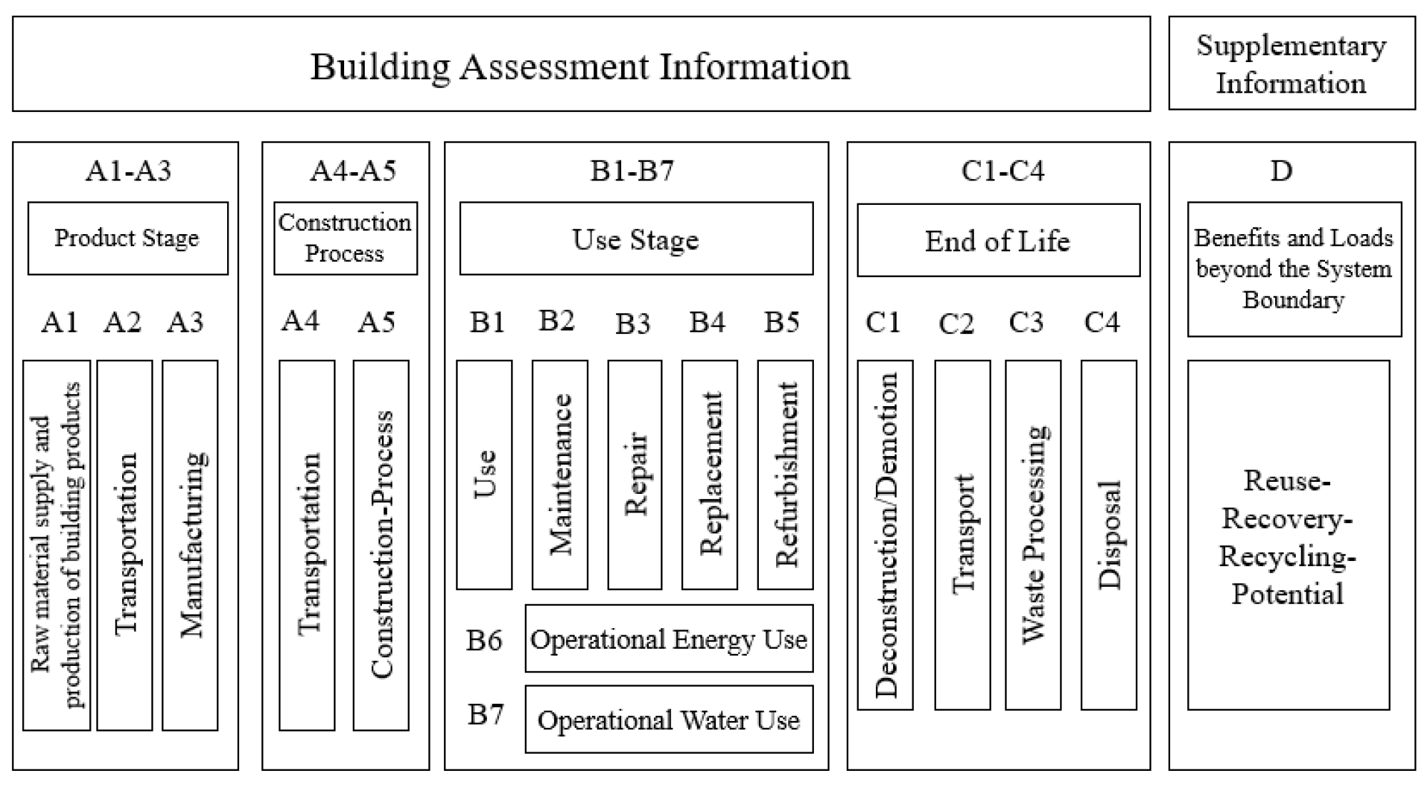
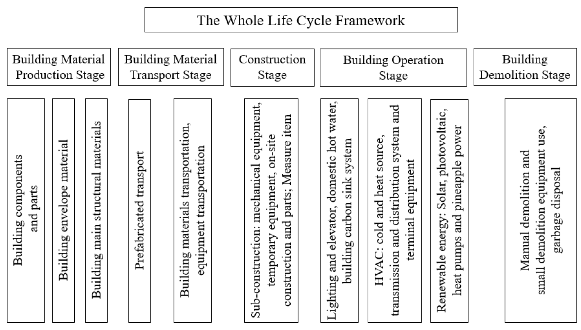
3.3. The Division of the Whole Life Cycle Framework of the Building

The whole life cycle assessment of buildings is developed from the life cycle assessment standards ISO 14040 and ISO 14044 [57]. This standard establishes the principles and framework of life cycle assessment, namely: (a) Definition of objectives and scope; (b) List analysis; (c) Impact assessment; (d) Explain. Building on these two standards, ISO 14067: 2018 guides and regulates the principles, requirements and guidelines for product carbon emissions [58]. The standard is characterized by an emphasis on setting the appropriate accounting scope for each product category. The European Committee for Standardization has proposed standards EN 15804:2019 and EN15978, which share the same modular concept (see Figure 1); both follow ISO 14040, and cover all life-cycle stages [59]. At present, the latest building life cycle classification standard adopted in China is GB 51336-2019 (see Figure 2), which divides the whole life cycle into five stages: production and transportation of building materials, construction, demolition, and operations. Compared with the EU classification standard, the domestic standard regards the transportation of building materials as a separate stage to reflect its importance. The default transport distance of other building materials is 500 km, except for the default transport distance of concrete which is 40 km [21].

4. Building Carbon Emission Prediction Model

At present, research on methods of predicting building carbon emissions is mainly based on the analysis of the leading factors of carbon emissions and then the establishment of various prediction models based on the leading factors, which can not only predict the carbon emission prospects of individual buildings, but also analyze the overall future carbon emission prospects of urban areas. The models can be divided into two categories: mathematical models, and machine learning models [60,61]. The regression model and the system dynamics model are the most widely used mathematical models [62]. See Table 4 for a detailed literature summary and model introduction.

4.1. Mathematical Model

The mathematical models used in the prediction of building carbon emissions include the factors decomposition model based on Kaya identity, various regression models, system dynamics model, grey system theory, and so on.

4.1.1. The Factor Decomposition Model Based on Kaya Identity

The Kaya identity was proposed by Japanese professor Yoyichi Kaya at an IPCC symposium in 1990 [63]:

$$C{O}_2=\frac{C{O}_2}{PE}\times \frac{PE}{GDP}\times \frac{GDP}{POP}\times POP=CI\times EI\times INC\times P$$

(4)

where CO₂, PE, GDP and POP are, respectively, carbon dioxide emissions, primary energy consumption, gross domestic product, and total population. Therefore, the influencing factors of carbon dioxide emissions are decomposed into emission coefficient factor (CI), energy intensity factor (EI), economic development factor (INC), and population factor (P).

This formula is currently the mainstream analysis method for decomposing and explaining the driving factors of carbon emissions. Its structure is simple, the factors are intuitive and quantifiable, and it can explain the driving factors of carbon emissions strongly. Since being proposed, it has been widely used in the fields of energy and environment [64]. However, the shortcoming of the Kaya identity is that the decomposition factors are limited to the relationship between CO₂ and population, energy, and economy. Therefore, researchers have successively proposed the IPAT decomposition method, STIRPAT model, LMDI decomposition method and other extended solutions based on Kaya identity [16,65,66].

1.

IPAT model

The IPAT equation, namely the environmental impact equation, was proposed by the scholar Ehrlich in the 1970s [67]:

$$I=PAT$$

(5)

The equation summed environmental impact (I) into the product of population (P), affluence (A), and technology (T). At present, researchers have mainly applied the model to study the effects of human activities on global warming, energy use, farmland degradation, carbon footprint, and pollution levels [68]. For example, Nie et al. [69] used the IPAT model to analyze the medium- and long-term economic growth, energy demand and carbon emission scenarios of Jiangsu Province, and introduced the main parameters and results of the three scenarios. Later, the researchers extended the IPAT model by adding other factors and proposed the IPBAT model [70], the ImPACT model [71], and the ImPACTS model [72]. However, the common shortcoming of these models is that they do not allow for hypothesis testing of missing items in the equation, and they also imply a linear assumption of the model that different variables have equal effects on the results, which is the biggest shortcoming of the model. To overcome this limitation, York et al. [73] reconstructed IPAT as a stochastic model, which they called the “STIRPAT model”.

2.

STIRPAT model

The extended STIRPAT model is an annotated form of the IPAT model with high convenience and application flexibility [15], that is:

$$I=a{P}^b{A}^c{T}^{d}e$$

(6)

where a is a constant term, b, c and d are the elastic coefficients of the three variables (P, A, and T), respectively, and e is the error term, representing a random variable that is not controllable or observable. In practice, the logarithm of the above formula is often taken into the following form:

$$\ln I=a+b\ln P+c\ln A+d\ln T+e$$

(7)

In view of the high versatility of the STIRPAT model, this model can be used to build a model of influencing factors of building carbon emissions, analyze the factors that have the greatest impact on building carbon emissions, and then further build a prediction model of building carbon emissions.

Table 4. Details of literature research on building carbon emission prediction model.

Author	Name	Characteristics
Nie et al. [69]	IPAT model	Reducing environmental change to the product of three interrelated driving forces, population, affluence, and technology. The disadvantage is that it does not allow hypothesis testing for missing items in the formula, and its extension model is commonly used, such as STIRPAT, etc.
Gu et al. [74]	LMDI model	Complete decomposition, no unexplained residuals, the results are more accurate, the widest range of use.
Zhou et al. [75]	MNR model	Regression analysis is simple and convenient, and suitable for preliminary analysis, but the equation assumptions are strict, “pseudo-regression” phenomena often appear, and large data samples are required. Often combined with STIRPAT, LMDI, and other factor decomposition models.
Sim [76]	System dynamics	It can effectively deal with nonlinear, complex and high-order practical problems, and can reflect the relationship between internal and external factors of the research object. It is especially good at dealing with long-term periodic and nonlinear complex system problems.
Wang and Gong [77]	Grey relational degree model	The degree of correlation between factors is judged according to the degree of similarity of the development trend of each factor, and there is no limit to whether there is any rule in the sample.
Li [78]	Grey GM (1,1) model	It requires less information, has high accuracy, is easy to check, and is very effective in dealing with small sample prediction problems.
Song and Zhang [79]	BP neural network	The nonlinear mapping ability is strong, it can approximate any continuous function, and it has the characteristics of adaptive learning and robust fault tolerance. However, the convergence rate of this model is slow and it may exhibit non-convergence and local minimum problems.
Hao and Gao [80]	NSGA-II-BP neural network	This algorithm can optimize the weight and threshold of the BP neural network, so as to improve the convergence speed of the latter.
Heydari et al. [81]	GWO-GRNNW	Grey wolf optimization mimics the hunting behavior and social leadership of the grey wolf. Different types of wolves assume different leadership levels, which can improve the spatial search efficiency.
Xu and Song [82]	FCS-SVM	The FCS algorithm avoids human influence when selecting kernel function type, kernel parameter, and penalty parameter in the SVM algorithm.
Wei et al. [83]	FOA-LSSVM	FOA is an intelligent optimization algorithm based on Drosophila foraging behavior. Combined with LSSVM, FOA can solve complex nonlinear mapping problems well.

Table 4. Details of literature research on building carbon emission prediction model.

Author	Name	Characteristics
Nie et al. [69]	IPAT model	Reducing environmental change to the product of three interrelated driving forces, population, affluence, and technology. The disadvantage is that it does not allow hypothesis testing for missing items in the formula, and its extension model is commonly used, such as STIRPAT, etc.
Gu et al. [74]	LMDI model	Complete decomposition, no unexplained residuals, the results are more accurate, the widest range of use.
Zhou et al. [75]	MNR model	Regression analysis is simple and convenient, and suitable for preliminary analysis, but the equation assumptions are strict, “pseudo-regression” phenomena often appear, and large data samples are required. Often combined with STIRPAT, LMDI, and other factor decomposition models.
Sim [76]	System dynamics	It can effectively deal with nonlinear, complex and high-order practical problems, and can reflect the relationship between internal and external factors of the research object. It is especially good at dealing with long-term periodic and nonlinear complex system problems.
Wang and Gong [77]	Grey relational degree model	The degree of correlation between factors is judged according to the degree of similarity of the development trend of each factor, and there is no limit to whether there is any rule in the sample.
Li [78]	Grey GM (1,1) model	It requires less information, has high accuracy, is easy to check, and is very effective in dealing with small sample prediction problems.
Song and Zhang [79]	BP neural network	The nonlinear mapping ability is strong, it can approximate any continuous function, and it has the characteristics of adaptive learning and robust fault tolerance. However, the convergence rate of this model is slow and it may exhibit non-convergence and local minimum problems.
Hao and Gao [80]	NSGA-II-BP neural network	This algorithm can optimize the weight and threshold of the BP neural network, so as to improve the convergence speed of the latter.
Heydari et al. [81]	GWO-GRNNW	Grey wolf optimization mimics the hunting behavior and social leadership of the grey wolf. Different types of wolves assume different leadership levels, which can improve the spatial search efficiency.
Xu and Song [82]	FCS-SVM	The FCS algorithm avoids human influence when selecting kernel function type, kernel parameter, and penalty parameter in the SVM algorithm.
Wei et al. [83]	FOA-LSSVM	FOA is an intelligent optimization algorithm based on Drosophila foraging behavior. Combined with LSSVM, FOA can solve complex nonlinear mapping problems well.

Lin et al. [84] decomposed CO₂ emissions into nine factors, such as population, urbanization employment level, and energy intensity. Combined with statistical data from 1991 to 2013, the STIRPAT model was used to analyze the effects of urbanization and real economic development on national CO₂ emissions. Based on the STIRPAT model, the grey correlation method, and neural networks, Zhang et al. [85] studied and predicted the carbon emissions of the construction industry in Jiangsu Province. The results showed that steel output, road transport distance, urbanization rate, and labor rate had a positive effect on the carbon emissions of the construction industry.

3.

The LMDI model

The traditional Divisia’s decomposition method has randomness in the parameter setting, which leads to residual errors in the decomposition results, and large residual errors affect the accuracy of the result analysis. LMDI decomposition is improved by Divisia’s decomposition method. For the complete mathematical principle, see [86]. The LMDI decomposition model is a complete decomposition without unexplained residuals, which makes the results more accurate. This model is now widely used in the analysis of building carbon emissions or building energy-influencing factors. For example, based on data on carbon emissions and GDP in Inner Mongolia from 1999 to 2009, Gong and Ji [87] used the LMDI model to study the carbon emission decomposition of six industries in Inner Mongolia, including the building industry, and evaluated the carbon emission driving intensity from the perspective of the total effect and industry. Chen et al. [88] combined spatial autocorrelation analysis, kernel density estimation, and the LMDI spatiotemporal model to analyze and study the driving factors of carbon emissions from urban residential buildings in 30 provinces of China during the period 2000–2019. Their results showed that residential area, population, and urbanization level were important driving factors affecting provincial carbon emissions. The above cases prove the application of the LMDI model in predicting the carbon emissions of the building industry

4.1.2. The Regression Model

The regression model is a mathematical model that quantitatively describes statistical relations and studies the relationship between dependent variables and independent variables. The regression equation is obtained by determining model parameters, and is used to predict changes in the trends of dependent variables. Some extended regression models, such as the double regression model, principal component regression model, multiple nonlinear regression model, multiple linear regression model, cubic polynomial model, etc., are mainly used in the actual prediction of building carbon emissions. At present, the carbon emission regression formula of the building demolition stage mostly adopts Zhang’s [89]:

$$C_{d1}=A\left(0.06X+2.01\right)$$

(8)

where, $C_{d1}$ is the carbon dioxide emissions in the demolition stage of the building, $A$ is the building area, and $X$ is the above-ground floor. After analyzing the embodied carbon emissions of 78 office buildings, Luo [90] proposed the following regression formula:

$$C_e=1.58x_1+378.97x_2+64.57x_3+94.19$$

(9)

where, $C_e$ is the embodied carbon emissions of the building, $x_1$ is the amount of steel used (kg), $x_2$ is the amount of concrete used (m³), and $x_3$ is the amount of wall materials used (m³).

In order to establish the carbon quota allocation plan for 2030, Zhou and Niu [75] used the double support vector regression model to forecast China’s provincial-level net carbon emissions during 2021–2030. Aiming at the carbon emission of residential buildings in Tianjin, Mao [17] used four models, including principal component regression analysis, to establish prediction models and engage in comparative analysis. When analyzing multi-factor models, regression models are simple, convenient, and suitable for preliminary analysis. However, the assumptions of regression equations are strict, and it is necessary to know all explanatory variables that cause the change of dependent variables. Otherwise, the problem of “pseudo-regression” can easily occur.

4.1.3. System Dynamics Model

System dynamics is a system simulation method proposed by Professor Forrester in 1956 to solve the problem of production management. It is a method to deepen analysis and solve problems step by step according to the idea of “qualitatively—quantitatively—qualitatively—model construction” [91]. Based on the idea that “system structure determines system function”, this method constructs a mathematical model according to the dependency between system behavior and internal mechanism, and seeks the root of the problem from the internal structure of the system. System dynamics can effectively solve nonlinear, complex and high-order practical problems, so it is widely used in the study of society, economics, and the environment. The framework of its modeling process is shown in Figure 3. Based on the system dynamics model, domestic and foreign scholars have carried out a lot of discussions on the subject of total carbon emission prediction and influencing factor analysis, which has played an important role in promoting the development of building carbon emissions. Based on the theory of system dynamics, Li et al. [92] established a prediction model considering the characteristics of regional energy consumption structure, and predicted the energy consumption structure of Liaoning Province during 2019–2038. With the help of system dynamics, Liu [93] explored the causal relationship and feedback mechanism of influencing factors on carbon emissions of prefabricated buildings, and predicted the changing trends of total carbon emissions and the effects of emission reduction. The advantage of system dynamics is that it can effectively deal with nonlinear, complex, and high-order practical problems, and can reflect the relationship between internal and external factors of the research object. It is especially good in dealing with long-term periodic and nonlinear complex system problems.

4.1.4. Grey System Theory

The grey relational degree model, developed from grey system theory, is a method to solve multi-factor and nonlinear problem analysis, which is often used in the selection of influencing factors. This method can make up for the shortcomings of requiring a large sample size (more than 30) in the systematic analysis of mathematical statistics such as regression analysis, and it has no limit on whether there is a rule of samples. Its basic idea is to judge the degree of correlation between factors according to the degree of similarity of the development trend of each factor. The influencing factors of building carbon emissions are often coupled, and the degree of influence of various factors is not obvious. Grey correlation analysis is often applied to this kind of situation.

The grey prediction model is a method to predict systems with uncertain factors. This method requires less information for modeling, has high precision, and is easy to check. It is very effective in dealing with small sample prediction problems. Since the grey prediction model is based on the first-order ordinary differential equation, it is also called the first-order unitary grey model, denoted as GM (1,1). Yue and Li [94] used the grey prediction model to predict the carbon emissions of hospital buildings in the whole life cycle, and conducted a quantitative analysis of carbon emissions at the hospital operation stage using dynamic analysis and static analysis. Based on the building model data series, Li et al. [78] used the GM (1.1) model to forecast the energy demand of Shandong Province from 2016 to 2020. The results showed that the energy demand of Shandong Province in 2020 increased by 20% compared with that in 2015.

The smooth implementation of building energy-saving and emission-reduction policies requires targeted improvement of leading carbon emission factors. Factor decomposition models, such as the IPAT model, STIRPAT model, and LMDI model based on Kaya identity, decompose the driving force of carbon emissions into leading factors, such as population and GDP. Then, according to the statistical data over the years, the carbon emission level of the city is predicted from a macro perspective. The main feature of this model is that it can clearly obtain the contribution rate of each factor to carbon emission, which is suitable for macro carbon emission analysis. The regression model is applicable to individual buildings at the microscopic level. It constructs regression formulas about major factors according to the statistical data of building carbon emissions. The regression formula is especially applicable in the initial stage of building design where the acquisition of data lists is scarce. The system dynamics model is a kind of model that deeply studies the relationship between internal and external factors in a system according to the idea of “system structure determines system function”. It is often used in conjunction with other prediction models. The grey relational degree model is a kind of model used to solve multi-factor and nonlinear problems. Compared with the regression model, this model is not limited by the number of samples, and requires less information to construct and has higher accuracy. Its application range is second only to the regression model.

4.2. Machine Learning Models

Machine learning models are widely used in the field of carbon emission prediction because of their characteristics of high precision, mature theory and low model cost. At present, the neural network model and the support vector machine model are the most used models.

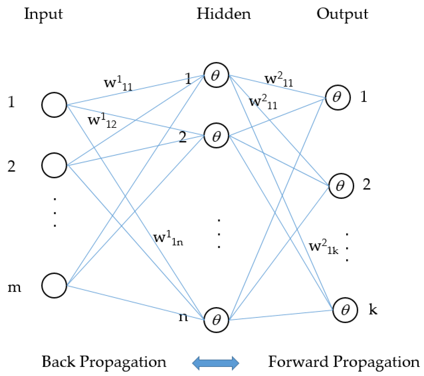
4.2.1. BP Neural Network

The back propagation (BP) neural network is a multi-layer feedforward neural network model trained according to the error back propagation algorithm. It is a black box model. As shown in Figure 4, the model includes three types of nodes: input layer nodes, output layer nodes, and hidden layer nodes. Each layer of neurons can communicate bidirectionally with the front and back neurons. The BP neural network has a strong nonlinear mapping ability, can approximate any continuous function, and has adaptive learning and robust fault tolerance characteristics, so it is widely used in the field of building carbon emission prediction, and is one of the most widely used neural network models. It is noteworthy that the BP neural network has problems of slow convergence, or even non-convergence and local minimum. Therefore, Hao and Gao [80] proposed an improved BP neural network based on the Non-dominated Sorting Genetic Algorithm-II (NSGA-II) genetic algorithm on the basis of the original model. The genetic algorithm is a multi-objective optimization algorithm, which can improve the convergence speed of the algorithm. Heydari et al. [81] proposed a generalized regression neural network based on the grey wolf optimization algorithm to predict carbon emissions, and the method was well applied to predict the carbon emissions of an Italian power grid.

4.2.2. The Support Vector Machine Model

Developed by Vapnik et al. [95] in 1995, the SVM model is a machine learning approach based on statistical learning theory. It can be divided into Support Vector Classification (SVC) and Support Vector Regression (SVR). The latter can be used for the study of regression equations between independent and dependent variables and is therefore widely used in predictive analysis, regression estimation, function approximation, etc. In theory, this method can obtain the global optimal solution, and has good generalization ability for unknown samples. It has significant advantages in solving small samples and nonlinear problems. The support vector machine model overcomes the shortcomings of low generalization ability and overfitting of neural networks and is considered an alternative to neural networks. Therefore, it is widely used in the prediction of carbon emissions in the construction industry. For example, Song [96] trained the support vector regression model with historical carbon emissions as samples and used it to forecast China’s carbon emissions from 2010 to 2015. However, the support vector machine model also has its own defects: the efficiency and performance of this method are affected by the type of kernel function, kernel parameter and penalty parameter, but these parameters are generally determined according to experience, which will lead to increased errors. Therefore, some scholars often combine the SVM algorithm with other algorithms. For example, Xu [82] used the SVM prediction model, optimized using the fuzzy cuckoo search (FCS) algorithm, to predict building carbon emissions, and used the FCS algorithm to search the parameters of the SVM algorithm to avoid the influence of human factors. Wei et al. [83] used the fruit fly algorithm to optimize the parameters of the least squares support vector machine, and predicted the carbon dioxide emissions from the optimized model.

The neural network method has a strong nonlinear fitting ability and can map any nonlinear relationship, which can result in a good prediction effect when building a complex carbon emission prediction model. However, the nature of the black box model of neural networks determines its poor portability. Compared with the neural network model, the support vector machine model has a more solid mathematical theoretical foundation, and has significant advantages in solving small samples and nonlinear problems. Currently, it is widely used in the field of carbon emission prediction.

In addition to the above models, there are other models with a smaller scope of application, which are not described in detail due to limited space, as shown in

Table 5. Details of literature research on some building carbon emission prediction models.

Author	Name	Characteristic
Zha et al. [97]	Divisia method	Compared with other factor decomposition methods, it has the unique advantages of zero residual error and uniform polymerization.
Feng and Wang [98]	Tapio decoupling model	It is often used to analyze the strength of the link between regional economic development and carbon emissions, which can be divided into three categories: “decoupling”, “linking” and “negative decoupling”.
Zhang [99]	LEAP model	The model is an ensemble model covering all sectors of energy consumption, production and energy use, which can be used to analyze urban energy demand and carbon emissions.
Ma et al. [100]	K-means clustering and logistic model	The K-means algorithm is easy to implement, simple, and has a fast clustering speed. The logistic algorithm is simple in calculation and has obvious economic significance. It can describe the growth of S-shaped curves.
Mansoor et al. [101]	LSTM	It has a strong approximation ability to nonlinear and non-stationary time series and is more accurate than BP neural network.

.

5. Conclusions and Perspectives

Countries are paying more attention to the problem of the worsening global climate caused by the increase in greenhouse gas emissions. In order to achieve the goal of carbon peaking and carbon neutrality, the construction industry is bound to make every effort to reduce energy consumption and greenhouse gas emissions from the perspective of the whole industry chain and the whole life cycle. All of these efforts are based on reliable and reasonable accounting of carbon emissions from the construction industry. With the correct accounting method, the carbon emissions of buildings, regions, cities, and even countries can be predicted so as to make overall planning easier and allow strategic adjustments to be made to the industrial structure and industrial development. For this purpose, this paper reviews the carbon emission accounting model and the prediction model.

• Carbon emission accounting methods can be divided into the carbon emission factor method, the mass balance method, and the measurement method. The carbon emission factor method is the main method recommended by IPCC, and is also the most widely used method at present. Although many countries and organizations have provided rich carbon emission factor databases for inquiry, the accuracy of carbon emission factor calculations using these databases is not good due to the poor timeliness or wide application range of the data contained in the databases. Therefore, supplementing and updating the carbon emission factor database is important work in the calculation of carbon emissions in various industries.
• Building carbon emission models are divided into the PB method, EI-O method, and hybrid method. Starting from the energy and material list of the building, the PB method calculates the carbon emissions of the whole building in detail, with high calculation accuracy but high cost. The EI-O method analyzes the carbon emissions of the whole building industry from a macro perspective, and is suitable for the analysis of carbon emissions at the city level. The hybrid method combines the advantages of the first two methods, and is the most widely used method at present.
• Research on the driving factors of carbon emission is mainly carried out using the STIPAT model, LMDI model, grey correlation degree, and other models. The main feature of these models is that the contribution rate of each factor to carbon emissions can be clearly obtained, and these models are suitable for carbon emission analysis at the level of industry and society.
• The prediction model is realized through mathematical models such as the regression model and the system dynamics model, as well as machine learning models such as the neural network model and the support vector machine model. In terms of application, various regression models, support vector machine models and their improved models are the research hotspots. However, in addition to the regression model, which is often used to predict the carbon emission of individual buildings, other commonly used prediction models mostly focus on the carbon emission prediction at the city or provincial level.

With the implementation of the “carbon peaking and carbon neutrality” policy and the implementation of the energy-saving emission reduction policy in the building industry, the accounting and prediction of building carbon emissions will become more and more important and common. At the level of model application, there are still the following problems:

• For the renewal and expansion of carbon emission factors, society should label the vast majority of products with carbon emission factors, similar to the “net content” label for every commodity. This work can be conducted by the manufacturer, so that the timeliness and details of the carbon emission factors can be addressed at the same time. The government should introduce corresponding compulsory measures and provide preferential policies to improve the enthusiasm of manufacturers.
• Most of the predictions of building carbon emissions in the literature focus on the macro level, and less attention is paid to predicting the carbon emissions of individual buildings, especially for prediction models in the building design stage. As the main model for predicting the embodied carbon emissions of single buildings, the accuracy of the regression model requires a large amount of measured data as the analysis basis, but it is difficult to obtain complete and effective measured data, which requires further accumulation by researchers.

References

1. Kabir, M.; Habiba, U.E.; Khan, W.; Shah, A.; Rahim, S.; Rios-Escalante, P.R.D.l.; Farooqi, Z.-U.-R.; Ali, L.; Shafiq, M. Climate change due to increasing concentration of carbon dioxide and its impacts on environment in 21st century; a mini review. J. King Saud Univ.-Sci. 2023, 35, 102693. [Google Scholar] [CrossRef]
2. Webster, M.D.; Meryman, H.; Kestner, D.M. Carbon emissions and building structure: What the structural engineer needs to know about carbon in the 21st century. Proc. Struct. Congr. 2011, 2011, 472–482. [Google Scholar]
3. Li, R.; Kang, L.; Wu, S.; Zhou, X.; Wang, X. Effect of dust formation on the fate of indoor phthalates: Model analysis. Build. Environ. 2023, 229, 109957. [Google Scholar] [CrossRef]
4. Atmaca, A.; Atmaca, N. Carbon footprint assessment of residential buildings, a review and a case study in Turkey. J. Clean Prod. 2022, 340, 130691. [Google Scholar] [CrossRef]
5. Wang, Z.; Wang, F.; Liu, J.; Li, Y.; Wang, M.; Luo, Y.; Ma, L.; Zhu, C.; Cai, W. Energy analysis and performance assessment of a hybrid deep borehole heat exchanger heating system with direct heating and coupled heat pump approaches. Energy Convers. Manag. 2023, 276, 116484. [Google Scholar] [CrossRef]
6. Purohit, P.; Borgford-Parnell, N.; Klimont, Z.; Höglund-Isaksson, L. Achieving Paris climate goals calls for increasing ambition of the Kigali Amendment. Nat. Clim. Change 2022, 12, 339–342. [Google Scholar] [CrossRef]
7. Rajamani, L.; Werksman, J. The legal character and operational relevance of the Paris Agreement’s temperature goal. Philos. Trans. A Math Phys. Eng. Sci. 2018, 376, 0458. [Google Scholar] [CrossRef] [PubMed] [Green Version]
8. Torjesen, I. Paris Agreement’s ambition to limit global warming to 1.5 degrees C still possible, analysis shows. BMJ 2017, 358, j4332. [Google Scholar] [CrossRef] [PubMed]
9. Musah, M.; Gyamfi, B.A.; Kwakwa, P.A.; Agozie, D.Q. Realizing the 2050 Paris climate agreement in West Africa: The role of financial inclusion and green investments. J. Environ. Manag. 2023, 340, 117911. [Google Scholar] [CrossRef] [PubMed]
10. Peng, C.H. Calculation of a building’s life cycle carbon emissions based on Ecotect and building information modeling. J. Clean Prod. 2016, 112, 453–465. [Google Scholar] [CrossRef]
11. Harish, V.S.K.V.; Kumar, A. A review on modeling and simulation of building energy systems. Renew. Sust. Energ. Rev. 2016, 56, 1272–1292. [Google Scholar] [CrossRef]
12. Zhu, C.; Li, X.; Zhu, W.; Gong, W. Embodied carbon emissions and mitigation potential in China’s building sector: An outlook to 2060. Energy Policy 2022, 170, 113222. [Google Scholar] [CrossRef]
13. Zhang, Y.; Yan, D.; Hu, S.; Guo, S. Modelling of energy consumption and carbon emission from the building construction sector in China, a process-based LCA approach. Energy Policy 2019, 134, 110949. [Google Scholar] [CrossRef]
14. Zhou, B.; Li, Y.; Ding, Y.; Huang, G.; Shen, Z. An input-output-based Bayesian neural network method for analyzing carbon reduction potential: A case study of Guangdong province. J. Clean Prod. 2023, 389, 135986. [Google Scholar] [CrossRef]
15. Yu, S.; Zhang, Q.; Hao, J.L.; Ma, W.; Sun, Y.; Wang, X.; Song, Y. Development of an extended STIRPAT model to assess the driving factors of household carbon dioxide emissions in China. J. Environ. Manag. 2023, 325, 116502. [Google Scholar] [CrossRef]
16. Ma, M.; Cai, W.; Cai, W. Carbon abatement in China’s commercial building sector: A bottom-up measurement model based on Kaya-LMDI methods. Energy 2018, 165, 350–368. [Google Scholar] [CrossRef]
17. Xikai, M.; Lixiong, W.; Jiwei, L.; Xiaoli, Q.; Tongyao, W. Comparison of regression models for estimation of carbon emissions during building’s lifecycle using designing factors: A case study of residential buildings in Tianjin, China. Energy Build. 2019, 204, 109519. [Google Scholar] [CrossRef]
18. Nie, W.; Duan, H. A novel multivariable grey differential dynamic prediction model with new structures and its application to carbon emissions. Eng. Appl. Artif. Intell. 2023, 122, 106174. [Google Scholar] [CrossRef]
19. Wang, P.; Hu, J.; Chen, W. A hybrid machine learning model to optimize thermal comfort and carbon emissions of large-space public buildings. J. Clean Prod. 2023, 400, 136538. [Google Scholar] [CrossRef]
20. Yang, H.; Wang, M.; Li, G. A combined prediction model based on secondary decomposition and intelligence optimization for carbon emission. Appl. Math. Model. 2023, 121, 484–505. [Google Scholar] [CrossRef]
21. GB/T 51366-2019; Standard for Building Carbon Emission Calculation. Ministry of Housing and Urban-Rural Development: Beijing, China, 2019.
22. Li, X.; Xie, Y.; Li, C.; Wang, Z.; Hopke, P.K.; Xue, C. Using the carbon balance method based on fuel-weighted average concentrations to estimate emissions from household coal-fired heating stoves. Chemosphere 2022, 307, 135639. [Google Scholar] [CrossRef]
23. Yona, L.; Cashore, B.; Jackson, R.B.; Ometto, J.; Bradford, M.A. Refining national greenhouse gas inventories. Ambio 2020, 49, 1581–1586. [Google Scholar] [CrossRef] [Green Version]
24. Chen, Y.; Fang, Y.; Feng, W.; Zhang, Y.; Zhao, G.X. How to minimise the carbon emission of steel building products from a cradle-to-site perspective: A systematic review of recent global research. J. Clean Prod. 2022, 368, 133156. [Google Scholar] [CrossRef]
25. Lai, K.E.; Abdul Rahiman, N.; Othman, N.; Ali, K.N.; Lim, Y.W.; Moayedi, F.; Mat Dzahir, M.A. Quantification process of carbon emissions in the construction industry. Energy Build. 2023, 289, 113025. [Google Scholar] [CrossRef]
26. Zhao, Y.; Liu, L.; Yu, M. Comparison and analysis of carbon emissions of traditional, prefabricated, and green material buildings in materialization stage. J. Clean Prod. 2023, 406, 137152. [Google Scholar] [CrossRef]
27. Wong, J.K.W.; Zhou, J. Enhancing environmental sustainability over building life cycles through green BIM: A review. Autom. Constr. 2015, 57, 156–165. [Google Scholar] [CrossRef]
28. Mao, C.; Shen, Q.; Shen, L.; Tang, L. Comparative study of greenhouse gas emissions between off-site prefabrication and conventional construction methods: Two case studies of residential projects. Energy Build. 2013, 66, 165–176. [Google Scholar] [CrossRef] [Green Version]
29. Greene, J.M.; Hosanna, H.R.; Willson, B.; Quinn, J.C. Whole life embodied emissions and net-zero emissions potential for a mid-rise office building constructed with mass timber. Sustain. Mater. Technol. 2023, 35, e00528. [Google Scholar] [CrossRef]
30. Pajchrowski, G.; Noskowiak, A.; Lewandowska, A.; Strykowski, W. Wood as a building material in the light of environmental assessment of full life cycle of four buildings. Constr. Build. Mater. 2014, 52, 428–436. [Google Scholar] [CrossRef]
31. Cai, B.; Zhang, L.; Xia, C.; Yang, L.; Liu, H.; Jiang, L.; Cao, L.; Lei, Y.; Yan, G.; Wang, J. A new model for China’s CO2 emission pathway using the top-down and bottom-up approaches. Chin. J. Popul. Resour. Environ. 2021, 19, 291–294. [Google Scholar] [CrossRef]
32. van Vuuren, D.P.; Hoogwijk, M.; Barker, T.; Riahi, K.; Boeters, S.; Chateau, J.; Scrieciu, S.; van Vliet, J.; Masui, T.; Blok, K.; et al. Comparison of top-down and bottom-up estimates of sectoral and regional greenhouse gas emission reduction potentials. Energy Policy 2009, 37, 5125–5139. [Google Scholar] [CrossRef]
33. Zhang, X.; Wang, F. Hybrid input-output analysis for life-cycle energy consumption and carbon emissions of China’s building sector. Build. Environ. 2016, 104, 188–197. [Google Scholar] [CrossRef]
34. Zhang, X.; Wang, F. Assessment of embodied carbon emissions for building construction in China: Comparative case studies using alternative methods. Energy Build. 2016, 130, 330–340. [Google Scholar] [CrossRef]
35. Zhang, X.; Liu, K.; Zhang, Z. Life cycle carbon emissions of two residential buildings in China: Comparison and uncertainty analysis of different assessment methods. J. Clean Prod. 2020, 266, 122037. [Google Scholar] [CrossRef]
36. Anny, H.Y.; Weber, C.L.; Scott, M.H. Categorization of scope 3 emissions for streamlined enterprise carbon footprinting. Environ. Sci. Technol. 2009, 43, 8509–8515. [Google Scholar] [CrossRef] [Green Version]
37. Van Ooteghem, K.; Xu, L. The life-cycle assessment of a single-storey retail building in Canada. Build. Environ. 2012, 49, 212–226. [Google Scholar] [CrossRef] [Green Version]
38. Gerilla, G.P.; Teknomo, K.; Hokao, K. An environmental assessment of wood and steel reinforced concrete housing construction. Build. Environ. 2007, 42, 2778–2784. [Google Scholar] [CrossRef]
39. Shao, L.; Chen, G.Q.; Chen, Z.M.; Guo, S.; Han, M.Y.; Zhang, B.; Hayat, T.; Alsaedi, A.; Ahmad, B. Systems accounting for energy consumption and carbon emission by building. Commun. Nonlinear Sci. Numer. Simul. 2014, 19, 1859–1873. [Google Scholar] [CrossRef]
40. Acquaye, A.A.; Duffy, A.P. Input–output analysis of Irish construction sector greenhouse gas emissions. Build. Environ. 2010, 45, 784–791. [Google Scholar] [CrossRef] [Green Version]
41. Biswas, W.K. Carbon footprint and embodied energy consumption assessment of building construction works in Western Australia. Int. J. Sustain. Built Environ. 2014, 3, 179–186. [Google Scholar] [CrossRef] [Green Version]
42. Wang, Y.; Wang, W.; Mao, G.; Cai, H.; Zuo, J.; Wang, L.; Zhao, P. Industrial CO2 emissions in China based on the hypothetical extraction method: Linkage analysis. Energy Policy 2013, 62, 1238–1244. [Google Scholar] [CrossRef]
43. Yu, D.; Tan, H.; Ruan, Y. A future bamboo-structure residential building prototype in China: Life cycle assessment of energy use and carbon emission. Energy Build. 2011, 43, 2638–2646. [Google Scholar] [CrossRef]
44. Cuéllar-Franca, R.M.; Azapagic, A. Environmental impacts of the UK residential sector: Life cycle assessment of houses. Build. Environ. 2012, 54, 86–99. [Google Scholar] [CrossRef]
45. Dong, H.; Geng, Y.; Fujita, T.; Jacques, D.A. Three accounts for regional carbon emissions from both fossil energy consumption and industrial process. Energy 2014, 67, 276–283. [Google Scholar] [CrossRef]
46. Monahan, J.; Powell, J.C. An embodied carbon and energy analysis of modern methods of construction in housing: A case study using a lifecycle assessment framework. Energy Build. 2011, 43, 179–188. [Google Scholar] [CrossRef]
47. You, F.; Hu, D.; Zhang, H.; Guo, Z.; Zhao, Y.; Wang, B.; Yuan, Y. Carbon emissions in the life cycle of urban building system in China—A case study of residential buildings. Ecol. Complex. 2011, 8, 201–212. [Google Scholar] [CrossRef]
48. Chang, Y.; Ries, R.J.; Wang, Y. The embodied energy and environmental emissions of construction projects in China: An economic input–output LCA model. Energy Policy 2010, 38, 6597–6603. [Google Scholar] [CrossRef]
49. Yan, H.; Shen, Q.; Fan, L.C.H.; Wang, Y.; Zhang, L. Greenhouse gas emissions in building construction: A case study of One Peking in Hong Kong. Build. Environ. 2010, 45, 949–955. [Google Scholar] [CrossRef] [Green Version]
50. Nässén, J.; Holmberg, J.; Wadeskog, A.; Nyman, M. Direct and indirect energy use and carbon emissions in the production phase of buildings: An input–output analysis. Energy 2007, 32, 1593–1602. [Google Scholar] [CrossRef]
51. Li, D.Z.; Chen, H.X.; Hui, E.C.M.; Zhang, J.B.; Li, Q.M. A methodology for estimating the life-cycle carbon efficiency of a residential building. Build. Environ. 2013, 59, 448–455. [Google Scholar] [CrossRef]
52. Leontief, W. Input-Output-Analysis—Foreword. Reg. Sci. Urban Econ. 1994, 24, 1. [Google Scholar] [CrossRef]
53. Bullard, C.W.; Penner, P.S.; Pilati, D.A. Net energy analysis: Handbook for combining process and input-output analysis. Resour. Energy 1978, 1, 267–313. [Google Scholar] [CrossRef]
54. Zhang, L.X.; Wang, C.B.; Song, B. Carbon emission reduction potential of a typical household biogas system in rural China. J. Clean Prod. 2013, 47, 415–421. [Google Scholar] [CrossRef]
55. Peters, G.P. Carbon footprints and embodied carbon at multiple scales. Curr. Opin. Environ. Sustain. 2010, 2, 245–250. [Google Scholar] [CrossRef]
56. Sangwon, S.; Manfred, L.; Treloar, G.; Hiroki, H.; Arpad, H.; Gjalt, H. System boundary selection in life-cycle inventoried using hybrid approaches. Environ. Sci. Technol. 2004, 38, 657–664. [Google Scholar] [CrossRef]
57. de Lassio, J.; Franca, J.; Espirito Santo, K.; Haddad, A. Case study: LCA methodology applied to materials management in a Brazilian residential construction site. J. Eng. 2016, 2016, 8513293–8513299. [Google Scholar] [CrossRef] [Green Version]
58. Fort, J.; Cerny, R. Carbon footprint analysis of calcined gypsum production in the Czech Republic. J. Clean Prod. 2018, 177, 795–802. [Google Scholar] [CrossRef]
59. Hoxha, E.; Passer, A.; Mendes Saade, M.; Trigaux, D.; Shuttleworth, A.; Pittau, F.; Allacker, K.; Habert, G. Biogenic carbon in buildings: A critical overview of LCA methods. Build. Cities 2020, 1, 504–524. [Google Scholar] [CrossRef]
60. Sun, W.; Wang, Y.; Zhang, C. Forecasting CO2 emissions in Hebei, China, through moth-flame optimization based on the random forest and extreme learning machine. Environ. Sci. Pollut. Res. 2018, 25, 28985–28997. [Google Scholar] [CrossRef]
61. Pan, W.; Li, K.; Teng, Y. Rethinking system boundaries of the life cycle carbon emissions of buildings. Renew. Sust. Energ. Rev. 2018, 90, 379–390. [Google Scholar] [CrossRef]
62. Fang, Y.; Lu, X.; Li, H. A random forest-based model for the prediction of construction-stage carbon emissions at the early design stage. J. Clean Prod. 2021, 328, 129657. [Google Scholar] [CrossRef]
63. Kaya, Y. Impact of carbon dioxide emission on GNP growth: Interpretation of proposed scenarios. In Response Strategies Working Group Report 1989; IPCC: Geneva, Switzerland, 1989. [Google Scholar]
64. Lu, Y.; Jiahua, P. Disaggregation of carbon emission drivers in Kaya identity and its limitations with regard to policy implications. Adv. Clim. Change Res. 2013, 9, 210. [Google Scholar]
65. Yang, J.; Song, K.; Hou, J.; Zhang, P.; Wu, J. Temporal and spacial dynamics of bioenergy-related CO 2 emissions and underlying forces analysis in China. Renew. Sustain. Energy Rev. 2017, 70, 1323–1330. [Google Scholar] [CrossRef]
66. Li, J.; Chen, Y.; Li, Z.; Liu, Z. Quantitative analysis of the impact factors of conventional energy carbon emissions in Kazakhstan based on LMDI decomposition and STIRPAT model. J. Geogr. Sci. 2018, 28, 1001–1019. [Google Scholar] [CrossRef] [Green Version]
67. Ehrlich, P.R.; Holdren, J.P. Critique. Bull. At. Sci. 1972, 28, 16–27. [Google Scholar] [CrossRef]
68. York, R.; Rosa, E.A.; Dietz, T. A rift in modernity? Assessing the anthropogenic sources of global climate change with the STIRPAT model. Int. J. Sociol. Soc. Policy 2003, 23, 31–51. [Google Scholar] [CrossRef]
69. Nie, R.; Zhang, T.; Wang, D. The scenario analysis on energy consumption and carbon emissions based on environmental loads model. J. Nat. Resour. 2010, 9, 1557–1564. [Google Scholar]
70. Schulze, P.C. I = PAT. Ecol. Econ. 2002, 40, 149–150. [Google Scholar] [CrossRef]
71. Waggoner, P.E.; Ausubel, J.H. A framework for sustainability. Proc. Natl. Acad. Sci. USA 2002, 99, 7860–7865. [Google Scholar] [CrossRef] [PubMed] [Green Version]
72. Xu, Z.; Cheng, G.; Qiu, G. ImPACTS identity of sustainability assessment. Acta Geogr. Sin. 2005, 60, 198–208. [Google Scholar]
73. York, R.; Rosa, E.A.; Dietz, T. STIRPAT, IPAT and ImPACT: Analytic tools for unpacking the driving forces of environmental impacts. Ecol. Econ. 2003, 46, 351–365. [Google Scholar] [CrossRef]
74. Gu, S.; Fu, B.; Thriveni, T.; Fujita, T.; Ahn, J.W. Coupled LMDI and system dynamics model for estimating urban CO2 emission mitigation potential in Shanghai, China. J. Clean Prod. 2019, 240, 118034. [Google Scholar] [CrossRef]
75. Zhou, X.; Niu, A.; Lin, C. Optimizing carbon emission forecast for modelling China’s 2030 provincial carbon emission quota allocation. J. Environ. Manag. 2023, 325, 116523. [Google Scholar] [CrossRef] [PubMed]
76. Sim, J.; Sim, J. The effect of new carbon emission reduction targets on an apartment building in South Korea. Energy Build. 2016, 127, 637–647. [Google Scholar] [CrossRef]
77. Wang, L.-p.; Gong, G.-c. Energy consumption and carbon emission analysis of residential building materials preparation stage based on grey system theory: A case study of Hefei. J. Hunan Univ. (Nat. Sci.) 2016, 43, 151–156. [Google Scholar]
78. Li, S.; Li, R. Comparison of Forecasting Energy Consumption in Shandong, China Using the ARIMA Model, GM Model, and ARIMA-GM Model. Sustainability 2017, 9, 1181. [Google Scholar] [CrossRef] [Green Version]
79. Jiekun, S.; Yu, Z. Scene predicion of china’s carbon emisisons based on BP neural network. Sci. Teechonology Eng. 2011, 11, 4108–4112. [Google Scholar]
80. Hao, J.-y.; Gao, J. Prediction Model of Urban Building Carbon Emissions and Reduction Based on the BP Neural Network Improved by NSGA- II. Build. Energy Effic. 2016, 44, 122–124. [Google Scholar] [CrossRef]
81. Heydari, A.; Garcia, D.A.; Keynia, F.; Bisegna, F.; De Santoli, L. Renewable energies generation and carbon dioxide emission forecasting in microgrids and national grids using GRNN-GWO methodology. Energy Procedia 2019, 159, 154–159. [Google Scholar] [CrossRef]
82. Xu, Y.; Song, W. Carbon Emission Prediction of Construction Industry Based on FCS-SVM. Ecol. Econ. 2019, 35, 37–41. [Google Scholar]
83. Wei, S.; Wang, T.; Li, Y. Influencing factors and prediction of carbon dioxide emissions using factor analysis and optimized least squares support vector machine. Environ. Eng. Res. 2017, 22, 175–185. [Google Scholar] [CrossRef]
84. Lin, S.; Wang, S.; Marinova, D.; Zhao, D.; Hong, J. Impacts of urbanization and real economic development on CO2 emissions in non-high income countries: Empirical research based on the extended STIRPAT model. J. Clean Prod. 2017, 166, 952–966. [Google Scholar] [CrossRef]
85. Zhang, S.; Huo, Z.; Zhai, C. Building Carbon Emission Scenario Prediction Using STIRPAT and GA-BP Neural Network Model. Sustainability 2022, 14, 9369. [Google Scholar] [CrossRef]
86. Ang, B.W. The LMDI approach to decomposition analysis: A practical guide. Energy Policy 2005, 33, 867–871. [Google Scholar] [CrossRef]
87. Gong, F.; Wang, F. Carbon emissions in Inner Mongolia. J. Arid Land Resour. Environ. 2013, 27, 36–40. [Google Scholar]
88. Chen, H.; Du, Q.; Huo, T.; Liu, P.; Cai, W.; Liu, B. Spatiotemporal patterns and driving mechanism of carbon emissions in China’s urban residential building sector. Energy 2023, 263, 126102. [Google Scholar] [CrossRef]
89. Zhang, J.; Yan, Z.; Bi, W.; Ni, P.; Lei, F.; Yao, S.; Lang, J. Prediction and scenario simulation of the carbon emissions of public buildings in the operation stage based on an energy audit in Xi’an, China. Energy Policy 2023, 173, 113396. [Google Scholar] [CrossRef]
90. Luo, Z.; Yang, L.; Liu, J. Carbon dioxide emissions of office buildings at embodied stage. J. Civ. Archit. Environ. Eng. 2014, 36, 37–43. [Google Scholar] [CrossRef]
91. Forrester, J.W. System dynamics—A personal view of the first fifty years. Syst. Dyn. Rev. 2007, 23, 345–358. [Google Scholar] [CrossRef]
92. Li, H.Y.; Li, B.; Niu, D.X. Prediction on the Energy Consumption Structure in Liaoning Province Based on System Dynamics. Pol. J. Environ. Stud. 2021, 30, 5593–5604. [Google Scholar] [CrossRef]
93. Ying, L. Research on Carbon Emission of Prefabricated Buildings Based on System Dynamics Simulation. Master’s Thesis, Yantai University, Shandong, China, 2021. [Google Scholar]
94. Yue, J.J.; Li, W.R.; Cheng, J.; Xiong, H.X.; Xue, Y.; Deng, X.; Zheng, T.H. A dynamic calculation model of the carbon footprint in the life cycle of hospital building: A case study in China. Eng. Constr. Archit. Manag. 2022; ahead of print. [Google Scholar] [CrossRef]
95. Cortes, C.; Vapnik, V. Support-vector networks. Mach. Learn. 1995, 20, 273–297. [Google Scholar] [CrossRef]
96. Song, J.-k. China’s carbon emissions prediction model based on support vector regression. J. China Univ. Pet. 2012, 36, 182–187. [Google Scholar] [CrossRef]
97. Jianping, Z.; Fangfang, T.; Hao, F. Empirical study of energy-induced carbon emissions in china industries based on Divisia decomposition approach: An industry view. Mod. Econ. Sci. 2010, 32, 88–94. [Google Scholar]
98. Feng, B.; Wang, X. Research on carbon decoupling effect and influence factors of provincial construction industry in China. China Popul. Resour. Env. 2015, 25, 28–34. [Google Scholar]
99. Zhang, W. Study on Carbon Emission Simulation of Civil Construction Operation Period in Jilin Province Based on LEAP. Master’s Thesis, Jilin University, Changchun, China, 2017. [Google Scholar]
100. Ma, L.; Lin, K.; Guan, M.; Lin, M. The prediction of carbon emission in all provinces of China with the K-means cluster based Logistic model. In Proceedings of the 2017 International Conference on Service Systems and Service Management, Dalian, China, 16–18 June 2017; pp. 1–6. [Google Scholar]
101. Ahmed, M.; Shuai, C.; Ahmed, M. Influencing factors of carbon emissions and their trends in China and India: A machine learning method. Environ. Sci. Pollut. Res. 2022, 29, 48424–48437. [Google Scholar] [CrossRef]
Figure 1. System boundaries according to EN 15804/EN 15978.
Buildings 13 01617 g001
Figure 2. The whole life cycle framework of ‘Standard for building carbon emission calculation’.
Buildings 13 01617 g002
Figure 3. Modeling process of System dynamics model.
Buildings 13 01617 g003
Figure 4. Neural network structure principle.
Buildings 13 01617 g004