Article

Bayesian Model-Updating Implementation in a Five-Story Building

1
School of Civil Engineering and Geomatics, Universidad del Valle, Cali 760032, Colombia
2
Facultad de Ingeniería y Ciencias Aplicadas, Universidad de los Andes, Santiago 7620001, Chile
*
Author to whom correspondence should be addressed.
Buildings 2023, 13(6), 1568; https://doi.org/10.3390/buildings13061568
Submission received: 24 April 2023 / Revised: 8 June 2023 / Accepted: 16 June 2023 / Published: 20 June 2023

Abstract

:
Simplifications and theoretical assumptions are usually incorporated into the numerical modeling of structures. However, these assumptions may reduce the accuracy of the simulation results. This problem has led to the development of model-updating techniques to minimize the error between the experimental response and the modeled structure by updating its parameters based on the observed data. Structural numerical models are typically constructed using a deterministic approach, whereby a single best-estimated value of each structural parameter is obtained. However, structural models are often complex and involve many uncertain variables, where a unique solution that captures all the variability is not possible. Updating techniques using Bayesian Inference (BI) have been developed to quantify parametric uncertainty in analytical models. This paper presents the implementation of the BI in the parametric updating of a five-story building model and the quantification of its associated uncertainty. The Bayesian framework is implemented to update the model parameters and calculate the covariance matrix of the output parameters based on the experimental information provided by modal frequencies and mode shapes. The main advantage of this approach is that the uncertainty in the experimental data is considered by defining the likelihood function as a multivariate normal distribution, leading to a better representation of the actual building behavior. The results showed that this Bayesian model-updating approach effectively allows a statistically rigorous update of the model parameters, characterizing the uncertainty and increasing confidence in the model’s predictions, which is particularly useful in engineering applications where model accuracy is critical.

1. Introduction

Commonly, the mechanical behavior of infrastructure systems is determined through analytical methods, experimental testing, and field observations. In structural engineering, modeling uses mathematical and computational techniques to simulate the mechanical behavior under different load conditions. Deterministic mathematical models are widely adopted to accurately represent the behavior of real structures while avoiding excessive computational costs. These models are favored for their ease of manipulation; however, their accuracy in representing the real behavior of built structures is often limited [1,2]. Therefore, the model-updating methodology attempts to decrease the gap between the constructed structural system and its structural model’s behavior [3].
The Finite Element Method (FEM) has been extensively applied in structural engineering [4]. The traditional approach to estimating the parameters of an FE model is based on a unique result for a given set of inputs, no matter how many times it is recalculated. This deterministic modeling approach limits the information obtained from experimental data, since the uncertainty associated with each structural parameter is not included in the analysis [5]. The uncertainty might arise from a combination of factors, including lack of knowledge, material variability, load changes, measurement errors, and modeling assumptions [6,7,8]. Over the years, significant contributions have been made towards incorporating uncertainty in structural models and their parameters, aiming to update building code models [9].
The uncertainty may be accounted for using probabilistic methods when statistical distributions are incorporated, providing more realistic estimations of the structural response. Inferential statistics proposes an alternative solution to the deterministic approach by generating models where the results are given probabilistically. Thus, it is possible to know how accurate the model outputs are, draw conclusions based on percentages, and make decisions to develop safer designs [10]. Parametric updating of structural models often implements the Bayesian over other probabilistic approaches due to the incorporation of prior knowledge. This technique provides more accurate parameter estimation by accounting for uncertainty and updating beliefs as new information is obtained. Additionally, it provides a systematic framework for model selection and is able to handle complex and nonlinear models. Thus, valuable experimental information should be obtained to feed the models to be updated. Many structural identification methods typically rely on a deterministic approach, which involves experimental measurement of properties and estimating unknown or non-measurable model parameters by minimizing an error function based on these measurements. With this deterministic approach, the information obtained from tests is limited to the measurements taken and their accuracy, and there is no consideration of uncertainty or variability in the measurements. On the other hand, probabilistic approaches such as Bayesian updating take into account uncertainty in the model parameters and incorporate prior knowledge, which may lead to more accurate and robust parameter estimation.
Ambient vibration testing is a useful and non-destructive method for measuring the response of a structure, allowing the estimation of modal parameters. The Bayesian Inference (BI) approach proposes a methodology to quantify the uncertainty associated with the model and its input parameters. The information obtained from experimental tests is augmented using a Bayesian-approached model to quantify the uncertainty in the data [11]. However, implementing Bayesian model updating with FE models is still challenging. Updating the model parameters using Bayesian methods requires evaluating functions multiple times, which might be computationally expensive when dealing with large FE models. Nonetheless, the development of efficient computational methods and algorithms continues to advance the application of Bayesian model updating in the field of structural engineering [12,13].
This paper aims to implement the BI framework for the parametric updating of a structural FE model based on experimental modal properties. The methodology proposes quantifying the model’s uncertainty taking into account different kinds of observations using a multivariate normal likelihood function. The reference structure for implementing the developed method is a full-scale five-story reinforced concrete building. Specialized software for performing Bayesian updating of a complex model is utilized. Furthermore, the software allows cloud-based computational solutions and other techniques to make the updating process of this computationally expensive model feasible and valuable.
This specific research holds a remarkable significance in the field due to the incorporation of two innovative approaches: the utilization of test data and the implementation of iterative calculation of the covariance matrix. The research conducted by Loyola (2018) [14] highlights that the architecture, engineering, construction, and operation (AECO) industry lags behind in harnessing the potential of big data compared to other sectors. With limited examples and a lack of practical application, the use of data and Bayesian models in this study brings a significant contribution to decision-making processes in building design. Furthermore, the comparison between the iterative calculation of the covariance matrix and the use of an identity matrix as covariance matrix in the paper represents a significant disclosure within the field, contributing valuable insights and paving the way for further developments.
The organization of this paper is as follows. The Introduction provides an overview of the research topic and an explanation of its significance. Section 2 presents the Bayesian inference framework. Section 3 describes the experimental program, including the characteristics of the reference structure and data collection. In Section 4, the implementation of Bayesian inference in the parametric updating of the reference structure model using identified modal properties is presented. The results are presented in Section 5, which involves assessing the behavior of various parametric uncertainties and evaluating the predictive performance of the updated structural model. Finally, the main findings are discussed and the potential implications of the implementation of this framework are considered in the Conclusions.

2. BI in Finite Element Model Updating (FEMU)

A comprehensive understanding of the BI methodology employed in this study requires specific concepts explained in [15,16,17]. Uncertainty in modeling complex systems may be classified as epistemic or aleatory. Epistemic uncertainty arises from a lack of knowledge and might be reduced through improved data and modeling, while aleatory uncertainty results from inherent variability or randomness and cannot be reduced. Therefore, it is the epistemic error that we aim to reduce through the implementation of BI in structural models. BI is based on Bayes’ theorem [18], which is defined as:
P ( A B ) = P ( B A ) · P ( A ) P ( B )
where P ( A | B ) is the conditional probability of event A given event B has occurred, P ( B | A ) is the conditional probability of event B given event A has occurred, P ( A ) is the prior probability of event A, P ( B ) is the prior probability of event B.
Bayes’ theorem is based on the fundamental principle where laws of probability guide rational belief. In BI, the probabilities represent degrees of belief rather than frequencies or long-term averages. This methodology provides a framework for updating beliefs as more experimental evidence or information becomes available, starting with prior beliefs and using Bayes’ rule to derive a posterior probability distribution. Therefore, BI provides a flexible methodology for complex modeling through data and making inferences [19]. Bayesian methods have been widely used in engineering for model updating and uncertainty quantification due to their ability to handle various challenges, such as missing data, hierarchical structures, nonlinear relationships, and model uncertainty [20,21,22,23]. In particular, BI provides a flexible and robust approach to statistical modeling, making it ideal for complex engineering problems. The most common form of Bayes’ theorem in this context is defined as:
P ( θ | D , M j ) = P ( D | θ , M j ) · P ( θ | M j ) P ( D )
where P ( θ | D , M j ) is the posterior Probability Density Function (PDF) of the parameter vector θ , for the model M j , given the evidence P ( D ) . P ( θ | M j ) is the a priori probability distribution, representing the prior belief of the parameters. P ( D | θ , M j ) is the conditional probability where the evidence D is fulfilled given the θ parameters evaluated in the M j model. The marginal likelihood P ( D ) , is a normalizing constant that ensures an area equal to one when the posterior distribution is integrated.
The marginal likelihood in BI becomes more complex as the number of model parameters and data points increase, making it computationally expensive. Furthermore, the complexity of the likelihood function employed in the model can also impact the marginal likelihood. Since it does not affect the shape of the posterior distribution, it is common to work with the unnormalized posterior distribution which is proportional to the product of the prior distribution and the likelihood function, as shown in Zhang and Feissel (2011) [24]:
P ( θ | D , M j ) P ( D | θ , M j ) · P ( θ | M j ) .

2.1. Likelihood Function

In BI, the likelihood function is a critical component representing the probability of observing a particular data set given a group of model parameters. To formulate the likelihood function, it is necessary to assume a probabilistic relationship between the model predictions and the experimental data, accounting for both aleatory and epistemic uncertainty, as noted by Argyris et al. (2020) [25]. Depending on the characteristics of the data, different prediction error equations might be used for each type of parameter. The likelihood function is a multivariate normal distribution to account for multiple observations of the same structure and better characterize the associated errors beyond the updated parameters. It is well suited for this purpose since it may represent multiple outputs, each with its own mean and covariance within a single distribution [26,27]. Thus, the likelihood function ϕ ( x ) is defined as follows:
ϕ ( x ) = 1 2 π p / 2 | Σ | 1 / 2 e ( 1 2 ( x μ ) Σ 1 W ( x μ ) )
where μ and x are the experimental and model data, respectively. The likelihood function takes the maximum value when the vector x equals the vector μ . p is the dimension of the normal distribution. The weight matrix W assigns different values to the obtained information from the tests and designates relative importance to different parts of the model or measurement data. The weight matrix may be used to reflect confidence levels in different parts of the data or different accuracy levels in measurements. Thus, the Bayesian model-updating approach may provide a more informed estimation of the model parameters, considering the weight matrix’s measurements and information. The covariance matrix Σ is also a fundamental component of the multivariate normal distribution used as the likelihood function in BI. It characterizes the degree of variability and the relationship between the different variables in the dataset. In Bayesian model-updating problems, the covariance matrix plays a fundamental role in capturing the uncertainty associated with the measurements and the model parameters. A precise and accurate covariance matrix estimation is necessary to obtain reliable results and make informed decisions based on the posterior distribution. It is defined as
Σ = σ 1 2 σ 1 , 2 σ 1 , n σ 2 , 1 σ 2 2 σ 2 , n σ n , 1 σ n , 2 σ n 2 n × n
where the diagonal elements of the covariance matrix σ i 2 represent the variances of each variable i in the dataset, while the off-diagonal elements of the covariance matrix σ i , j represent the covariances between pairs of variables i and j in the dataset. The size n is equal to the number of variables in the dataset. | Σ | is the determinant of the covariance matrix, and Σ 1 is the inverse of the covariance matrix called the precision matrix, which is also updated.

Identity Matrix as a Covariance Matrix

This paper presents two approaches for incorporating the covariance matrix into the likelihood function. The first approach involves computing the covariance matrix for each iteration, using a Numpy function called numpy.cov(); accessed on 1 April 2023, which may result in a more precise estimation of the posterior distribution by considering the unique characteristics of the data. The other approach involves using an identity matrix as the covariance matrix.
Assuming an identity matrix as the covariance matrix is a common practice when there is a lack of prior knowledge about the correlations between model output parameters or when there is no reason to believe that these correlations are non-zero [28,29]. By assuming uncorrelated parameters with equal uncertainty, the updating algorithm is simplified, and the identity matrix may also serve as a starting point for more complex covariance structures if needed [30]. However, this approach assumes equal variances of observations across all parameters, which is not always true [31]. This may lead to suboptimal or biased parameter estimates, and in such scenarios, a more intricate covariance matrix may be necessary to incorporate the varying variances of observations.
When deciding whether to compute the covariance matrix for each sample or use an identity matrix, multiple factors must be taken into consideration. In situations with a small sample size, where the variability of the experimental data is low, it is generally suggested to compute the covariance matrix for each sample to obtain a more precise estimate of the posterior distribution [32]. However, in cases where using an identity matrix may still provide reasonable results offering computational efficiency, it is a commonly used alternative [33]. Ultimately, the choice between these or another options depends on the specific needs of the problem being tackled, such as the desired precision of the posterior distribution and the available computational resources.

3. Experimental Program

3.1. Test Building

The experimental structure consists of a full-scale five-story concrete building tested at the University of California, San Diego [34]. Based on the coordinate system illustrated in Figure 1a, the structure consisted of three column and wall axes aligned in the longitudinal direction (Y direction), and two column and wall axes oriented in the transverse direction (X direction). The reinforced concrete was poured in situ with a floor area of 6.6 × 11 m and a mezzanine height of 4.27 m, resulting in a total height of 21.34 m from the top of the foundation (zero elevation) to the deck [34]. Figure 1 shows the bare and built structure.
The building had six identical reinforced concrete columns (660 × 460 mm) with a longitudinal steel ratio ( ρ ) of 1.42% and a precast welded mesh of 12 mm to 102 mm tie rods as transverse reinforcement. Each reinforced concrete slab, 0.2 m thick, was designed with two-way reinforcement at the top and bottom, and incorporated perforations to enable the installation of various building services, including plumbing, electrical wiring, fire sprinklers, sensors, and camera cables. Additionally, the slabs were configured with two large openings to accommodate an elevator and a stairwell. Two walls placed in the Y-direction bound the elevator span and are made of reinforced concrete with a 0.15 m thick reinforcing mesh. These walls also provide additional transversal and torsional stiffness; thus, one of Y-axis spans of the building was transversely braced at all floor levels with 32 mm diameter steel rods anchored to the concrete slabs above and below. A summary of the compressive strength and elastic modulus of concrete for a selected number of cylinders is presented in Table 1 [34].

3.2. Test and Data Collection

A series of dynamic tests, which included white noise, pulse, and earthquake motions, were performed on the structure’s base in the horizontal X direction using the shake table. In addition, Ambient Vibration Tests (AVT) were conducted during the construction of the test building and during the base excitation testing phases to identify the system. The test building was subjected to 13 earthquake motion tests, 31 low amplitude white noise base excitation tests, and 45 pulse-like base excitation tests using the NEES@UCSD shake table [34].
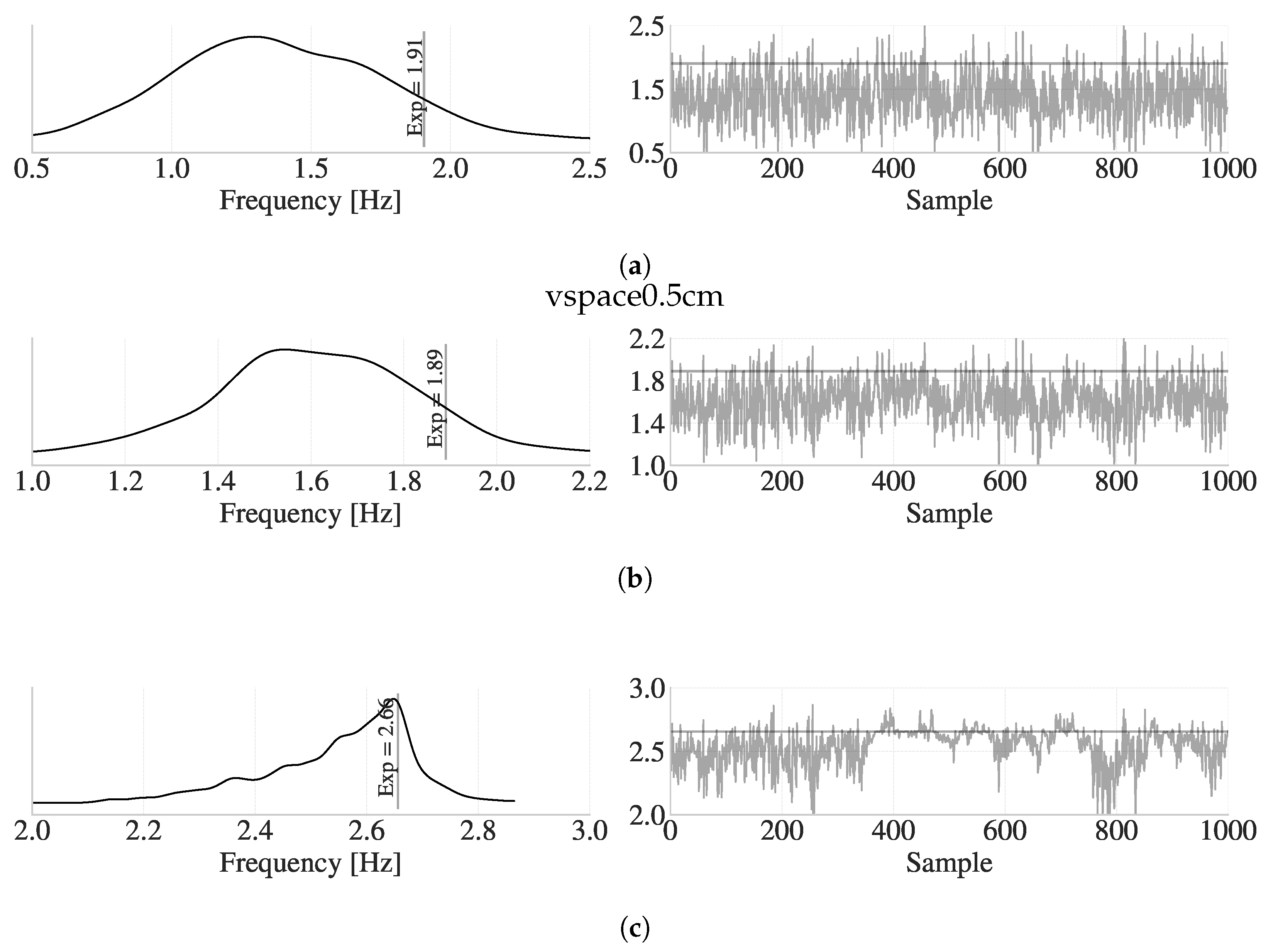
The natural frequencies and damping ratios associated with ten structural mode shapes were identified by Pantoli et al. (2016) [35] using AVT data. Two output-only system identification methods, Data-Driven Stochastic Subspace Identification (SSI-DATA) and Natural Excitation Technique combined with Eigensystem Realization Algorithm (NExT-ERA), were utilized for estimating the modal properties of the building. Both methods assume broad-band and stationary excitation for the AVT data [36]. Among the ten identified mode shapes, the first three modes and associated frequencies from SSI-DATA were selected in this study for the Bayesian updating of the parameters. The identified frequencies for the mode shapes are 1.91 Hz, 1.89 Hz, and 2.66 Hz, corresponding to the first, second, and third modes, respectively. These mode shapes were classified as longitudinal, transverse+torsional, and torsional, respectively.
Astroza et al. (2016) [36] utilized the Modal Assurance Criterion (MAC) value to determine that the identified mode shapes from each method were not significantly different, implying that any alternative method would not have substantially altered the results. The identified modal properties provided crucial input for further model updating and accurate structural assessment of the building.

4. Methodology

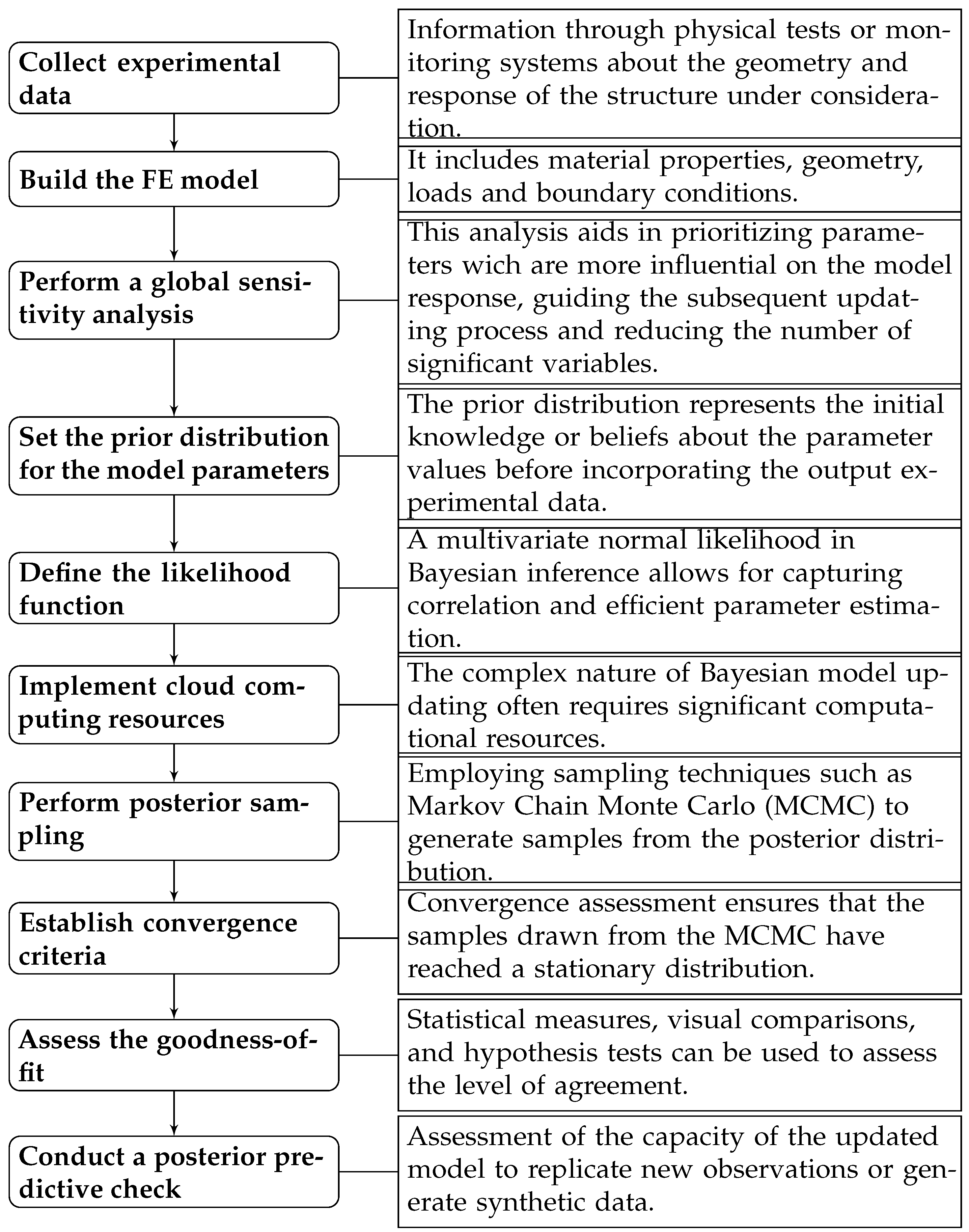
The general methodology for implementing the Bayesian parametric update in the model of the five-story building is illustrated in Figure 2. This diagram provides a comprehensive overview of the steps involved in the methodology, which will be further elaborated upon in the subsequent subsections, with a particular emphasis on the critical steps.

4.1. Modeling of the Structure

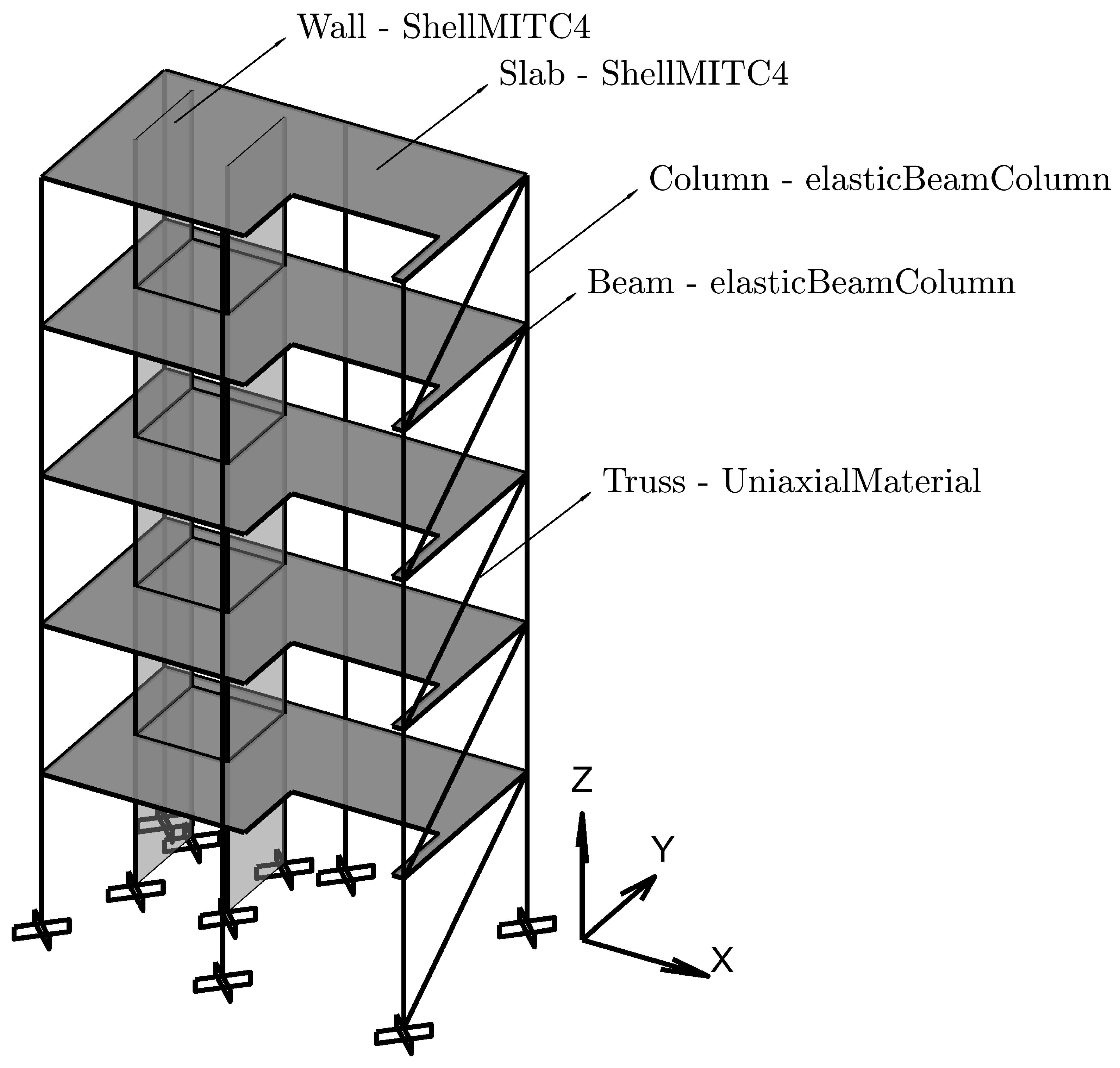
The model presented in this study is built upon the foundation of a previously developed model by Gutierrez (2020) [37]. The building is modeled in Opensees using a FE program in Python called Openseespy. Figure 3 shows a graphical representation of the 3D FE model developed in Openseespy. The structure is first discretized into elements and nodes. Then, the elements’ shape, type, boundary conditions, and dimensions are defined. The model consists of 20 input parameters, such as the moduli of elasticity E for beams, columns, slabs, and walls, and two output parameters, which are the modal coordinates and frequencies of the first three mode shapes. The selection of these parameters is made based on the availability of experimental data during the course of this study. This choice is guided by the aim of utilizing the most pertinent and credible information from the experimental test. Beams and columns are modeled using the elasticBeamColumn element. The ShellMITC4 element is used for slabs and walls, which are joined with approximately 750 nodes. The moduli of elasticity are defined as variable parameters in the model. The beam elements are separated into two groups on each floor: beams on the X-axis and Y-axis. Each group has the same E per level and a cross-sectional area of 0.22 m 2 . The slabs of each floor are discretized into 184 elements, where each shell element has an elastic section with a depth of 0.20 m. The 0.19 m side walls are modeled with 80 shell elements, reaching from the base of the building to the roof. The truss members are modeled with a fixed E using the UniaxialMaterial element, where steel properties are implemented as an elastic material. These truss elements are included in the model as fictitious members with strain-rate effects, making them suitable to include damping in the system [34].
The shear modulus (G) for each of the mentioned structural elements is calculated indirectly using a function that incorporates Poisson’s ratio ( ν ) and the modulus of elasticity (E) (See Equation (6)). The value of ν is set as constant and defined as 0.16 following the work of Pearson (1999) [38].
G = E 2 ( 1 + ν )
A remarkable aspect to consider is that the utilized calibration model may not have fully accounted for the presence of stiff zones in the joints. In practice, joints introduce stiffness to the structural system due to the connections and interactions between elements. However, in the calibration model, these stiffening effects might not have been explicitly included, leading to an underestimation of the overall stiffness.
In order to address the absence of stiff zones in the joints, the calibration process indirectly increased the moduli of elasticity for beams and columns. By raising the moduli of elasticity, the model effectively incorporates the stiffening effects that would be present in the joints, although in an indirect manner.

4.2. Global Sensitivity Analysis

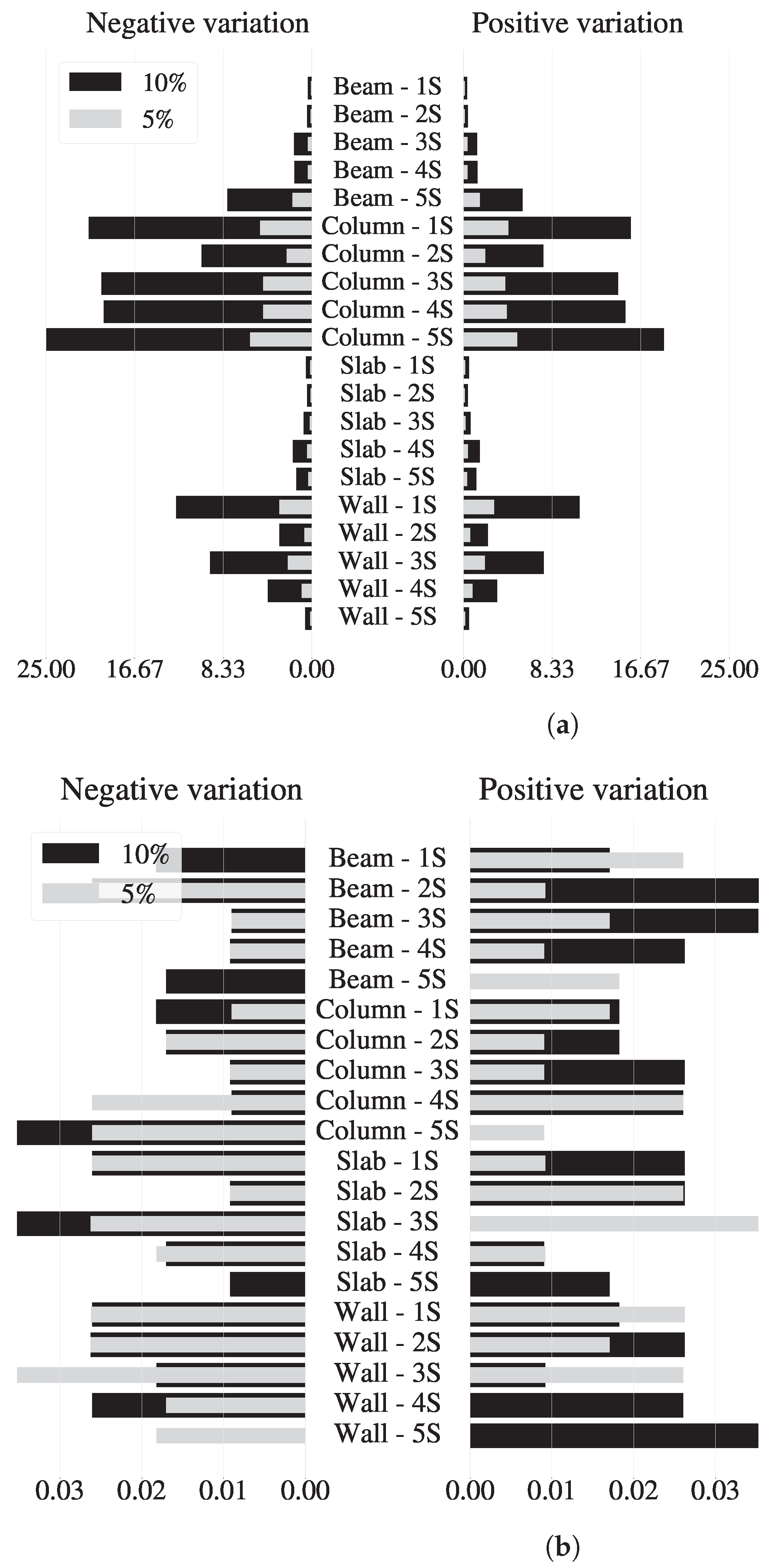
As explained in the previous section, the FE model is defined with 20 input parameters, which are the moduli of elasticity for the structural elements. Before carrying out the updating process, it is important to investigate which parameters have the most significant effects on the response that will be subsequently used for estimation. Thus, a one-at-a-time (OAT) local sensitivity analysis is performed by varying each parameter by ±5% and ±10% of its corresponding nominal value. Then, the variation effects on the model outputs are subsequently studied. The responses obtained by perturbing each model’s parameter (i.e., keeping the others fixed) are compared with the response obtained with the nominal values of each parameter (Figure 4).
Figure 4a shows that the most sensitive parameters for the frequencies correspond to the moduli of elasticity of columns, while the least sensitive parameters correspond to the moduli of elasticity of slabs. However, in the case of mode shapes (Figure 4b), there is no structural element whose modulus of elasticity parameter is particularly sensitive. The values presented in Figure 4a,b are obtained through the calculation of the mean squared error (MSE) using the vector of experimental and model values of the mode shapes and frequencies. By utilizing this approach, we may assess the level of agreement between the experimental and model values, providing a comprehensive evaluation of the accuracy and performance of the model in capturing the experimental data. The sensitivity analysis results only provide information on the relative importance of the model parameters on the building’s first three natural frequencies and mode shapes. However, it does not mean that a higher preponderance is given to some structural elements when performing the model updating. Hence, a direct comparison of the influence of input parameters in the model is feasible, particularly in relation to the moduli of elasticity of specific beams such as the second and third level beams (Beam 3S and Beam 4S, respectively). These beams exhibit a similar influence on both mode shapes and associated frequencies, allowing for a meaningful evaluation of their respective contributions. Although the amplitude of the shape modes does have an influence on the results depicted in Figure 4, it is not the decisive factor in the regrouping of variables. This is primarily due to the error calculation method employed in the analysis. These results define a regrouping of the input parameters to make more efficient use of the available computational resources. The regrouping is performed with the idea that all parameters included in a subgroup have a single associated Probability Density Function (PDF). As shown in Table 2, seven groups are defined and divided based on their PDFs.

4.3. Bayesian Updating Algorithm

4.3.1. Likelihood Function Estimation

As the likelihood function serves as a bridge between prior knowledge and new information, the correct likelihood function depends on the type of data being analyzed and the nature of the estimated parameters. There are various forms that the likelihood function may take, such as normal distributions and gamma distributions, each tailored to a specific problem. The multivariate normal distribution is chosen because it may adequately capture the relationships between multiple observations, making it well-suited for modeling complex systems. The multivariate normal distribution also has well-understood properties for propagation errors and estimating uncertainty, making it a useful tool for Bayesian model updating. Following the definition made in Equation (4), the vectors x and μ are expressed with the following configuration:
μ = f 1 exp f 2 exp f 3 exp Φ 1 , 1 exp Φ 1 , 20 exp Φ 2 , 1 exp Φ 2 , 20 exp Φ 3 , 1 exp Φ 3 , 20 exp 63 × 1 x = f 1 mod f 2 mod f 3 mod Φ 1 , 1 mod Φ 1 , 20 mod Φ 2 , 1 mod Φ 2 , 20 mod Φ 3 , 1 mod Φ 3 , 20 mod 63 × 1
where f i represents the frequency of the mode shape i, while Φ i , j denotes the modal coordinate j of the mode shape i. The subscripts e x p and m o d indicate the experimental and model values, respectively.
The weight matrix W is defined in this study as:
W = 1 0 0 0 0 0 0 0 1 0 0 0 0 0 0 0 1 0 0 0 0 0 0 0 1 20 0 0 0 0 0 0 0 1 20 0 0 0 0 0 0 0 1 20 0 0 0 0 0 0 0 1 20 63 × 63
where the first three values in the diagonal of the matrix contain the weights of the frequency values associated with the first three mode shapes, and the weights of the modal coordinates for the first three modes are in the following 60 values. Since there are 20 modal coordinates for each mode, the respective values are normalized by a factor of 1/20, while the associated frequencies are multiplied by a factor of 1, thus giving each mode the same weight as its corresponding frequency.
Following Equation (5), the covariance matrix measures the degree of interdependence between output variables in a dataset. In the diagonal elements, σ i 2 , with i 3 , corresponds to the variance of the frequency associated with the i mode shape, and i > 3 corresponds to the variance of respective modal coordinates. The off-diagonal elements are the covariance between a pair of output variables, whether frequencies or mode shapes.

4.3.2. Posterior Sampling

The model updating is performed using Python together with the following libraries: Arviz for the exploratory analysis of Bayesian models, Numpy for the implementation of mathematical functions and linear algebra operators, Bilby for parameter estimation using BI [39], Matplotlib for plotting, Scipy as a statistical package (probability distributions, correlation functions, etc.), Emcee as a sampler of Goodman and Weare’s Markov chain affine invariant [40], Pandas for data manipulation and analysis, and Openseespy as Opensees interpreter.
The numerical model updating of the structure aims to estimate the parameter set of the x vector that maximizes the likelihood function ϕ ( x ) (Equation (4)). However, it is necessary to include the MAC to ensure that the correct modal forms are being compared. To ensure that a pair of experimental and model mode shapes are comparable, it is necessary to both normalize the mode shapes and calculate the MAC value between them. Once the MAC value has been calculated, the mode shapes can be compared, and the highest MAC value indicates the most similar mode shapes. The covariance matrix is automatically estimated using the command integrated into the Numpy library.
The numerical model code is included within the main Bayesian updating code to save resources in data transfer in the system to be worked. The estimations are performed using a Markov chain Monte Carlo (MCMC) ensemble sampler with 142,000 samples and LogNormal distributions as priors for all parameters (Table 3). Values for the prior distributions are obtained from the experimental data available in [34]. The choice of using a LogNormal distribution is based on the work conducted by Mirza and MacGregor (1982) [41] and Nowak and Szerszen (2003) [42]. These studies involved collecting a substantial amount of data on the compressive strength of concrete, which is closely associated to the modulus of elasticity. It was observed that the data in both studies exhibited a distribution that could be reasonably approximated by a LogNormal distribution.

4.4. Cloud Computing as Alternative

One of the main drawbacks faced in this study is the execution time of the Bayesian updating algorithm. In this case, two variables have the most significant impact on running time: the quantity of nodes and elements of the FE model and the relatively low sensitivity between the input parameters and the model’s output. Therefore, the Infrastructure-as-a-Service (IaaS) cloud computing provided by Google is used based on its scalable and cost-effective way of using Virtual Machines (VM) on demand, charging them only for the computing resources leased for a period. Moreover, Google cloud service allows integration with Google Colaboratory, an open-source Python programming tool used primarily for machine learning. Natively, Google Colaboratory uses VMs to run the notebook code on the server. The VM used in this study was the c2-standard-8, which focuses on ultra-high performance for processing-intensive workloads and is mainly used for workloads linked to processing. The complete model-updating simulation took about 215 h.

5. Results and Discussions

In this section, it will be presented and compared the results obtained from the two different approaches for the covariance matrix in the likelihood function: calculating the covariance matrix at each iteration and using an identity matrix as the covariance matrix, hereafter, it will be referred to as iterative-approach and identity-approach, respectively.
By comparing the results obtained from these two approaches, it is possible to assess their respective strengths and limitations in terms of accuracy, computational efficiency, and robustness. Such an analysis may help determine which approach is best suited for a particular problem and may inform the design of future studies involving Bayesian updating of structural models.

5.1. Convergence Criteria

The convergence of the Markov chains is verified using two methods: evolution of the Effective Sample Sizes (ESS) and the Markov Chain Standard Error (MCSE). The ESS measures the efficiency of Monte Carlo methods reaching the number of effective samples necessary for estimating the posterior distribution of the corresponding parameter to have enough information to guarantee a satisfactory result according to the evaluator’s criterion [43]. In this case, the limit number that needs to be exceeded to guarantee convergence according to the method is 400 effective samples [44]. For both, iterative-approach and identity-approach, using the bulk-ESS and tail-ESS methods, the number of effective samples obtained in the chain far exceeds the limit, shown in Figure 5, with more than 2000 in the first case and more than 5000 in the second. In most of the chains, the iterative-approach shows a slightly faster convergence compared to the identity-approach. This may be due to the fact that the iterative-approach takes into account the specific characteristics of the data, allowing for a more precise estimation of the posterior distribution. However, the difference in convergence speed between the two approaches is so small that it may be considered negligible.
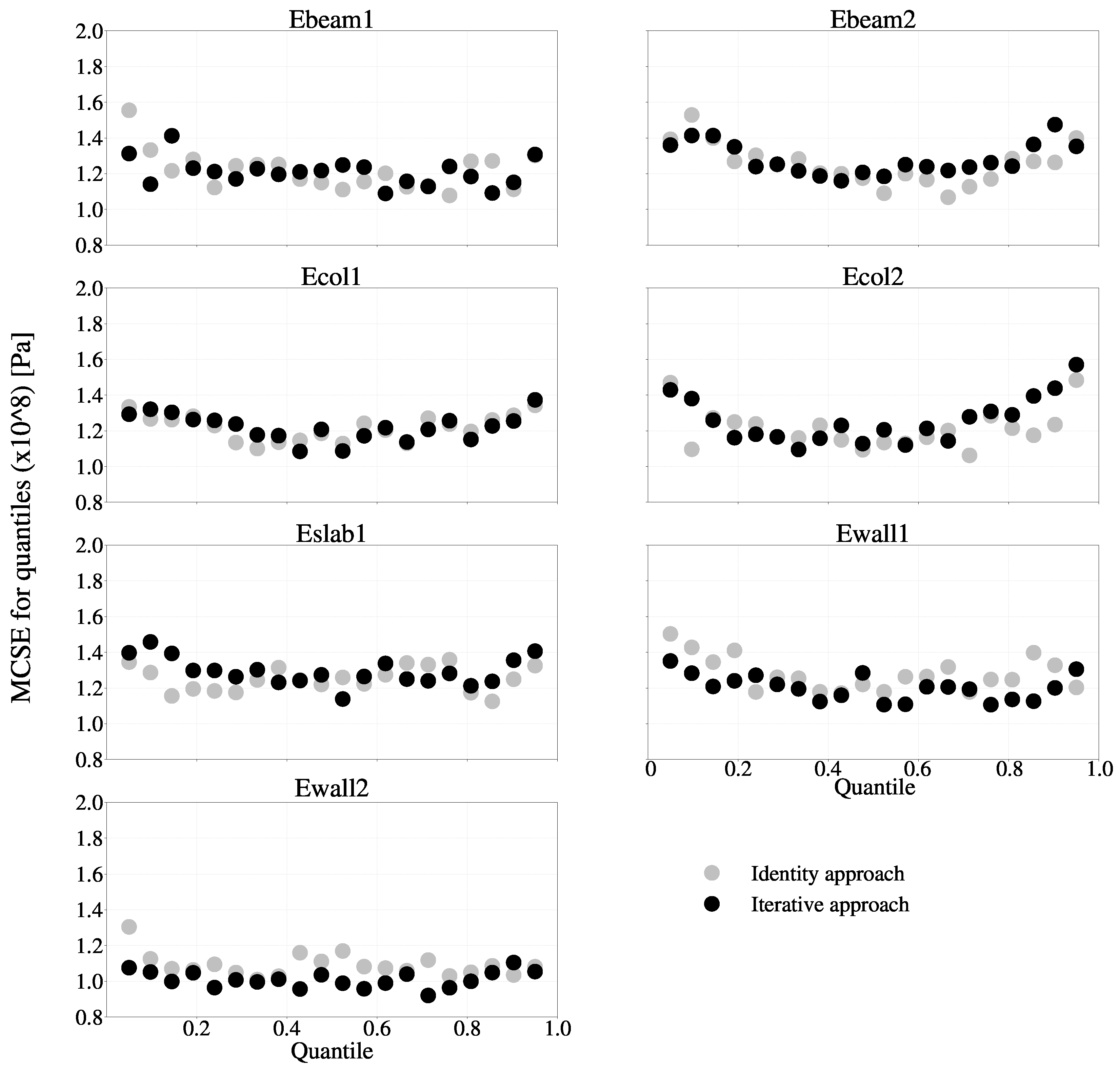
On the other hand, the MCSE method is defined as the standard deviation of the chains divided by their effective sample size [45]. The MCSE provides a quantitative measure of the magnitude of the estimation noise. Although the acceptable limit is also given at the discretion of the researcher, the acceptable uncertainty associated with the mean of the posterior distribution may be taken as a reference (Figure 6). The MCSE results indicate that there is no significant difference in the precision of estimating the posterior distribution of the parameters between the two approaches. Thus, both approaches may be considered equally effective in estimating the posterior distribution.

5.2. Numerical Evaluation of the Model Updating

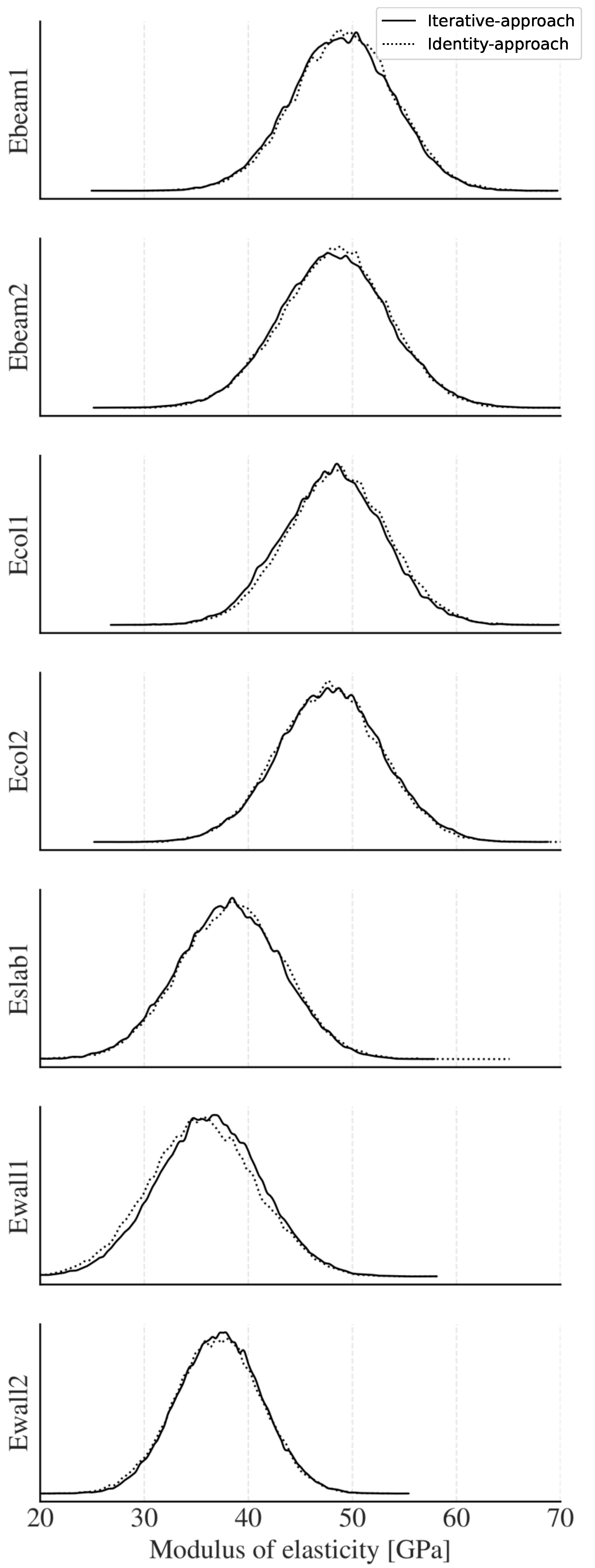
The posterior probability density allows for a detailed analysis of the model parameters, including the identification of the most likely values, the range of uncertainty, and the correlation between different parameters. Thus, Figure 7 illustrates the final distribution obtained for each parameter using both approaches. The figure provides a visual representation of the PDF generated through the respective methods and allows for a comparative analysis of the results.
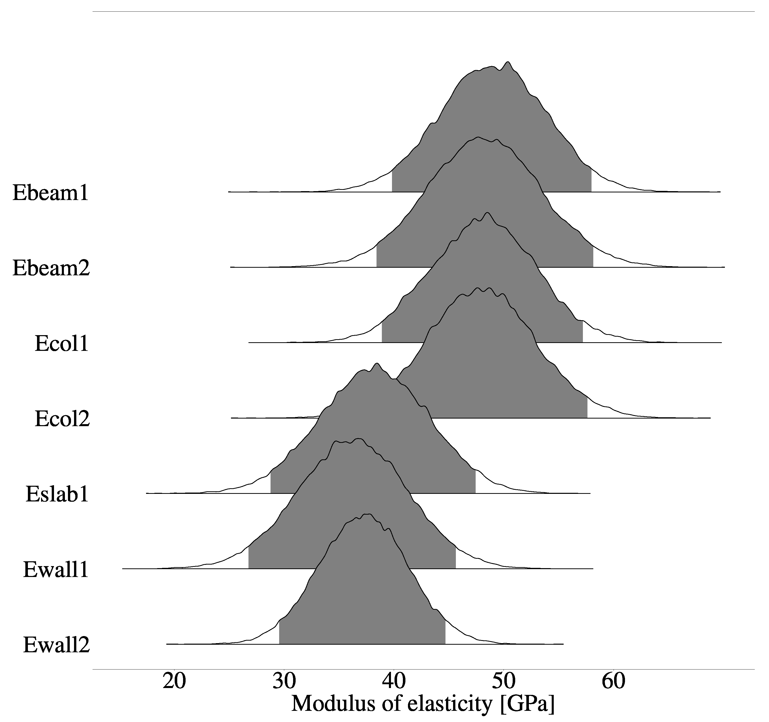
Figure 8 illustrates that the posterior distributions obtained from both approaches exhibit significant overlap, indicating that they are almost identical. It depicts the trends and high-density intervals for each parameter where Ebeam 1 , Ebeam 2 , Ecol 1 , and Ecol 2 have a considerably higher modulus of elasticity than Eslab 1 , Ewall 1 , and Ewall 2 . These plots may effectively highlight data points deviating significantly from the expected trend. The posterior distribution of the model parameters is found to be highly comparable between both approaches, indicating that the precision in estimating posterior distributions is comparable as well. Decision-makers may use this information in designing or assessing engineering models [46].
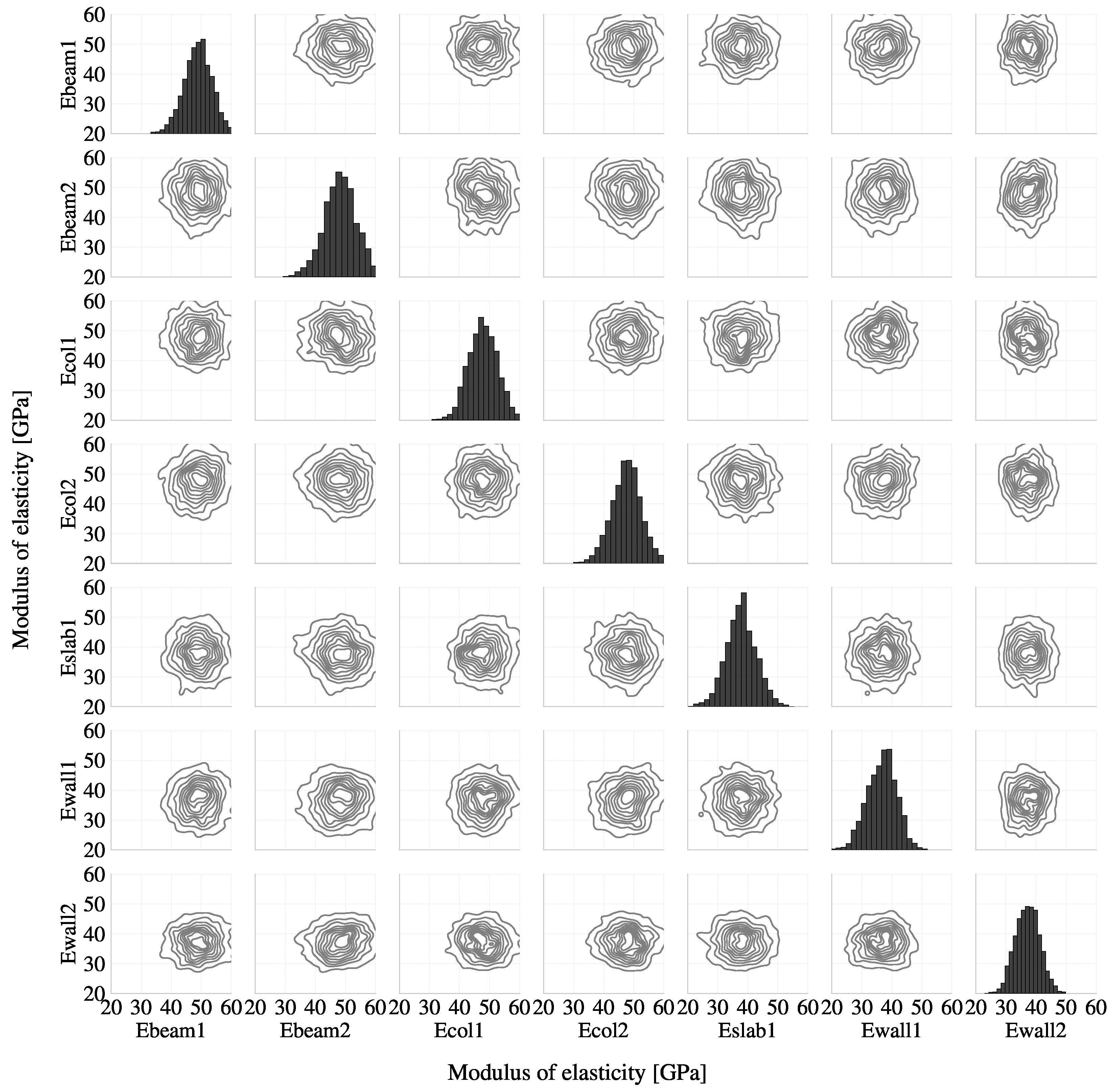
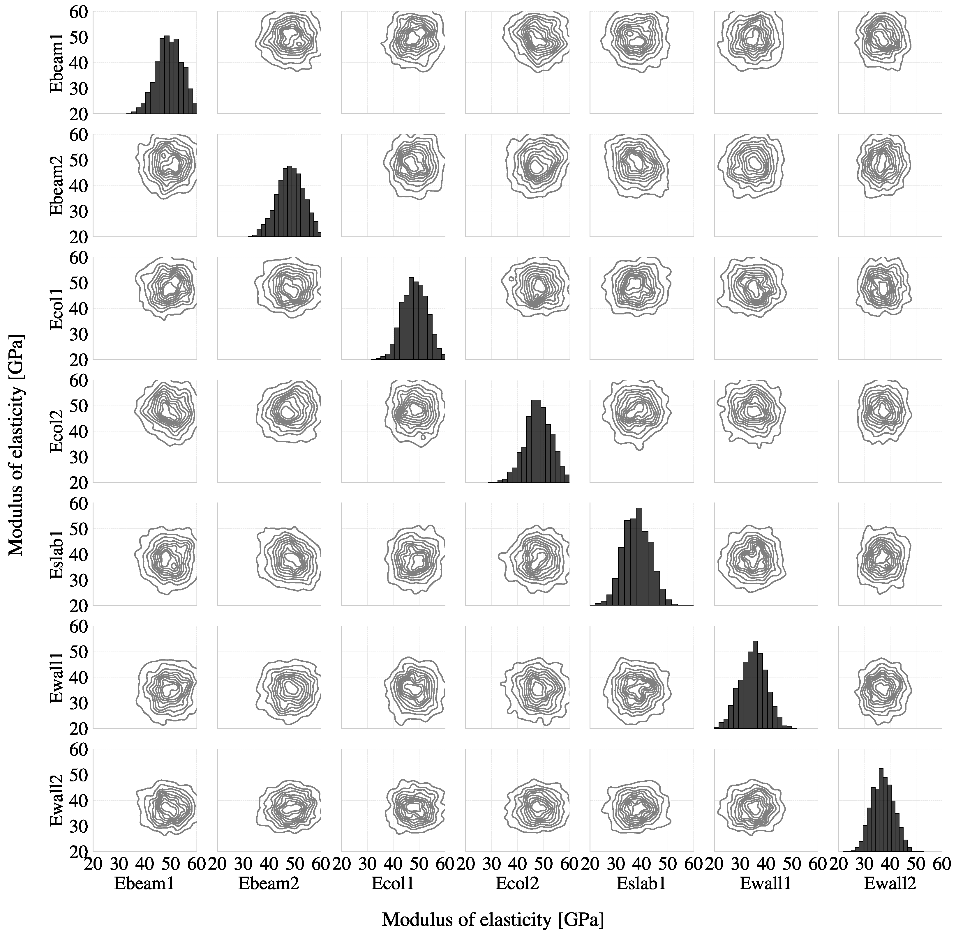
Figure 9 and Figure 10 with their respective Table 4 and Table 5 illustrate the pairwise relationship between model parameters and their corresponding marginal distributions in a corner plot, allowing for a visual interpretation of the parameter correlations and providing insights into the model’s behavior. These figures reveal weak correlations between variables by both approaches, which may be attributed to the inherent independence of input variables in FE models.
Table 6 presents Pearson’s correlation coefficients for the posterior distribution of model parameters obtained from the two approaches: iterative-approach and identity-approach. The above-the-diagonal values represent the correlation coefficient obtained from the iterative-approach and the below-the-diagonal values represent the correlation coefficient obtained from the identity-approach. This table provides valuable information about the correlation between the posterior distribution of model parameters obtained from the two approaches, which may be useful for understanding the impact of the covariance matrix on the estimation of the posterior distribution. The values in bold represent the largest values for a coefficient between the same parameters. As the results are mixed, it is difficult to establish a clear correlation between the parameters and either of the approaches. Initial regrouping of highly correlated parameters performed in Section 4.2 may have contributed to general weak correlations between the model final parameters.
This study uses two key parameters to assess the accuracy of the structural response and the effectiveness of the model updating. First is the Posterior Predictive Check (PPC), which evaluates the agreement between observed and predicted responses. Second is the Modal Assurance Criterion (MAC), which quantifies the similarity between experimental and updated modal properties. Given the similar results obtained from both approaches in the posterior distributions, either approach will be used interchangeably to compute the results derived from the posterior distributions going forward. Figure 11a–c show the results of a subsequent prediction check in which the frequencies predicted by the model are compared with the observed data. A PPC is used to evaluate the goodness-of-fit of the model and the data, involving the generation of new frequency sets based on estimated model parameters and a comparison to the experimental data. It compares the predictions generated by the model with the actual observed values (experimental). Analyzing the PPC plot compared to experimental values helps validate the model’s predictions and provides insights into its performance and reliability. The results present a good model performance relative to the experimental data used in the updating process. Specifically, the model’s predictions closely match the observed data in terms of the frequencies, providing evidence of the model’s improved accuracy and reliability.
The quality of the mode shape comparison is quantified by the MAC values, where a value of 1 indicates a perfect match of the mode shapes between the experimental and FE model. The modal coordinates and associated uncertainties are calibrated using the posterior distribution of the updated model parameters, followed by a comparison of the resulting MAC with experimentally identified data. A graphical comparison of the MAC matrix calculated for the value corresponding to the prior and posterior distribution of the modal coordinates is shown in Figure 12. The prior values correspond to the estimated values for the modal coordinates, which are based exclusively on prior information, and are not yet updated with any new data or information. The posterior values correspond to the posterior distribution of the modal coordinates, which means that the estimated values for the modal coordinates, after the Bayesian updating process, have been incorporated into the analysis. As shown in the diagonal elements of the MAC matrix, the proposed updates have significantly improved the fit of the FE model to the experimental results. The updated MAC values are closer to 1 than the initial values, indicating a closer agreement between the updated model and the experimental measurements. The good performance in the MAC fit suggests that this Bayesian model-updating approach effectively captured the uncertainties and updated the model parameters to match the experimental results.

5.3. Covariance Matrix Analysis

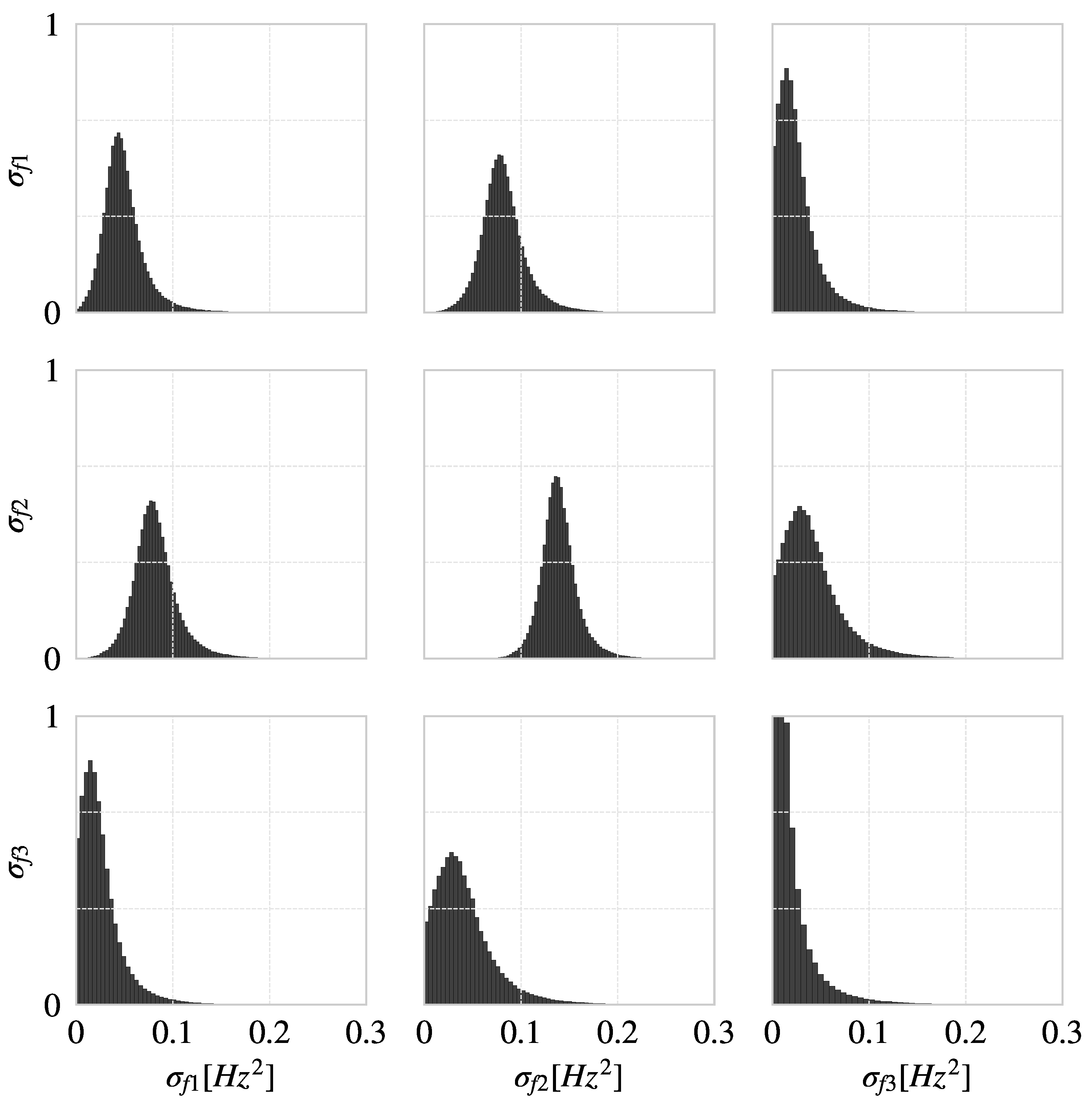
The covariance matrix is a type of matrix that provides insights into the correlation between frequencies and mode shapes and their associated uncertainties [27]. The shape and values of the covariance matrix reveal critical structural features such as the degree of symmetry, the presence of localized modes, and the overall complexity of the vibration patterns. Through a modification in the source code of the BI library, it is possible to save the covariance matrix for each sample. The original matrix has a size of 63 × 63; however, only those corresponding to the first three frequencies are shown in Figure 13. The variance (main diagonal elements) and covariance (off-diagonal elements) of the frequencies are plotted together in this plot. A higher covariance between two natural frequencies indicates a more significant correlation between the corresponding vibration modes of the structure.

6. Conclusions

This paper implemented a methodology for updating the structural model parameters using BI. The modal properties of a five-story full-scale RC building were used to update the FE model. The parametric uncertainty quantification process and its results were explained following the proposed methodology. The updating algorithm determined the posterior probability of the FE model’s parameters and calculated the covariance matrix of the observations, comparing them with model realizations. The covariance matrix between observations and the updated model allowed for identifying the error computed through a multivariate normal likelihood function.
Although, in theory, iteratively calculating the covariance matrix enabled a more comprehensive understanding of the system’s behavior, both used approaches for incorporating the covariance matrix into the Bayesian model-updating framework (identity-approach and iterative-approach) resulted in similar posterior distributions and convergence rates. Therefore, in this case, both approaches may be used interchangeably without affecting the results’ reliability or accuracy. This finding provides a practical advantage in terms of computational efficiency when dealing with large sample sizes.
The obtained posterior updating of the input parameters of the FE model corresponds to distributions similar to normal shapes without clear biases, i.e., approximately symmetric distributions. In all cases, the posterior distributions have a smaller standard deviation with respect to the prior distributions. Therefore, the error associated with the model and parameter’s values is smaller than initially assumed. Furthermore, the way the MAC function was calculated provides valuable information about the reliability of the model update in terms of mode shapes, highlighting the importance of quantifying the uncertainty associated also with the associated frequency through PPC and its comparison with experimental data. The proposed methodology may improve the reliability of structural models and assist in decision-making for the design and assessment of structures.

Author Contributions

Conceptualization, O.D.H., A.R.O., D.G. and R.A.; methodology, O.D.H. and A.R.O.; formal analysis, O.D.H. and A.R.O.; funding acquisition, A.R.O. and D.G.; writing—original draft preparation, O.D.H.; writing—review and editing, D.G., A.R.O. and R.A. All authors have read and agreed to the published version of the manuscript.

Funding

This work was financially supported by the Universidad del Valle, Colombia (Grant No. 21185: Evaluation of structural reliability reliability of reinforced concrete elements subjected to reinforced concrete elements subjected to flexural and shear).

Acknowledgments

The authors would like to acknowledge Matthew Pitkin from University of Glasgow (Scotland) for providing suggestions in the model-updating algorithm and Mathias Gutiérrez from Universidad de los Andes (Chile) for providing information about the numerical model of the structure.

Conflicts of Interest

The authors declare no conflict of interest.

References

  1. Armstrong, C.G. Modelling requirements for finite-element analysis. Comput.-Aided Des. 1994, 26, 573–578. [Google Scholar] [CrossRef]
  2. Shan, S.; Wang, G.G. Survey of modeling and optimization strategies to solve high-dimensional design problems with computationally-expensive black-box functions. Struct. Multidiscip. Optim. 2010, 41, 219–241. [Google Scholar] [CrossRef]
  3. Zárate, B.A.; Caicedo, J.M. Finite element model updating: Multiple alternatives. Eng. Struct. 2008, 30, 3724–3730. [Google Scholar] [CrossRef]
  4. Jagota, V.; Sethi, A.P.S.; Kumar, K. Finite element method: An overview. Walailak J. Sci. Technol. (WJST) 2013, 10, 1–8. [Google Scholar]
  5. Rios, J.M. Uncertainty in Structural Dynamic Models. Ph.D. Thesis, Swansea University, Swansea, UK, 2005. [Google Scholar]
  6. Igusa, T.; Buonopane, S.; Ellingwood, B. Bayesian analysis of uncertainty for structural engineering applications. Struct. Saf. 2002, 24, 165–186. [Google Scholar] [CrossRef]
  7. Bulleit, W.M. Uncertainty in structural engineering. Pract. Period. Struct. Des. Constr. 2008, 13, 24–30. [Google Scholar] [CrossRef]
  8. Gomez, D.; Dyke, S.J.; Rietdyk, S. Structured uncertainty for a pedestrian-structure interaction model. J. Sound Vib. 2020, 474, 115237. [Google Scholar] [CrossRef]
  9. Vailati, M.; Monti, G.; Khazna, M.; Realfonzo, R.; De Iuliis, M. Probabilistic seismic response analysis of existing masonry structures. In Brick and Block Masonry; CRC Press: Boca Raton, FL, USA, 2016; pp. 2489–2498. [Google Scholar] [CrossRef]
  10. Zellner, A. Bayesian and non-Bayesian approaches to statistical inference and decision-making. J. Comput. Appl. Math. 1995, 64, 3–10. [Google Scholar] [CrossRef] [Green Version]
  11. Briggs, A.H.; Weinstein, M.C.; Fenwick, E.A.; Karnon, J.; Sculpher, M.J.; Paltiel, A.D. Model parameter estimation and uncertainty analysis: A report of the ISPOR-SMDM Modeling Good Research Practices Task Force Working Group-6. Med. Decis. Mak. 2012, 32, 722–732. [Google Scholar] [CrossRef] [PubMed]
  12. Hoang, T.V.; Matthies, H.G. An efficient computational method for parameter identification in the context of random set theory via Bayesian inversion. Int. J. Uncertain. Quantif. 2021, 11, 1–18. [Google Scholar] [CrossRef]
  13. Sehgal, S.; Kumar, H. Structural dynamic model updating techniques: A state of the art review. Arch. Comput. Methods Eng. 2016, 23, 515–533. [Google Scholar] [CrossRef]
  14. Loyola, M. Big data in building design: A review. J. Inf. Technol. Constr. 2018, 23, 259–284. [Google Scholar]
  15. Beck, J.L.; Katafygiotis, L.S. Updating models and their uncertainties. I: Bayesian statistical framework. J. Eng. Mech.-Proc. ASCE 1998, 124, 455–462. [Google Scholar] [CrossRef]
  16. Katafygiotis, L.S.; Beck, J.L. Updating models and their uncertainties. II: Model identifiability. J. Eng. Mech. 1998, 124, 463–467. [Google Scholar] [CrossRef]
  17. Jaynes, E.T. Probability Theory: The Logic of Science; Cambridge University Press: Cambridge, UK, 2003. [Google Scholar]
  18. Bayes, T. LII. An essay towards solving a problem in the doctrine of chances. By the late Rev. Mr. Bayes, FRS communicated by Mr. Price, in a letter to John Canton, AMFR S. In Philosophical Transactions of the Royal Society of London; Royal Society of London: London, UK, 1763; pp. 370–418. [Google Scholar]
  19. Swinburne, R. Bayes’ Theorem. Mind 2004, 113, 591–596. [Google Scholar] [CrossRef]
  20. Denison, D.G.; Holmes, C.C.; Mallick, B.K.; Smith, A.F. Bayesian Methods for Nonlinear Classification and Regression; John Wiley & Sons: Hoboken, NJ, USA, 2002; Volume 386. [Google Scholar]
  21. MacLehose, R.F.; Hamra, G.B. Applications of Bayesian methods to epidemiologic research. Curr. Epidemiol. Rep. 2014, 1, 103–109. [Google Scholar] [CrossRef] [Green Version]
  22. Ma, Z.; Chen, G. Bayesian methods for dealing with missing data problems. J. Korean Stat. Soc. 2018, 47, 297–313. [Google Scholar] [CrossRef]
  23. Zhang, Z.; Sun, C.; Guo, B. Transfer-learning guided Bayesian model updating for damage identification considering modeling uncertainty. Mech. Syst. Signal Process. 2022, 166, 108426. [Google Scholar] [CrossRef]
  24. Zhang, E.; Feissel, P.; Antoni, J. A comprehensive Bayesian approach for model updating and quantification of modeling errors. Probabilistic Eng. Mech. 2011, 26, 550–560. [Google Scholar] [CrossRef]
  25. Argyris, C.; Papadimitriou, C.; Panetsos, P.; Tsopelas, P. Bayesian model-updating using features of modal data: Application to the metsovo bridge. J. Sens. Actuator Netw. 2020, 9, 27. [Google Scholar] [CrossRef]
  26. Ghurye, S.; Olkin, I. A characterization of the multivariate normal distribution. Ann. Math. Stat. 1962, 33, 533–541. [Google Scholar] [CrossRef]
  27. Tong, Y.L. The Multivariate Normal Distribution; Springer Science & Business Media: Berlin/Heidelberg, Germany, 2012. [Google Scholar]
  28. Srivastava, M.S. Some tests concerning the covariance matrix in high dimensional data. J. Jpn. Stat. Soc. 2005, 35, 251–272. [Google Scholar] [CrossRef] [Green Version]
  29. Srivastava, M.S.; Kollo, T.; von Rosen, D. Some tests for the covariance matrix with fewer observations than the dimension under non-normality. J. Multivar. Anal. 2011, 102, 1090–1103. [Google Scholar] [CrossRef] [Green Version]
  30. Birke, M.; Dette, H. A note on testing the covariance matrix for large dimension. Stat. Probab. Lett. 2005, 74, 281–289. [Google Scholar] [CrossRef] [Green Version]
  31. Fisher, T.J. On testing for an identity covariance matrix when the dimensionality equals or exceeds the sample size. J. Stat. Plan. Inference 2012, 142, 312–326. [Google Scholar] [CrossRef]
  32. Yan, W.J.; Katafygiotis, L.S. A novel Bayesian approach for structural model updating utilizing statistical modal information from multiple setups. Struct. Saf. 2015, 52, 260–271. [Google Scholar] [CrossRef]
  33. Zhang, X.; Boscardin, W.J.; Belin, T.R. Sampling correlation matrices in Bayesian models with correlated latent variables. J. Comput. Graph. Stat. 2006, 15, 880–896. [Google Scholar] [CrossRef]
  34. Chen, M.C.; Pantoli, E.; Wang, X.; Astroza, R.; Ebrahimian, H.; Hutchinson, T.C.; Conte, J.P.; Restrepo, J.I.; Marin, C.; Walsh, K.D.; et al. Full-scale structural and nonstructural building system performance during earthquakes: Part I–specimen description, test protocol, and structural response. Earthq. Spectra 2016, 32, 737–770. [Google Scholar] [CrossRef]
  35. Pantoli, E.; Chen, M.C.; Hutchinson, T.C.; Astroza, R.; Conte, J.P.; Ebrahimian, H.; Restrepo, J.I.; Wang, X. Landmark data set from the building nonstructural components and systems (BNCS) project. Earthq. Spectra 2016, 32, 1239–1259. [Google Scholar] [CrossRef]
  36. Astroza, R.; Ebrahimian, H.; Conte, J.P.; Restrepo, J.I.; Hutchinson, T.C. Influence of the construction process and nonstructural components on the modal properties of a five-story building. Earthq. Eng. Struct. Dyn. 2016, 45, 1063–1084. [Google Scholar] [CrossRef]
  37. Gutierrez, M. Bayesian Finite Element Model Parameter and Covariance Estimation. Master’s Thesis, Universidad de los Andes, Santiago, Chile, 2020. [Google Scholar]
  38. Persson, B. Poisson’s ratio of high-performance concrete. Cem. Concr. Res. 1999, 29, 1647–1653. [Google Scholar] [CrossRef]
  39. Ashton, G.; Hübner, M.; Lasky, P.D.; Talbot, C.; Ackley, K.; Biscoveanu, S.; Chu, Q.; Divakarla, A.; Easter, P.J.; Goncharov, B.; et al. BILBY: A user-friendly Bayesian inference library for gravitational-wave astronomy. Astrophys. J. Suppl. Ser. 2019, 241, 27. [Google Scholar] [CrossRef] [Green Version]
  40. Goodman, J.; Weare, J. Ensemble samplers with affine invariance. Commun. Appl. Math. Comput. Sci. 2010, 5, 65–80. [Google Scholar] [CrossRef]
  41. Mirza, S.A.; MacGregor, J.G. Probabilistic study of strength of reinforced concrete members. Can. J. Civil Eng. 1982, 9, 431–448. [Google Scholar] [CrossRef]
  42. Nowak, A.S.; Szerszen, M.M. Calibration of design code for buildings (ACI 318): Part 1—Statistical models for resistance. Struct. J. 2003, 100, 377–382. [Google Scholar] [CrossRef]
  43. Pinto, F.; Toledo, J.; Birrell, M.; Bazaez, R.; Hernandez, F.R.A. Uncertainty Quantification in Constitutive Models of Highway Bridge Components: Seismic Bars and Elastomeric Bearings. Materials 2023, 16, 1792. [Google Scholar] [CrossRef] [PubMed]
  44. Vehtari, A.; Gelman, A.; Simpson, D.; Carpenter, B.; Bürkner, P.C. Rank-normalization, folding, and localization: An improved for assessing convergence of MCMC (with Discussion). Bayesian Anal. 2021, 16, 667–718. [Google Scholar] [CrossRef]
  45. Kruschke, J. Doing Bayesian Data Analysis: A Tutorial with R, JAGS, and Stan; Academic Press: Waltham, MA, USA, 2014. [Google Scholar] [CrossRef]
  46. Kampenes, V.B.; Dybå, T.; Hannay, J.E.; Sjøberg, D.I. A systematic review of effect size in software engineering experiments. Inf. Softw. Technol. 2007, 49, 1073–1086. [Google Scholar] [CrossRef] [Green Version]
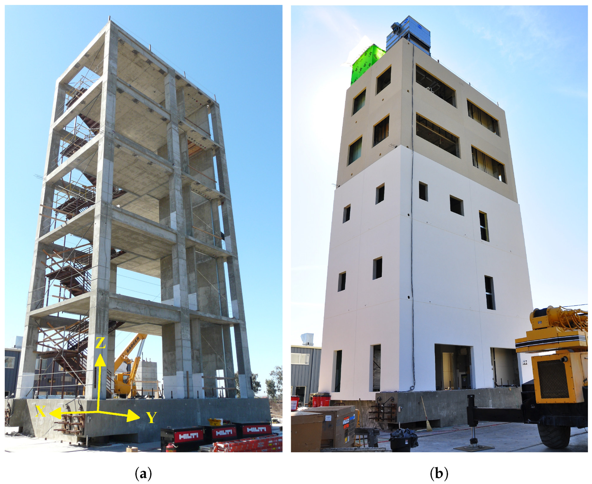
Figure 1. Five-story test building. (a) Bare structure without non-structural elements, (b) Complete structure.
Buildings 13 01568 g001
Figure 2. Workflow of the implemented methodology for Bayesian parametric update in the model of the five-story building.
Buildings 13 01568 g002
Figure 3. Finite element model developed in Openseespy.
Buildings 13 01568 g003
Figure 4. Results of the OAT sensitivity analysis. Note that the number accompanying the letter S indicates the story where the structural elements are. (a) Changes (%) on natural frequencies regarding variations on the moduli of elasticity, (b) Changes (%) on mode shapes regarding variations on the moduli of elasticity.
Buildings 13 01568 g004
Figure 5. Evolution of effective sample size (ESS) for posterior sampling.
Buildings 13 01568 g005
Figure 6. Markov chain standard error (MCSE) for posterior sampling.
Buildings 13 01568 g006
Figure 7. Posterior probability density function and tracing values.
Buildings 13 01568 g007
Figure 8. Posterior probability density function in forest plot. Gray zone: 94.0% HDI. Iterative-approach.
Buildings 13 01568 g008
Figure 9. Corner plot of model parameters. Iterative-approach.
Buildings 13 01568 g009
Figure 10. Corner plot of model parameters. Identity-approach.
Buildings 13 01568 g010
Figure 11. Posterior predictive check and tracing values. (a) Frequency 1, (b) Frequency 2, (c) Frequency 3.
Buildings 13 01568 g011
Figure 12. Prior and posterior MAC PDF.
Buildings 13 01568 g012
Figure 13. First three rows and columns on the Covariance matrix representing the first three frequencies of the building.
Buildings 13 01568 g013
Table 1. Summary results for compressive concrete cylinder tests before seismic testing.
ElementAverage f c [MPa]Average E c [GPa]
Columns and walls57.232.6
Slabs and beams51.733.1
Table 2. Parameter regrouping for Bayesian updating of the structural model.
GroupElementPrevious NomenclatureNew Nomenclature
1Beam—1st StoryEbeam1Ebeam1
Beam—2nd StoryEbeam2
2Beam—3rd StoryEbeam3Ebeam2
Beam—4th StoryEbeam4
Beam—5th StoryEbeam5
3Column—1st StoryEcol1Ecol1
Column—2nd StoryEcol2
4Column—3rd StoryEcol3Ecol2
Column—4th StoryEcol4
Column—5th StoryEcol5
5Slab—1st StoryEslab1Eslab1
Slab—2nd StoryEslab2
Slab—3rd StoryEslab3
Slab—4th StoryEslab4
Slab—5th StoryEslab5
6Wall—1st StoryEwall1Ewall1
Wall—2nd StoryEwall2
7Wall—3rd StoryEwall3Ewall2
Wall—4th StoryEwall4
Wall—5th StoryEwall5
Table 3. Prior distributions for model updating.
Prior Distributions
ParametersType of DistributionMean [MPa]Std. Dev. [MPa]
Ebeam1LogNormal35,0009700
Ebeam2LogNormal35,0009700
Ecol1LogNormal35,0009700
Ecol2LogNormal35,0009700
Eslab1LogNormal35,0009700
Ewall1LogNormal35,0009700
Ewall2LogNormal35,0009700
Table 4. Summary of posterior distribution of model parameters. Iterative-approach.
Mean [GPa]SD [GPa]HDI 3% [GPa]HDI 97% [GPa]
Ebeam148.934.8739.7557.99
Ebeam248.165.2738.3958.18
Ecol148.144.8838.9057.23
Ecol247.925.0338.6057.68
Eslab138.195.0028.7547.48
Ewall136.235.0326.7445.66
Ewall237.254.0529.5044.72
Table 5. Summary of posterior distribution of model parameters. Identity-approach.
Mean [GPa]SD [GPa]HDI 3% [GPa]HDI 97% [GPa]
Ebeam149.224.8640.0158.25
Ebeam248.295.1538.4357.79
Ecol148.554.8539.2857.54
Ecol247.764.9638.5957.25
Eslab138.385.0428.6347.50
Ewall135.555.1725.8445.34
Ewall237.084.1529.2044.77
Table 6. Pearson’s Correlation Coefficient for posterior distribution of model parameters. Above the diagonal: Iterative-approach. Below the diagonal: Identity-approach.
Ebeam1Ebeam2Ecol1Ecol2Eslab1Ewall1Ewall2
Ebeam11−0.016290.010.020.0006330.0099280.007501
Ebeam2−0.00053810.016919−0.003235−0.0059690.008270.004841
Ecol10.0206620.0057841−0.0029670.020706−0.0077230.021349
Ecol20.0191760.012743−0.00739710.006645−0.001015−0.01976
Eslab10.008815−0.023660.0171390.03448910.0129890.010983
Ewall1−0.0033820.0067590.0264540.0050820.02253610.017236
Ewall2−0.0045930.0033770.0241540.010754−0.00095−0.0118941
Disclaimer/Publisher’s Note: The statements, opinions and data contained in all publications are solely those of the individual author(s) and contributor(s) and not of MDPI and/or the editor(s). MDPI and/or the editor(s) disclaim responsibility for any injury to people or property resulting from any ideas, methods, instructions or products referred to in the content.