Uncovering the Efficiency and Performance of Ground-Source Heat Pumps in Cold Regions: A Case Study of a Public Building in Northern China

Abstract

In cold regions, due o the impact of climatic conditions, the heat load in winter and the cooling load in summer are unbalanced. In the long-term operation of the ground-source heat pump (GSHP), the soil heat imbalance phenomenon has still not been successfully solved. Therefore, this study took the GSHP of a public building in the cold area of northern China as the research object. Based on the unit performance data of the system over 8 years and the measured data of the soil temperature field, the long-term operation efficiency of the GSHP in the cold region and the variation law of the soil temperature field were explored. In order to further study the problem of soil heat imbalance, the effect of heat exchange hole groups at different intervals on the underground soil thermal environment after 30 years of operation in the system was simulated, and the optimization scheme of heat exchange hole spacing was proposed. The research results support the improvement and optimization of GSHP design and construction, and have important practical significance for the popularization of GSHPs in cold regions.

1. Introduction

In September 2020, China officially put forward the strategic goals of reaching a carbon peak by 2030 and carbon neutrality by 2060, and the implementation of the double carbon goal has become a national strategy for China’s economic and social development [1]. The Party’s 20 major reports proposed to actively yet prudently promote carbon neutralization, based on China’s energy and resource endowments, adhere to the principle of establishing a carbon peak before breaking it, carry out the carbon peak action step by step in a planned way, and further promote the energy revolution. Adjusting China’s coal-based energy structure, basing itself on its energy and resource endowment, focusing on developing carbon-free and low-carbon new energy, and realizing energy independence will be important strategic measures for China in its second 100-year journey.

As a new energy source with rich resources, clean and environmental protection, and high efficiency and stability, the ground-source heat pump has rapidly developed as an alternative form of energy, especially for winter heating in cold areas of northern China [2]. China has applied the GSHP for heating purposes for more than 40 years [3]. According to the China Energy Development Report, the area of the GSHP for building heating reached 1.6 billion square meters in 2020. In the early stage of ground-source heat pump application, people were troubled by the initial investment and operational reliability of the system. With the popularization of the application of this technology and the continuous improvement of the equipment localization rate, the problem of high initial investment in the system has been gradually solved, and people are now more concerned about the long-term operation and reliability of the system.

The soil temperature field is considered to be integral to the operational stability of the large-scale GSHP. Large-scale GSHPs require hundreds of heat exchange holes for heat exchange, and, after long-term operation, thermal interference phenomena exist between the heat exchange holes, leading to changes in the underground thermal environment and affecting the efficiency of GSHPs [4]. Meanwhile, in actual use, the installation of heat exchange holes takes up a lot of space, which also limits the promotion of GSHP technology [5]. In northern Canada, where energy demand in most buildings is dominated by heating, the heating and cooling loads are unbalanced, resulting in lower soil temperatures after long-term operation, affecting system performance factors and ecology [6]. Therefore, it is important to grasp the changes in the heat exchange hole spacing and soil thermal environment of large-scale GSHPs in long-term operation to ensure the safe and efficient operation of the system.

Koohi-Fayegh et al. [7] simulated the two-dimensional transient heat transfer in the soil around two adjacent boreholes and showed that the distance between boreholes directly affects the heat transfer of the system. Yan Y et al. [8] grouped GHEs into squares and classified them into the three types of side, center, and corner holes, according to their locations, which can be used to evaluate the thermal performance of boreholes with different spacing ratios and spacing distances. The results show that increasing either the spacing ratio or the spacing distance can improve the heat transfer for the same running time, while increasing the spacing distance has less effect on the heat flux at a certain spacing ratio. Mustafa Inallf et al. [9] verified the effects of the depth of heat exchanger arrangement, as well as the quality and flow of antifreeze on the performance of the shallow GSHP, by experiments. The experimental data show that the average performance coefficients of SPF are 2.66 and 2.81, respectively, for horizontal buried pipe systems with different trenches at depths of 1 m and 2 m. The experimental results show that the GSHP is suitable for measuring climatic conditions in Turkey [10].

GSHPs started being used in China in the 1980s, and the number of buildings using GSHPs increased rapidly in the following years. Zhi. J.L et al. [11] simulated the variation in soil temperature during GSHP operation in three cities in the cold regions of China to demonstrate the stability of the system over 10 years of operation. You T et al. [12] pointed out the main causes of soil thermal imbalance, including lower soil temperature, lower system performance, lower reliability, and system failure. As an important factor restricting the development of GSHPs in severe cold areas, the imbalance of soil heat intake and release directly leads to a decrease in soil temperature. Qian and Wang [13] have simulated the heat balance of GSHPs in four different working conditions in the heating season and the cooling season. The heat pump only ran in the summer when the cooling load was 50 kW. After 10 years of long-term operation, the soil temperature changed from 17.5 °C to 39.1 °C. The heat pump only ran with a heat load of 50 kW in winter, after 10 years of the long-term operation of the system, and the soil temperature gradually decreased from 17.5 °C to 6.9 °C. Yu and Liu [14] measured soil temperature changes in a residential building in Beijing during the GSHP’s 10-year operation, and found that the soil temperature changed and the temperature difference decreased by 3 °C under the condition of seasonal load balance between winter and summer. Under the condition that the intermittent operation of the system in summer led to the imbalance of seasonal load in winter and summer, the soil temperature decreased by about 4.5 °C. You and Wang [15] took the three cities of Shenyang, Changchun, and Harbin as examples to simulate that after 10 years of GSHPs operating without heat compensation, the soil temperature decreased by 10.9 °C, 11.7 °C, and 11.6 °C, respectively. After using the heat-compensated GSHP, the soil temperature remained stable, effectively solving the problem of soil temperature imbalance. Shang et al. [16] observed that due to the decrease in soil temperature, the heat exchange rate and the heat pump COP both significantly decreased, and the compressor power increased. After 12 h of operation, the COP decreased about 0.6~0.8. Liu et al. [11] analyzed a GSHP system in a cold area, with annual heating and cooling loads of 818,228 kW/ h and 192,351 kW/ h, respectively. Soil temperature and borehole inlet and outlet temperatures showed a decreasing trend over the last 10 years. In the second year, the COP of system efficiency decreased dramatically due to the borehole medium (such as water or refrigerant) temperature below 0 °C.

Studies have found that the performance of the buried pipe heat exchanger has a great impact on the GSHP and soil heat balance, and a good borehole layout is very important for soil temperature recovery, which is closely related to the contact area of the surrounding soil and the appropriate distance between the buried pipes. Retkowski et al. [17] simulated the GSHP system and analyzed the average soil temperature changes at three different distances. The results show that the temperature drop near the borehole was more serious. The maximum temperature drop after 25 years was 12 °C. Gultekin et al. [18] simulated and studied the effect of heat exchange hole spacing on heat transfer efficiency. The different heat exchange hole distances were studied and the best distance was determined. However, increasing the distance between buried pipes will increase the land area and lead to an increase in the initial investment of the project, which is difficult to achieve in densely populated cities.

Due to the short history of large-scale soil source heating engineering applications in China, previous research work has deeply discussed the short-term operation data and simulated operation of the system, and there are few studies on the measured data of long-term system operations, and an even less comprehensive analysis of changes in the underground thermal environment. For the long-term operation of GSHPs in cold regions, in particular, the phenomenon of soil thermal imbalance has not been successfully solved. This paper selects a GSHP in a public building that has been in operation for 8 years. The project is located in Changchun, a cold region of China. The building is a demonstration project of the National Twelfth Five-Year Plan research project. In order to monitor the operation of the GSHP in real time and study the changes in the soil temperature at different underground depths, a monitoring GSHP platform and a soil temperature monitoring well with a depth of 100 m were designed before the project was implemented. Combined with the monitoring platform, the monitoring data of unit performance and underground soil temperature were studied and analyzed. Meanwhile, CFD software was used to simulate the effect of the heat exchanger hole on the underground soil temperature under different spacing conditions after the system has been in operation for 30 years, and an optimization scheme for the spacing of heat exchanger holes in cold regions was proposed. This study provides the first-hand real-time monitoring data of the operation of GSHPs in cold regions, as well as the temperature field change data of different depths of underground soil for 8 consecutive years.

2. System Profile

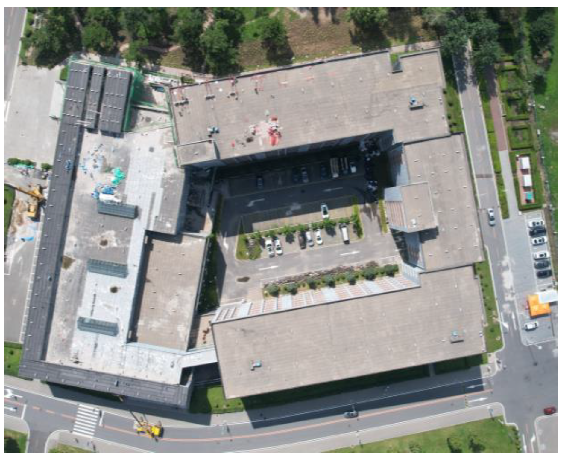
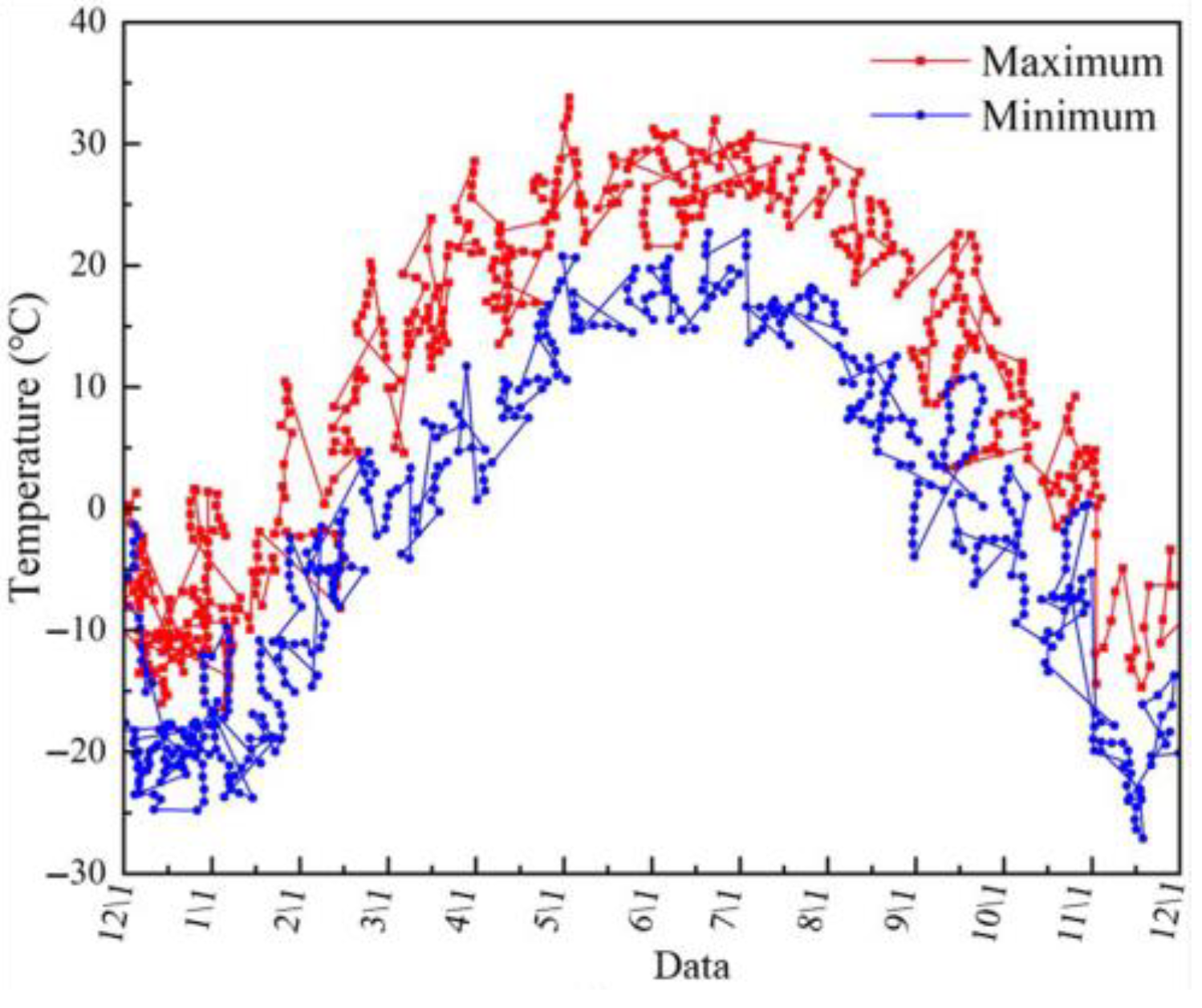
2.1. Project Overview

Figure 1 shows the aerial view of public buildings in Changchun, China. Located in a cold region, Changchun belongs to the temperate continental subhumid monsoon climate type. Winters are severe and long, springs are dry and windy, summers are warm and short, and autumns are sunny with large temperature differences. The average annual temperature is 4.8 °C, the average temperature of the hottest month (July) is 23 °C, the highest temperature is 39.5 °C and the lowest temperature is −39.8 °C. The average annual precipitation is 522~615 mm, with summer precipitation accounting for more than 60% of the annual precipitation [19]. The annual outdoor temperature change curve is shown in Figure 2. The meteorological parameters of HVAC outdoor design in Changchun are shown in

Table 1. Outdoor meteorological parameters of Changchun City.

Heating Days Z (d)	Heating Degree-Days (°C d)	Mean Temperature (°C)	Outdoor Dry Bulb Temperature for Heating (°C)	Outdoor Relative Humidity for Heating (%)	Minimum Temperature (°C)
168	4471	4.8	−23	69	−39.8

. The project construction area is 27,492 m², and the building height is 23.9 m, comprising a total of six floors, including offices, classrooms, conference rooms, and other different functional rooms. The GSHP project uses two units (one used and one standby) with a winter compressor power rating of 50.3 kW and a summer compressor power rating of 39.4 kW. The main equipment performance parameters are shown in

Table 2. Equipment parameters of the GSHP.

Device	Model	Quantity	Heating Condition /Cooling Condition (kW)	Pump Head (m)	Flow (m3/h)
GSHP	AQSW0612	2	184.1/216.6	-	-
Circulating pump	QPG80-160	3	-	28	46.7
Circulating pump	QPG80-160	3	-	24	43.3

. This study selects the data in the system from October 2013 to April 2021, which has been running for 8 years.

According to the calculation of winter heat load and soil heat exchange value, 104 heat exchange holes are needed in this project. Considering the 15% drilling safety allowance, 120 heat exchange holes are set in total. A double U-shaped buried pipe is inserted into heat exchange holes, with a hole depth of 100 m and a single hole diameter of 180 mm. The soil thermal physical property parameters around the heat exchange hole measured through the preliminary exploration of the project and soil thermal response test are shown in

Table 3. Soil thermal property parameters.

Original Soil Temperature (°C)	Soil Heat Transfer Coefficient (W/(m·°C))	Soil Density (kg/m³)	Specific Heat Capacity of Soil J/(kg·°C)	Ethylene Glycol Thermal Conductivity W/(m·°C)	Ethylene Glycol Density (kg/m3)	Specific Heat Capacity of Ethylene Glycol J/(kg·°C)	Heat Transfer (w/m)	Thermal Conductivity of Wells W/(m·°C)	Thermal Resistance of Wells (m·°C)/W
8.31	2.573	2200	950	0.442	1050.33	3603	25	2.24	0.227

. For the GSHP, the heat exchange hole layout form and heat exchange hole spacing are two important factors affecting the heat exchange efficiency of buried pipes [20]. According to the Chinese national standard GSHP Engineering Technical Specifications, it is appropriate to set the heat exchange hole spacing between 3 m and 6 m. The project sets three different heat exchange hole spacing measurements of 4 m, 5 m, and 6 m to analyze the impact of different hole spacings on the soil temperature field. The layout of the heat exchange hole is shown in Figure 3.

2.2. Area Thermal Compensation Technology

Due to the climatic characteristics of cold regions, the heat required in winter is far greater than the cooling capacity required in summer, and the soil will have the problem of heat imbalance [21]. In order to avoid this phenomenon, at the beginning of the design, we carried out the energy consumption simulation, and calculated an annual cumulative heating capacity of 1.350 × 107 kW·h in winter and a cumulative cooling capacity of 0.714 × 107 kW·h in summer. The ratio of the two was 1.891:1. In order to balance the heat supply in winter and summer, the demonstration project adopted the area heat compensation technology of regional cooling and heating, as shown in Figure 3. The cooling area was the A+B area, with an area of 14,999.7 m², while other areas were not cooled. The heating area was the B area, with an area of 8386.2 m². For other areas, the ratio between the cooling area and the heating area undertaken by the urban thermal network was 1.789:1. The basic balance between the heating and cooling amount could be achieved by controlling the area.

3. Methods

3.1. Operation Data Monitoring of GSHPs

In order to ensure the stable operation of the GSHP, this project establishes a data monitoring system to monitor the operation of the system. The data monitoring system consists of a data center (as shown in Figure 4) and a data acquisition device, among which the data acquisition device includes indoor and outdoor data acquisition base stations. The COP of a computer unit and the COP of an energy-saving system are based on the basic running data stored in the monitoring system. The data collection of the temperature, flow, and power parameters should be carried out through the monitoring and acquisition base station in the monitoring system room. Four groups of sensors are installed at the temperature monitoring point to measure the temperature of the water supply and return. The temperature sensor adopts the JWB series temperature sensor, whose analog output signal is 4–20 mA or 0–10 V, with an accuracy rate of ≤±0.2 °C. Four groups of flow sensors are set at the flow monitoring point to measure the flow. The flow sensor uses a TDS series ultrasonic flowmeter and a RS485 communication interface, with a standard M1 probe and an accuracy rate of ≤1%. The power parameters include the current, voltage, and power of the heat pump unit and the system. Three groups of sensors are set. The S7-330 series multifunctional instrument is adopted and the precision level is 0.2. The process of installing the sensors needs to be calibrated in the field and calculated and studied by monitoring the system platform data.

3.1.1. Energy Efficiency Calculation

The research shows that the key factors affecting the energy efficiency of the GSHP are the unit performance coefficient (COP) and the seasonal performance factor (SPF) [22]. The performance coefficient of the heat pump unit is calculated according to Equations (1) and (2), and the seasonal performance factor SPF is calculated according to Equation (3).

$$\mathrm{C}\mathrm{O}\mathrm{P}=\frac{\mathrm{Q}}{{\mathrm{N}}_{\mathrm{i}}}$$

(1)

$$\mathrm{Q}=\frac{\mathrm{V}\mathrm{C}\mathsf{\rho }\Delta \mathrm{t}}{3600}$$

(2)

$$\mathrm{S}\mathrm{P}\mathrm{F}=\frac{{\mathrm{Q}}_{\mathrm{S}}}{\mathrm{P}}$$

(3)

where Q is the average heat production (cooling capacity) of the unit, kW; N_i is the unit average input power, kW; V is the user-side average flow, m³/h; ρ is the average density, kg/m³; C is the specific heat capacity at constant pressure, kJ/(kg·°C); ∆t is the temperature difference between supply and return water at the user side, °C; Qs is the total heat production (cooling capacity) of the heat pump system, kW·h; P is the total power consumed by the system, kW·h.

3.1.2. Energy Saving Benefit

The use of a GSHP can save coal energy, and thus greatly reduce the emissions of CO₂, SO₂, and other harmful gases and dust caused by the combustion of mineral fuels in the environment [23]. On the other hand, it also reduces the construction of an urban heat supply network and the destruction of the original roads in the city. The Evaluation Standard for Renewable Energy Building Application Project points out that when GSHPs are used, the electrical energy generated during the operation of the system can be converted into standard coal and thus can be compared with the traditional boiler heating method. According to GB/T2589-2008, general rules are used to calculate comprehensive energy consumption, and the conversion rate of electric energy and primary energy is taken as 0.31, and the low-level heat generation per kg of standard coal is 29,306 kJ.

Annual heating standard coal saving:

By comparing with the conventional heating boiler system, the annual coal saving of the GSHP is calculated. Equation (4) is used to convert the energy consumption and standard coal of the heat pump system:

$${\mathrm{C}}_{\mathrm{S}}=3.6\frac{{\mathrm{E}}_{\mathrm{H}}}{\mathsf{\eta }\mathrm{c}}$$

(4)

Conventional boiler room heating energy consumption is converted into a standard coal calculation, using Equation (5):

$${\mathrm{C}}_{\mathrm{bS}}=3.6\frac{{\mathrm{Q}}_{\mathrm{H}}}{\mathrm{c}{\mathsf{\eta }}_{\mathrm{b}}}+\mathsf{\kappa }{\mathrm{C}}_{\mathrm{s}}$$

(5)

The difference between Equations (4) and (5) is the standard coal saving amount in heating condition (6):

$$\Delta {\mathrm{C}}_{\mathrm{s}1}={\mathrm{C}}_{\mathrm{b}\mathrm{s}}-{\mathrm{C}}_{\mathrm{s}}$$

(6)

where C_S is heat pump heating consumption converted to the standard coal amount, t; E_H is the annual energy consumption of heat pump system, kW·h; η is the electrical energy conversion rate, %; and c is the standard coal heat, kJ/kg. CA_bs is converted into standard coal consumption in a boiler heating form, t; Q_H is the building annual cumulative heat load, kW·h; η_b is the electrical energy conversion rate, %; κ is the energy consumption ratio of the end-circulating pump to the system.

Annual cooling standard coal saving:

Compared with the conventional chiller, the annual refrigeration coal saving rate is calculated. The energy consumption of the heat pump system is converted into standard coal using Equation (7):

$${\mathrm{C}}_{\mathrm{L}}=3.6\frac{{\mathrm{E}}_{\mathrm{L}}}{\mathsf{\eta }\mathrm{c}}$$

(7)

The energy consumption of the conventional chiller is converted into standard coal using Equation (8):

$${\mathrm{C}}_{\mathrm{CL}}=3.6\frac{{\mathrm{Q}}_{\mathrm{L}}}{\mathrm{C}\mathrm{O}\mathrm{P}\mathsf{\eta }\mathrm{c}}$$

(8)

The difference between Equations (7) and (8) is the standard coal saving amount (9):

$$\Delta {\mathrm{C}}_{\mathrm{S}2}={\mathrm{C}}_{\mathrm{C}\mathrm{L}}-{\mathrm{C}}_{\mathrm{L}}$$

(9)

The total section coal computation (10) is calculated:

$$\Delta {\mathrm{C}}_{\mathrm{S}}={\mathrm{C}}_{\mathrm{S}1}+{\mathrm{C}}_{\mathrm{S}2}$$

(10)

where C_L is converted into the standard coal consumption of the heat pump cooling process, t; EL is the annual cooling power consumption of the heat pump system, kW·h; η is the electrical energy conversion rate, %; c is the standard coal heat, kJ/kg; C_CL is converted into the standard coal consumption of a water chiller, t; Q_L is the building annual cumulative cooling load, kW·h; COP is the coefficient of the refrigeration performance of conventional systems.

CO₂ emission reduction is calculated using Equation (11):

$${\mathrm{Q}}_{\mathrm{C}{\mathrm{O}}_2}=2.47{\mathrm{Q}}_{\mathrm{bm}}$$

(11)

SO₂ emission reduction is calculated using Equation (12):

$${\mathrm{Q}}_{\mathrm{S}{\mathrm{O}}_2}=0.02{\mathrm{Q}}_{\mathrm{bm}}$$

(12)

Soot emission reduction is calculated using Equation (13):

$${\mathrm{Q}}_{\mathrm{Soot}}=0.01{\mathrm{Q}}_{\mathrm{bm}}$$

(13)

where Q_CO2 is carbon dioxide emission reduction, t/a; Q_SO2 is sulfur dioxide emission reduction t/a; Q_Soot is soot emission reduction t/a; Q_bm is standard coal saving, t/a; 2.47 is the carbon dioxide emission factor of standard coal, dimensionless; 0.02 is the sulfur dioxide emission factor of standard coal, dimensionless; 0.01 is the standard coal soot emission factor, dimensionless.

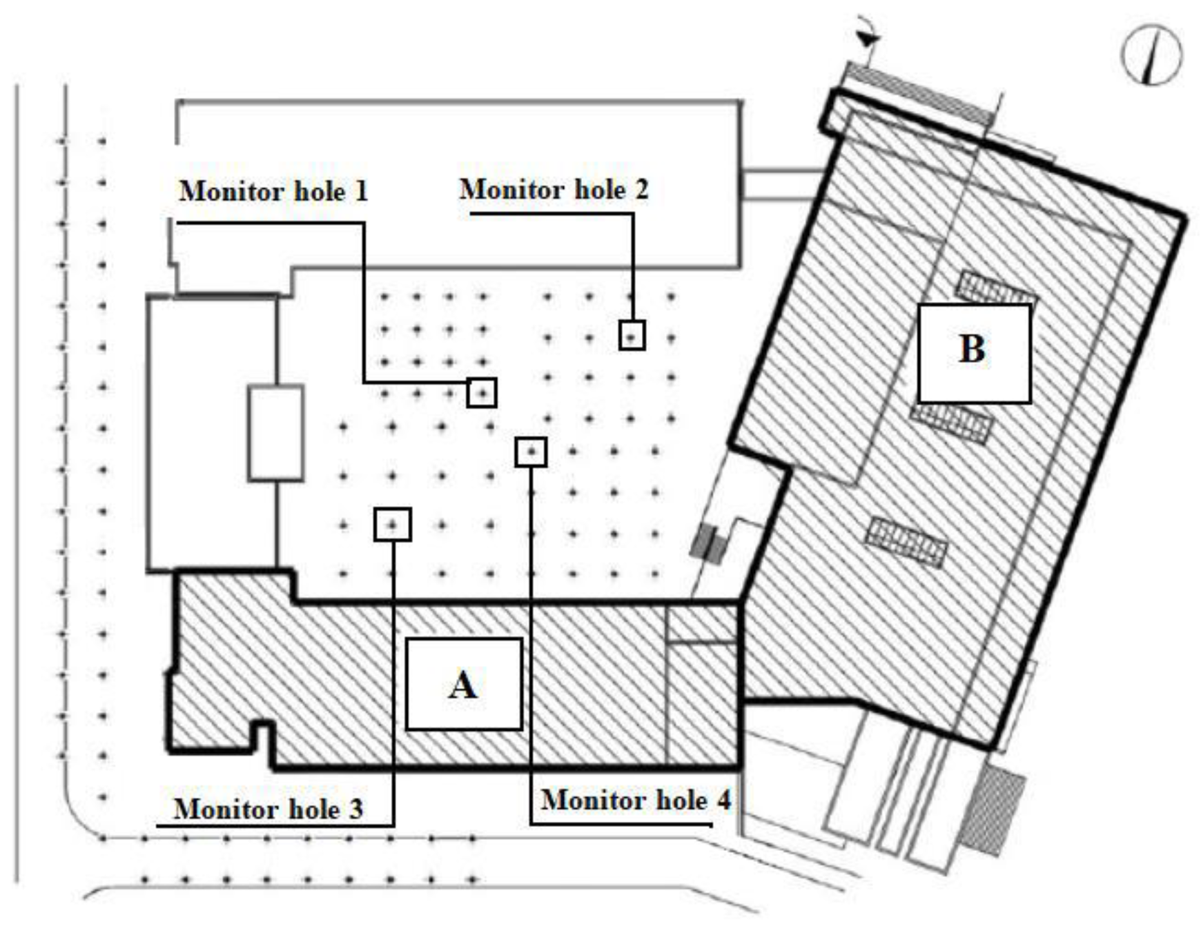
3.1.3. Monitoring of Underground Soil Temperature Data

The monitoring platform is equipped with an outdoor data acquisition base station to monitor the soil temperature at different depths of the heat exchange hole. Monitor hole 1 is set for the heat exchange hole group with a distance of 4 m, Monitor hole 2 and Monitor hole 4 are set for the heat exchange hole groups with distances of 5 m, and Monitor hole 3 is set for the heat exchange hole group with a distance of 6 m, as shown in Figure 2. Three-wire temperature sensors are arranged in the heat exchange hole to realize the ground temperature monitoring at different depths. Eleven temperature sensor measurement points are set underground from 2.5 m to 100 m. The temperature sensor layout in the monitoring well is shown in Figure 5.

3.2. Soil Temperature Simulation Study

In order to further explore the changes in the soil temperature field in well groups with different pipe spacings after the long-term operation of GSHPs, a simulation study is conducted to assess the changes in the soil temperature field after 30 years of operation of the soil source heat pump system. According to the climate and load characteristics of buildings in Changchun, the annual operation process is divided into four stages. The first stage is the heating condition (from 25 October to 15 April of the next year), the second stage is the heating condition after natural recovery (from 16 April to 31 May), the third stage is the cooling condition (from 1 June to 31 August), and the fourth stage marks the end of the natural recovery period after cooling (from 1 September to 24 October).

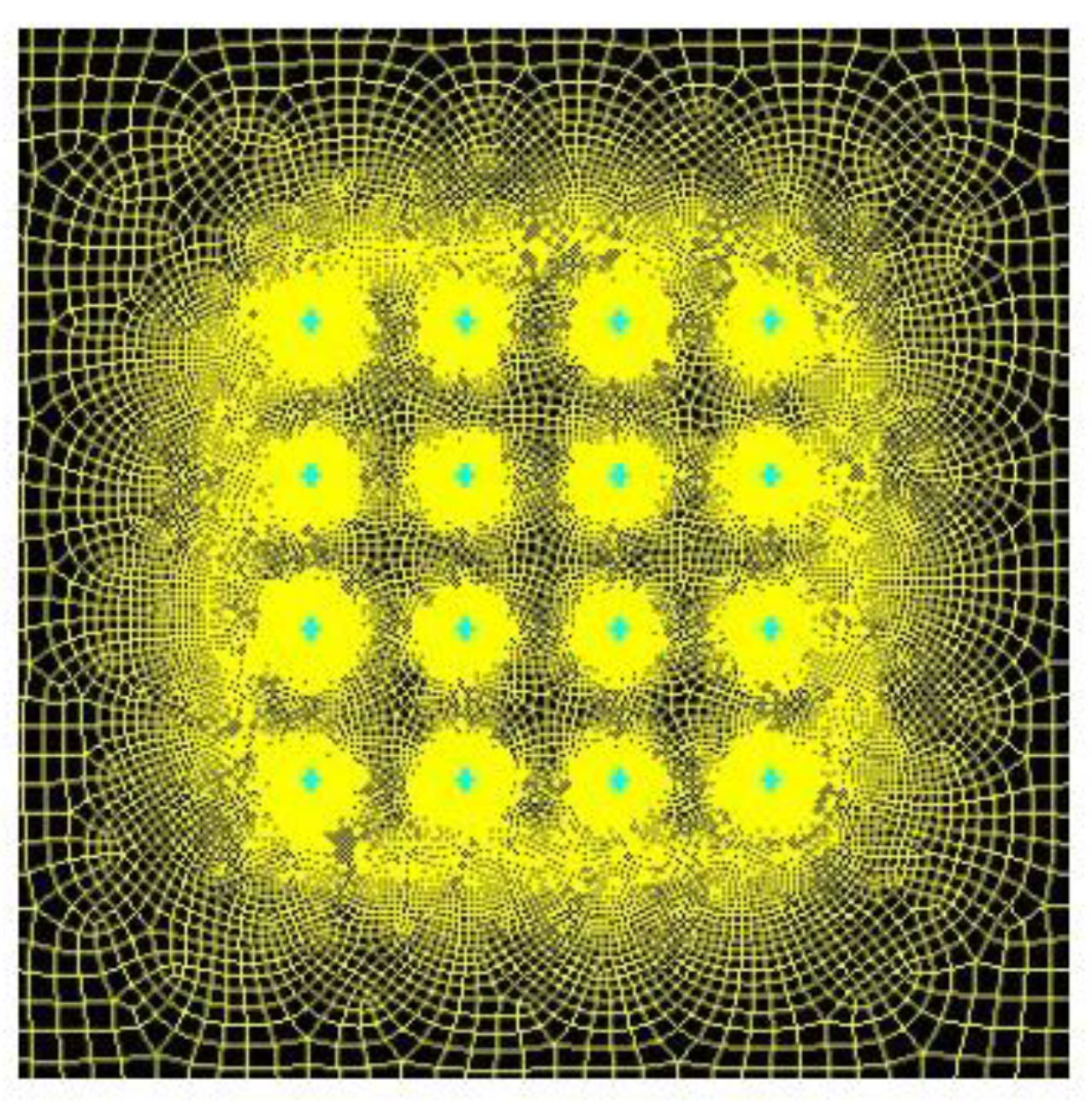
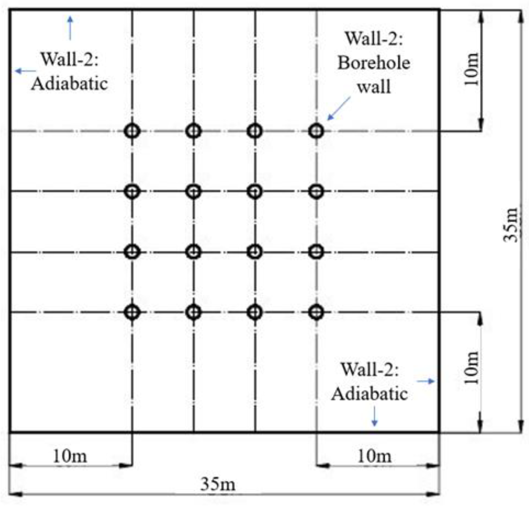
3.2.1. Model Description

The numerical calculation work is carried out using CFD. Using Gambit’s own meshing function, the cells around the buried pipe are divided into a mesh of the appropriate size required for calculation purposes. The mesh files are transferred to Fluent, the post-processing software of Ansys 15.0. Fluent is a software package based on the finite volume method that allows incompressible and compressible fluids to be calculated in a variety of reference systems, flow field simulations, laminar and turbulent flow simulations, constant and non-constant flow analyses, multiphase flow analyses, porous media, heat transfer and thermal mixing analyses, coupled solid and fluid heat transfer analyses, solid and fluid coupled heat transfer analyses, etc. The approach is as follows: Select the FLUENT5/6 solver and define the circulating water as “Fluid” and the HDPE pipe, backfill material, and soil as “Solid”. Define the inlet of the buried pipe as “VELOCITY INLET”, the outlet as “OUTFLOW”, and the other boundaries as “WALL”. Export the model mesh file and read it into the FLUENT solver for calculation. In the FLUENT solver, first check the mesh with the “check” command, and smooth the mesh if necessary. Then define the solver as “Pressure Based”, “Implicit”, and select the “k-epsilon(2eqn)” model. After that, the mathematical model, the material parameters for different zones, the cell zone conditions, the boundary conditions about the fluid zone, etc., are set up.

According to the actual size, the model of the whole heat exchange hole group is established, including a U-shaped pipe, a borehole, a backfill area, and surrounding soil. A rectangular well group with buried pipe spacings of 4 m, 5 m, and 6 m is selected for the simulation study. The well group is arranged in 4 rows and 4 columns, and 16 buried pipe heat exchangers are evenly distributed. The drilling depth is 100 m, the aperture is 0.18 m, the buried pipe is 32 mm, and the heat exchanger spacing and the distance between the heat exchanger and the soil boundary are 5 m. Since the soil temperature change around the buried pipe heat exchanger is the main purpose of this simulation, small unit grids are used for intensive division purposes, and the soil temperature change range around the well group is small, so large grids can be used for division purposes. Fluent software is used for the numerical simulation of the soil temperature field model [24]. The distribution of the soil temperature field around the buried tube heat exchanger is obtained. Figure 6 shows the regional grid division for solving the heat exchange hole group with 5 m spacing.

3.2.2. Governing Equation

The circulating medium in the U-tube is circulated in the heat pump unit using the power of the water pump, so the heat transfer between the circulating medium and the tube wall is the forced convection heat transfer. A large convective heat transfer coefficient, which is necessary for effective heat transfer, can only be achieved when the medium in the tube is in a turbulent state. The parameters for building the k-epsilon(2eqn) turbulence model are shown in

Table 4. k-epsilon(2eqn) turbulence model parameters.

Cum	C1-Epsilon	C2-Epsilon	TKE Prandtl Number	TDR Prandtl Number
0.09	1.44	1.92	1	1.3

. Then, the solver is defined as “Pressure Based”, “Implicit”, and the “k-epsilon(2eqn)” model is selected. Turbulent flow is a state of fluid motion in which the fluid exhibits irregular and chaotic vortex motion. The turbulent state is essential for achieving large convective heat transfer coefficients. It effectively promotes heat transfer and heat transfer efficiency by increasing fluid mixing, expanding the heat transfer surface area, breaking boundary layer restrictions, and reducing heat transfer resistance. The medium in the U-shaped tube can be assumed to be incompressible fluid. The forced flow heat transfer of the circulating medium during the operation of GSHPs can be described by the continuity Equation (14), the momentum Equations (15)–(17), and the energy Equation (18).

The main basis of the continuity equation is that the amount of fluid entering the control body should be balanced with the amount of variation throughout the region. The equation is as follows:

$$\frac{\partial u}{\partial x}+\frac{\partial v}{\partial y}+\frac{\partial w}{\partial z}=0$$

(14)

The momentum equation is mainly based on Newton’s second law and the law of the conservation of momentum. This equation can express the combined forces on the fluid in motion using the rate of change in momentum. In the study of fluid microclusters, the force inside the fluid is much larger than the gravitational force exerted from outside, so the gravity factor is not considered to simplify the calculation, which is expressed as follows:

$$\frac{\partial u}{\partial t}+u\frac{\partial u}{\partial x}+v\frac{\partial u}{\partial y}+w\frac{\partial u}{\partial z}=\upsilon (\frac{{\partial }^{2}u}{\partial x^2}+\frac{{\partial }^{2}u}{\partial y^2}+\frac{{\partial }^{2}u}{\partial z^2})-\frac{1}{\rho }\frac{\partial p}{\partial x}$$

(15)

$$\frac{\partial v}{\partial t}+u\frac{\partial v}{\partial x}+v\frac{\partial v}{\partial y}+w\frac{\partial v}{\partial z}=\upsilon (\frac{{\partial }^{2}v}{\partial x^2}+\frac{{\partial }^{2}v}{\partial y^2}+\frac{{\partial }^{2}v}{\partial z^2})-\frac{1}{\rho }\frac{\partial p}{\partial y}$$

(16)

$$\frac{\partial w}{\partial t}+u\frac{\partial w}{\partial x}+v\frac{\partial w}{\partial y}+w\frac{\partial w}{\partial z}=\upsilon (\frac{{\partial }^{2}w}{\partial x^2}+\frac{{\partial }^{2}w}{\partial y^2}+\frac{{\partial }^{2}w}{\partial z^2})-\frac{1}{\rho }\frac{\partial p}{\partial z}$$

(17)

The energy equation is established on the basis of energy conversion and the law of conservation of energy. The equation mainly reflects the idea that the energy of the inflow and outflow of micro-elements is conserved, which is expressed as:

$$\frac{\partial T}{\partial t}+u\frac{\partial T}{\partial x}+v\frac{\partial T}{\partial y}+w\frac{\partial T}{\partial z}=\alpha (\frac{{\partial }^{2}w}{\partial x^2}+\frac{{\partial }^{2}w}{\partial y^2}+\frac{{\partial }^{2}w}{\partial z^2})$$

(18)

where x, y, and z are the right-angle coordinates in three coordinate directions, m; u, v, and w are the flow velocities in three right-angle coordinate directions, s; $\rho$ is the density, kg/m³; t is the time, s; $v$ is the dynamic viscosity, Pa-s; P is the pressure on the fluid micro-element, Pa; T is the temperature, and k; the is thermal diffusivity, m²/s.

3.2.3. Model Simplification

After the soil thermal property measurement, the results show that the soil distribution around the heat exchanger is as follows: 0–8 m: the loose stratum is mainly clay and powder clay, belonging to the Fourth Series; 8–23 m: coarse sand and medium coarse sand, belonging to the Fourth Series; 23–49 m: moderately weathered and weakly weathered mudstone and sand conglomerate, belonging to the Cretaceous; and 49–92 m: slightly weathered mudstone and sand conglomerate, which is hard and difficult to drill, belonging to the Cretaceous. Since the heat transfer of the vertical U-shaped buried tube heat exchanger and the surrounding soil is related to the type, water content, thermal parameters, cumulative heat, and cold load of the building and other factors, we define the borehole wall as wall-1 and the outer boundary of the soil as wall-2. The heat transfer at the outer boundary of the soil has a weak effect on the heat exchanger and causes negligible temperature fluctuations, so the outer edge of the soil is defined as the adiabatic wall, as shown in Figure 7. In order to facilitate the solution, the following simplification is made to establish the model [25]:

(1)

In the whole heat transfer, the average soil physical property parameters are calculated;

(2)

The initial soil temperature is assumed to be uniform;

(3)

The soil density, thermal conductivity, specific heat, and other parameters do not change with soil temperature and depth;

(4)

The thermal migration caused by water migration in the soil is ignored, i.e., the heat transfer mode between the soil and buried pipe is assumed to be pure heat conduction.

4. Results and Discussion

4.1. Performance Analysis

According to the data recorded by the monitoring system, the change in the unit energy efficiency coefficient COP from winter 2013 to summer 2020 was calculated using Formulas (1)–(3), as shown in

Table 5. Unit energy efficiency factor COP.

Running Time (Winter)	Heating Capacity (kW·h)	COP Variation Range	Average COP	Rate of Compliance (%)	Running Time (Summer)	Cooling Capacity (kW·h)	COP Variation Range	Average COP	Rate of Compliance (%)	Electricity Consumption (kW·h)
2013	526,505.98	3.06–5.15	4.37	93.56	2013	-	-	-	-	101,705
2014	531,574.05	3.51–5.38	4.52	95.27	2014	525,873.65	4.22–5.89	4.91	96.75	154,897
2015	437,091.95	3.78–5.22	4.43	93.68	2015	427,107.59	3.74–5.84	4.86	96.52	138,580
2016	527,108.87	3.42–5.15	4.51	92.71	2016	525,365.71	3.76–5.92	4.81	96.34	149,876
2017	530,755.05	3.39–5.16	4.49	91.26	2017	528,973.06	3.95–5.88	4.79	95.48	153,478
2018	527,786.72	3.48–5.01	4.38	91.18	2018	519,234.18	4.05–5.93	4.83	96.02	150,254
2019	531,244.58	3.56–4.95	4.33	89.97	2019	529,723.19	4.08–5.98	4.84	95.23	149,537
2020	426,588.72	3.65–4.84	4.34	89.33	2020	424,518.62	3.72–5.87	4.88	94.98	137,584

, and the change in the system energy efficiency coefficient SPF is shown in

Table 6. System energy efficiency coefficient SPF.

Running Time (Winter)	SPF Variation Range	Average SPF	Rate of Compliance (%)	Running Time (Summer)	SPF Variation Range	Average SPF	Rate of Compliance (%)
2013	2.07–3.76	3.08	97.32	2013	-	-	-
2014	2.09–3.59	3.02	97.46	2014	2.86–3.68	2.95	98.36
2015	2.58–4.07	3.11	98.57	2015	2.51–3.49	2.82	97.78
2016	2.47–3.56	2.95	96.73	2016	2.66–3.74	2.95	97.86
2017	2.12–3.67	2.97	96.62	2017	2.95–3.89	3.18	98.55
2018	2.38–3.71	2.86	95.89	2018	2.78–3.88	2.98	97.72
2019	2.45–3.68	2.92	96.97	2019	2.61–3.79	2.93	96.89
2020	2.23–3.66	2.89	96.88	2020	2.57–3.85	2.95	97.91

. It can be seen from Table 4 that in the long-term operation of the unit, the average COP of the unit in the winter condition decreases year by year. This is because the water supply temperature of the ground-source side continuously decreases during the long-term operation of the unit. In order to reach the designed water supply temperature, more energy is needed, resulting in the COP of the unit. The average COP of the unit in the summer working condition is higher than that in the winter working condition. This is because the low temperature environment of the underground soil is more conducive to the operation of the GSHP in summer. According to the Chinese national standard GB50189-2005, the coefficient of performance (COP) of heat pump units should not be lower than 4.2. According to the Evaluation Standard for Renewable Energy Building Application Projects, the standard energy efficiency ratio for buried pipe ground-source heat pump systems is 2.20 for winter systems and 2.70 for summer systems. After 8 years of long-term operation, compared with the rated COP of 4.2, the COP compliance rate of the system was 89.33% in the winter condition and 94.98% in the summer condition. As shown in Table 5, after 8 years of the system’s long-term operation, the compliance rate of SPF was 96.88% in the winter working condition compared with the rated SPF value of 2.2, and it was 97.91% in the summer working condition compared with the rated SPF value of 2.7, indicating the stable long-term operation of the unit and system with good energy saving. It shows that the system adopts thermal compensation technology, which can allow the system to run efficiently for a long time and prolong the service life of the system.

4.2. Analysis of Energy Saving Benefits

According to the power consumption record of the monitoring system, the energy saving (coal reduction) and pollutant emission reductions in the system are calculated by Formulas (4)–(14), as shown in

Table 7. Energy saving and pollutant reduction.

Running Time (Year)	Winter Energy Saving (Tons of Standard Coal)	Summer Energy Saving (Tons of Standard Coal)	Annual Energy Saving (Tons of Standard Coal)	Annual CO2 Reduction (t)	Annual SO2 Reduction (t)	Annual Soot Reduction (t)
2013	50.96	0	50.96	125.87	1.0192	0.5096
2014	50.22	35.13	85.35	210.81	1.707	0.8535
2015	45.45	36.54	81.99	202.51	1.6398	0.8199
2016	48.54	35.85	84.39	208.44	1.6878	0.8439
2017	50.65	36.72	87.37	215.81	1.7474	0.8737
2018	47.88	34.98	82.86	204.66	1.6572	0.8286
2019	48.36	35.47	83.83	207.06	1.6766	0.8383
2020	46.72	36.11	82.83	204.59	1.6566	0.8283

. It can be seen from the table that the system has been in long-term operation for 8 years. Given the conventional boiler room heating energy saving 388.78 tons of standard coal, compared with the conventional air conditioning refrigeration energy saving 250.8 tons of standard coal, the system has been running for 8 years with a total standard coal energy saving effect of 639.58 tons. According to the average price of thermal coal in previous years, as shown in Figure 8, the cost of thermal coal saved in the winter working condition was CNY 215,367 and that in the summer working condition was CNY 130,538, totaling CNY 345,905, as shown in

Table 8. Coal cost savings.

Running Time (Winter)	Average Thermal Coal Price (CNY/t)	Total Amount (CNY)	Running Time (Summer)	Average Thermal Coal Price (CNY/t)	Total Amount (CNY)
2013	554	28,232	2013	—	—
2014	489	24,558	2014	482	16,933
2015	375	17,044	2015	401	14,653
2016	638	30,969	2016	462	16,563
2017	611	30,947	2017	589	21,628
2018	578	27,675	2018	578	20,218
2019	552	26,695	2019	577	20,466
2020	626	29,247	2020	556	20,077

100 CNY = 14.03 USD = 13.05 EUR (2023.06).

. According to energy saving calculations, as shown in Table 7, after 8 years of operation, the cumulative CO₂ emission reduction in the system was 1579.75 t, the SO₂ emission reduction was 12.79 t, and soot emission reduction was 6.39 t. This shows that the GSHP can reduce a large amount of coal energy, CO₂, and other harmful substance emissions in the long-term operation [26]. The popularization of GSHPs in cold areas can accelerate the adjustment of China’s coal-based energy structure, and has a high popularization and use value.

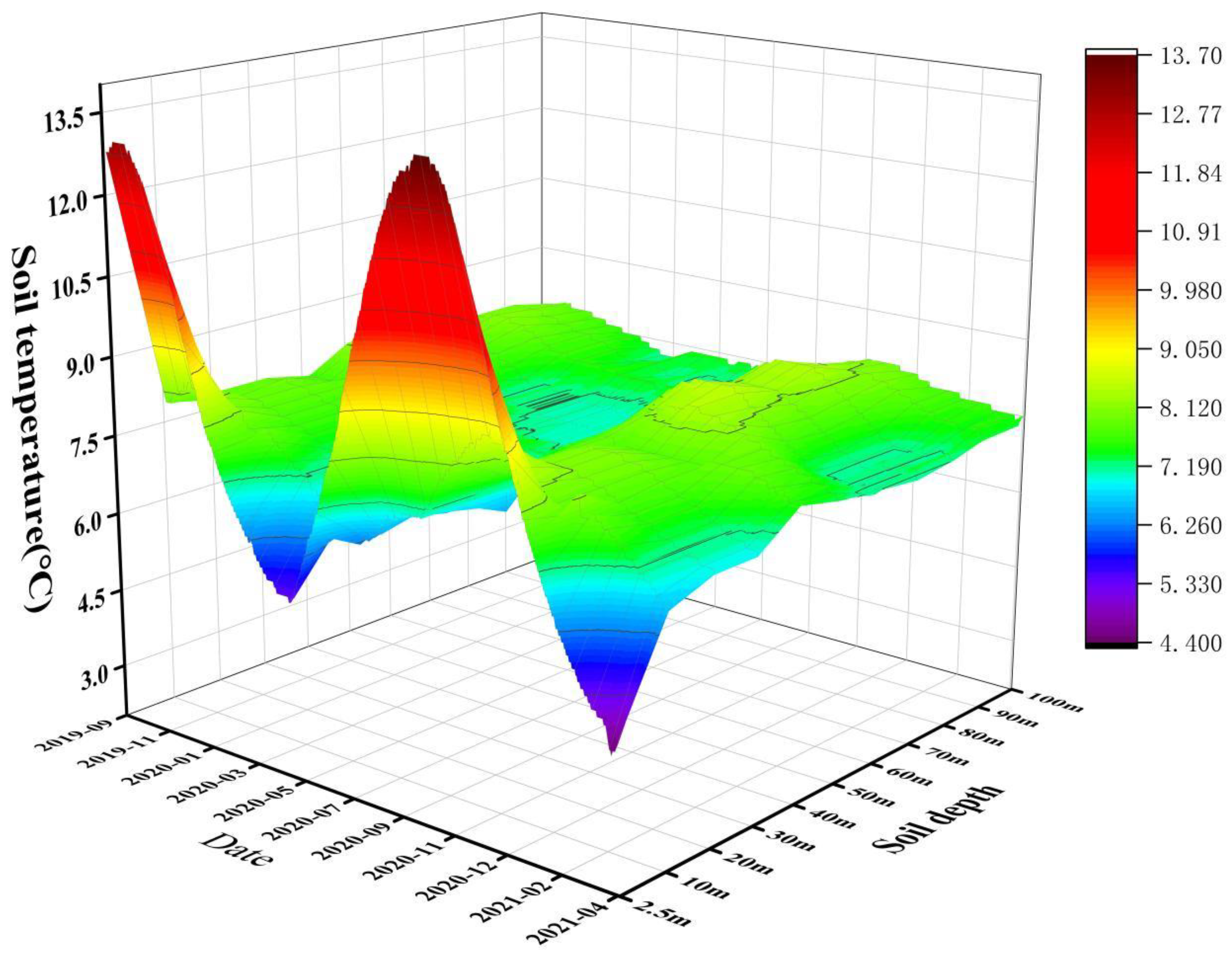
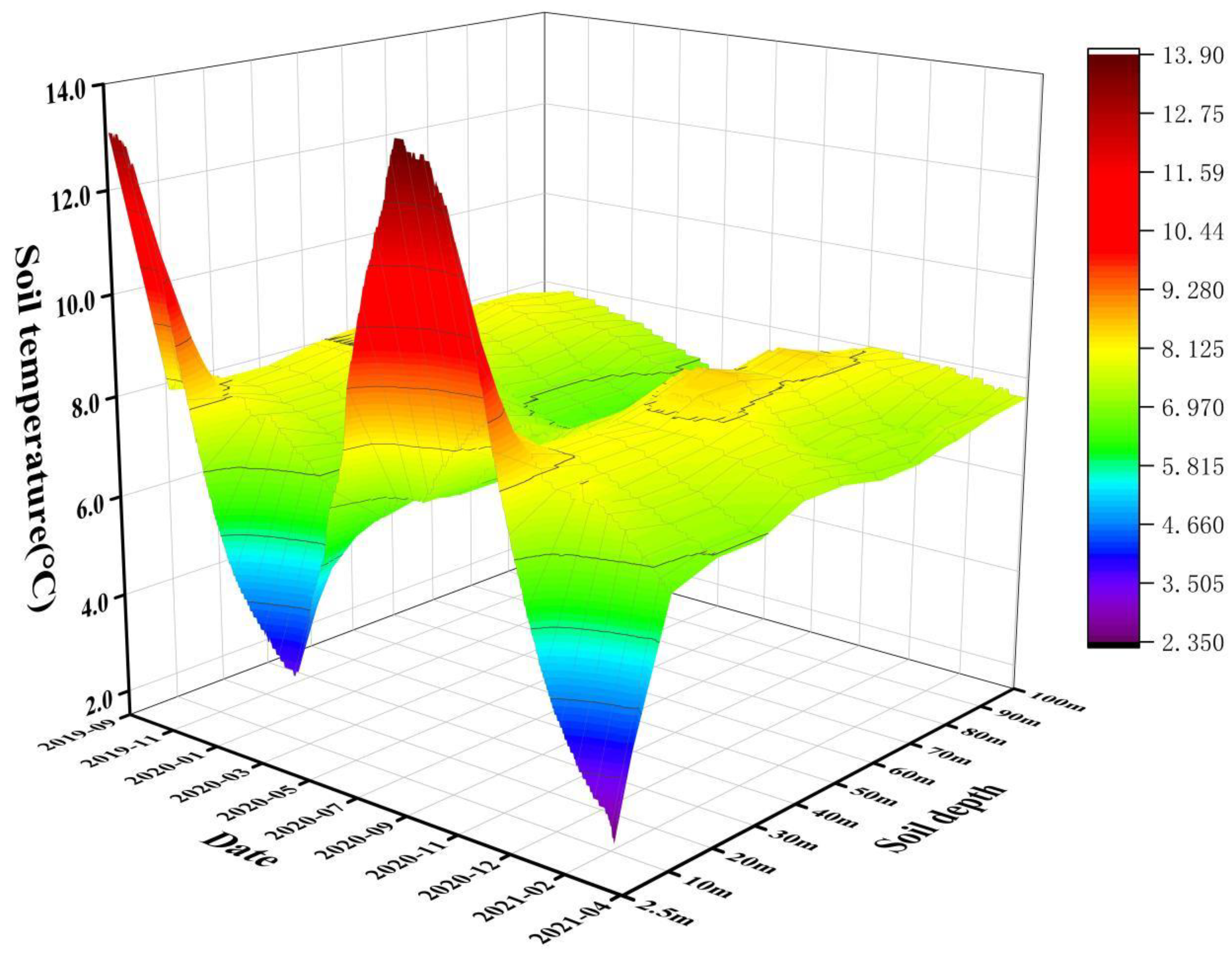
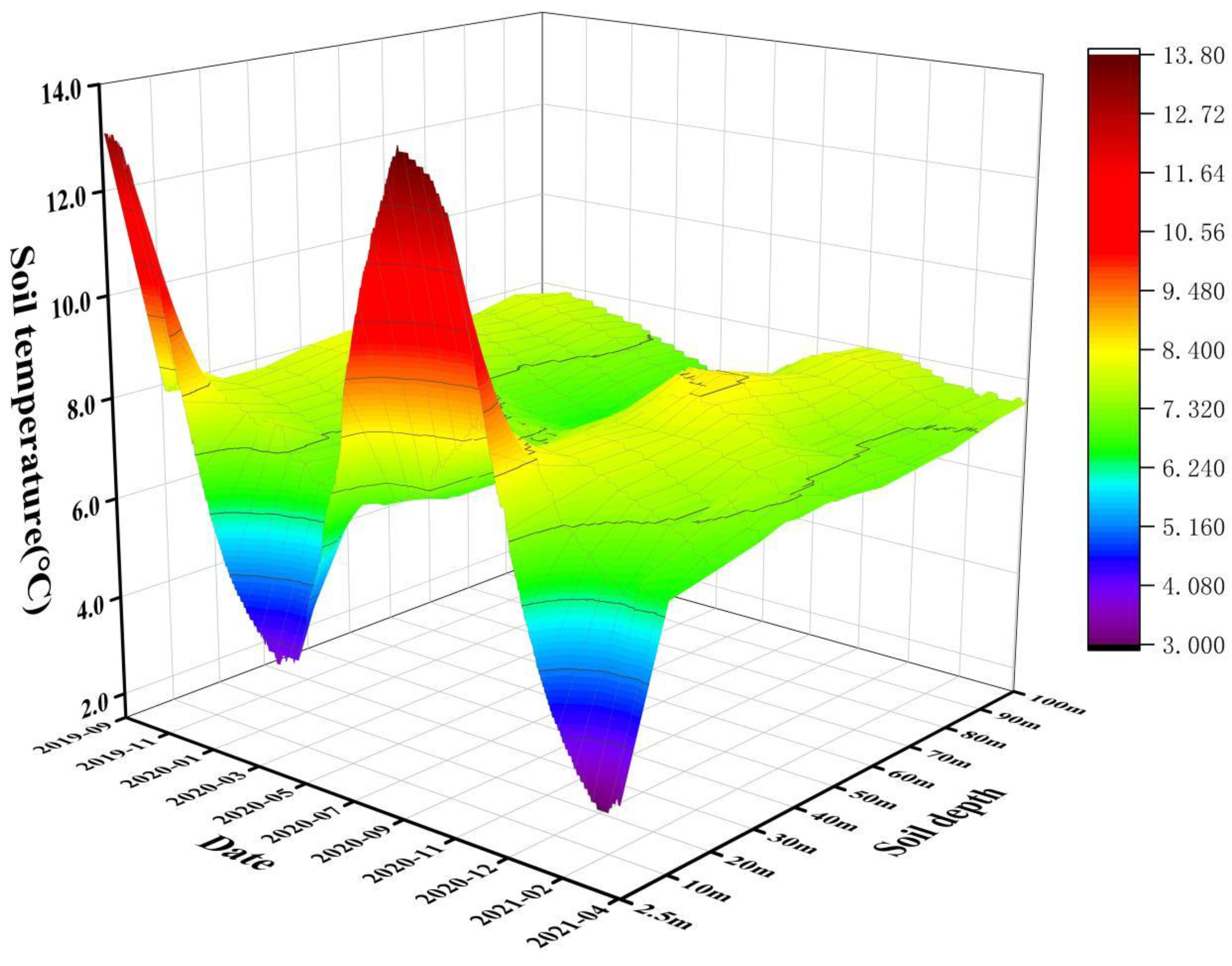
4.3. Analysis of Soil Temperature Monitoring Data

In order to study the soil temperature change, the system’s soil temperature change from the seventh to eighth year of operation was selected from October 2019 to April 2021. According to the data recorded by the soil temperature monitoring system, the heat exchange hole group (Monitor hole 1) with 4 m spacing, the heat exchange hole group (Monitor hole 2) with 5 m spacing, and the heat exchange hole group (Monitor hole 3) with 6 m spacing were selected for a comparative analysis of soil temperature changes in three monitoring holes at different depths. The variations in soil temperature are shown in Figure 9, Figure 10 and Figure 11.

As can be seen from the figure, the soil temperature at the heat exchange holes with distances of 4 m, 5 m, and 6 m presents a basically consistent periodic fluctuation, among which a 2.5 m underground depth has the largest variation range. This situation is caused by the fact that in the shallow underground layer, soil temperature is greatly affected by solar radiation. Meanwhile, the variation range of soil temperature decreases and gradually becomes stable at depths from 10 m to 100 m. Studies have shown that solar radiation is mainly absorbed by the surface soil, which is usually more sensitive to solar radiation and increases in temperature faster. This is because the short-wave radiation from the sun is absorbed at the soil surface and converted into heat energy. With a gradual increase in depth toward the soil, the effect of solar radiation diminishes. Heat is transferred downward in the soil by conduction, making the temperature of deeper soils rise more slowly [27]. Furthermore, soil temperature peaks at a depth of 2.5 m were recorded in October, a trough was recorded in May, soil temperature peaks with depths of 10–100 m were recorded in November, and a trough was recorded in July; thus, shallow soil temperature change lagged for two months or so, and deep soil temperature lagged for about 4 months or so, suggesting that the soil thermal diffusion ability is weak, and that the heat transfer takes a long time. This indicates that the soil temperature cannot be completely recovered during the transition period of 2 to 3 months. After the long-term operation of GSHPs over 8 years, the maximum temperature difference in soil temperature ranged between 0.13 °C and 0.51 °C, and the soil temperature was effectively recovered, which indicates that the area heat compensation technology can effectively solve the problem of soil heat imbalance and extend the service life of the system in cold regions.

According to the monitoring data records, after the system runs until the eighth heating cycle in April 2021, a comparison of the average soil temperatures at various depths around the heat exchange hole and the changes in the initial temperature of soil are shown in Figure 12. The figure shows that the soil temperature of the well group with 4 m heat exchange hole spacing decreased within 0.13 °C~0.51 °C, that of the well group with 5 m pipe spacing decreased within 0.05 °C~0.37 °C, and that of the well group with 6 m heat exchange hole spacing decreased within 0.02 °C~0.38 °C. The figure also shows that the maximum decreasing rates of the soil temperature of the 4 m, 5 m, and 6 m heat exchange hole groups were 2.78%, 2.28%, and 2.02%, respectively, and the variation in the soil temperature in each spacing well group had little difference. Therefore, in the design and construction process of GSHPs in cold regions, 4 m heat exchange hole spacing can be properly considered in the environment of the limited project area, so as to save land use area.

4.4. Simulation Results and Analysis

The temperature field distribution at a 100 m soil depth after the 30th heating cycle of the simulated operation of the well group with 4 m, 5 m, and 6 m spacing is shown in Figure 13. It can be seen from the figure that the drop rate of soil temperature in the heat exchange hole group with 4 m spacing was 26.82%, that in the heat exchange hole group with 5 m spacing was 24.39%, and that in the heat exchange hole group with 6 m spacing was 21.95%. The distribution of the soil temperature field in the three well groups with different spacing is basically similar, and the heat interference in the center of the well group is significant. Compared with the initial soil temperature, the soil temperature around each heat exchange hole also decreased, and the decrease rate of soil temperature between 4 m, 5 m, and 6 m was not different. This was also consistent with the conclusion obtained from practical engineering, further verifying the feasibility of the application of the 4 m heat exchange hole spacing in practical engineering.

Verification of Simulation Results

In order to verify the accuracy of the simulation results, the simulation results at a depth of 40 m were chosen for the analysis, and well sets with 4 m heat exchange borehole spacing and 40 m soil depth were selected, to compare measured and simulated data. Simulated data were selected for cooling conditions from June to August 2020, and for heating conditions from November 2020 to January 2021. The measured data were compared to the simulated data as shown in Figure 14. Figure 12 shows that the soil temperature varied more at a depth of 40 m. The figure also shows that the monitoring data and simulation data had a good fitting degree, and the maximum errors were 2.3% and 2.1%. The variation curve of soil temperature under the cooling condition showed an upward trend, while the curve of soil temperature under the heating condition showed a downward trend. Compared with the measured data, the simulated data curve of soil temperature change was more stable and did not fluctuate much. This is because the simulation process is an ideal state and does not consider the accuracy of monitoring equipment, water, and seepage in soil, as well as the outdoor temperature and other complex impacts.

4.5. Optimization Scheme of Heat Exchange Hole Spacing

Figure 13 shows that the soil temperature around the heat exchanger hole group also decreased to varying degrees. The soil temperature change area affected by the well group with 4 m spacing was 729 m², the soil temperature change area affected by the well group with 5 m spacing was 841 m², and the soil temperature change area affected by the well group with 6 m spacing was 1089 m². This is due to the fact that when the ground-source heat pump system was under operation, the ground-source heat exchanger in the borehole exchanged heat with the soil, absorbing heat for heating or releasing heat for cooling. This will have an effect on the surrounding soil temperature. In the heating mode, the ground-source heat pump system will absorb heat from the soil, causing a slight decrease in the soil temperature around the borehole. In the cooling mode, the system will release heat into the soil, resulting in a slight increase in soil temperature around the borehole. The effect of the borehole on the surrounding soil temperature existed within a certain range; however, the disturbance radius of the borehole increased as the borehole spacing increased, and the extent of the alignment and footprint on the horizontal plane expanded, resulting in a wider range of soil temperature variation. It can be seen that while the 4 m spacing well group saved land use area, its effect on the thermal stability area of the surrounding soil field was less than that of the 5 m and 6 m spacing heat exchange hole groups. Therefore, in cold region GSHP projects, reducing the area of the heat exchange hole group significantly influences the thermal stability of the surrounding soil temperature field and the ecosystem’s stability.

This project was equipped with 120 heat exchange holes. In accordance with the arrangement of 12 × 10, a minimum floor area of 1584 m² was required for all 4 m hole spacings. The minimum floor area of all 5 m hole spacings was 2475 m²; the minimum floor area of all 6 m hole spacings was 3564 m²; the use of 4 m hole spacing was favored over 5 m and 6 m hole spacings to save land areas of 891 m² and 1980 m², respectively; and the minimum floor area was reduced by 36% to 55.5%. This also shows that the use of 4 m hole spacing can save the project area and reduce costs.

5. Conclusions

In this study, the measured data of the GSHP of public buildings in the cold region for a long period of operation over 8 years were organized and analyzed; changes in the COP of the unit and the SPF of the system, as well as the changes in the soil temperature field, were calculated; and the impact of the distance between 4 m, 5 m, and 6 m heat exchange holes on soil thermal stability was compared. CFD software was used to simulate the soil temperature field of three kinds of heat exchange hole spacing after 30 years of system operation, and the simulated values were verified by combining the measured data. Meanwhile, the optimization scheme of the heat exchange hole spacing suitable for the construction of the soil source heat pump in cold regions was proposed. The findings are summarized as follows:

(1)

After the long-term operation of GSHPs over 8 years, the soil temperature difference varied between 0.13 °C and 0.51 °C, and the maximum reduction rate was 2.78%. Because the system uses the area compensation technology, by changing the heating and cooling area, the cold and hot load balance was maintained, and the soil temperature field changes tended to be stable after the long-term operation of the system. The results show that the area compensation technology can effectively alleviate the soil heat imbalance in the cold region.

(2)

In the long-term operation of GSHPs over 8 years, the average COP of the unit in the winter working condition was 4.42, and the compliance rate ranged between 89.33% and 95.27%. The highest COP was 4.52, the lowest COP was 4.33, and the change rate was 4.2%. In summer, the average COP was 4.84, and the compliance rate ranged between 94.98% and 96.75%. The highest COP was 4.91, the lowest COP was 4.79, and the change rate was 2.4%. The results show that the system can maintain the stability of the soil temperature field using area compensation technology, which can effectively guarantee the stable and efficient operation of the system in long-term operation.

(3)

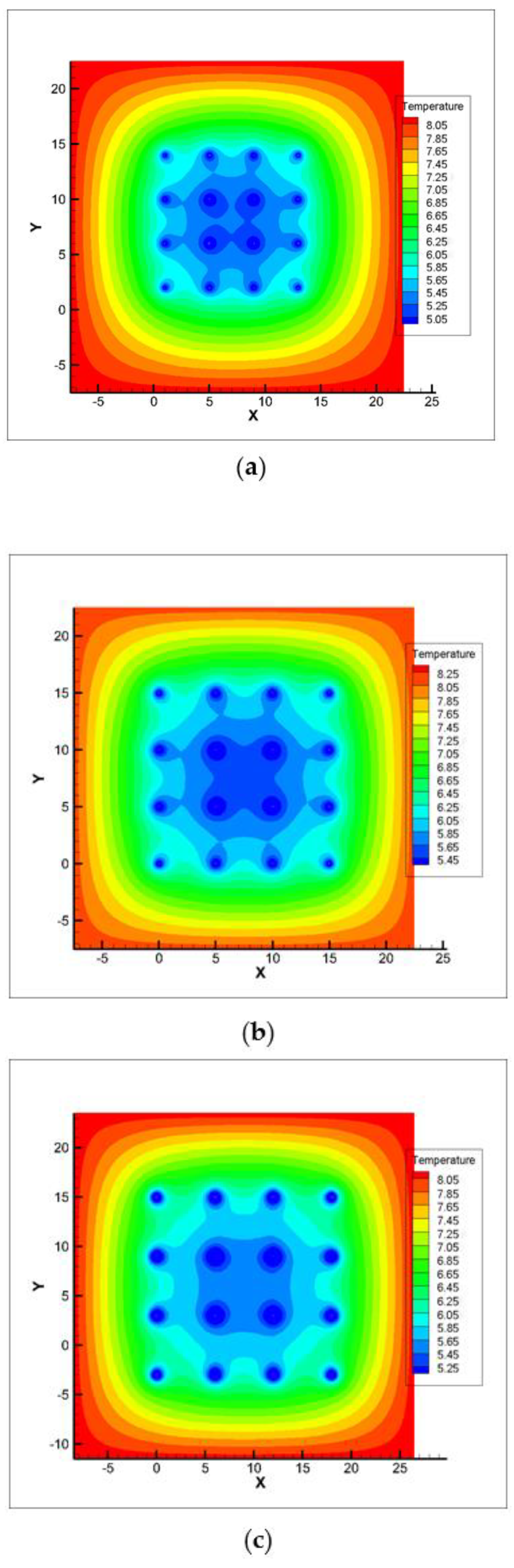
After the area compensation technology was used in the soil source heat pump system, the maximum decrease rates of the soil temperature were 2.78%, 2.28%, and 2.02% after the long-term operation of heat exchange hole groups with different spacings of 4 m, 5 m, and 6 m. After 30 years of the long-term operation of the simulation system, the temperature drop rates of the soil temperature of 100 m with spacings of 4 m, 5 m, and 6 m were 26.82%, 24.39%, and 21.95%. The measured and simulated results show that the three different spaces of the heat transfer hole groups exhibited little differences in the soil temperature change. The results show that in severe cold areas, when the project area of the GSHP is limited, it is not necessary to excessively attempt to increase the heat exchange hole spacing to maintain the heat balance of the soil temperature field. If the heat exchange hole spacing is 4 m, it can still run stably and efficiently when the cold and heat load is balanced using appropriate methods. Taking the actual number of heat exchange holes in the project as an example, the minimum floor area with 4 m heat exchange hole spacing was reduced by 36% and 55.5%, respectively, compared with that of 5 m and 6 m heat exchange hole spacings. This further shows that, by applying soil source heat pump systems in densely populated cities in cold areas and arranging boreholes at 4 m spacings, more boreholes can be accommodated in the same footprint, reducing the total footprint required for the system, which in turn reduces the cost of land occupation and construction costs, as well as horizontal pipe connection costs. Moreover, the smaller footprint reduces disturbance to underground utilities and buildings, which can reduce the additional work and costs associated with underground work. This also facilitates the use and promotion of GSHPs in colder regions.

(4)

After 8 years of the long-term operation of GSHPs, compared with traditional coal-fired boilers and traditional air conditioning methods, the cumulative coal saving amount was 639.58 t, the cumulative CO₂ emission reduction was 1579.75 t, the SO₂ emission reduction was 12.79 t, and the soot emission reduction was 6.39 t. The results show that the use of GSHPs in severe cold regions can effectively reduce the use of coal energy and reduce CO₂ and pollutant emissions, which is of great significance for China to speed up adjustments in its traditional energy structure and promote carbon peak carbon neutralization.

References

1. Wang, W.; Huo, J.-H.; Tao, Y.-T.; Lei, B.; Wu, Y.-T.; Ma, C.-F. Semi-empirical modelling and analysis of single screw expanders considering inlet and exhaust pressure losses. Energy 2023, 266, 126356. [Google Scholar] [CrossRef]
2. Xi, C.; Lin, L.; Hongxing, Y. Long term operation of a solar assisted ground coupled heat pump system for space heating and domestic hot water. Energy Build. 2011, 43, 1835–1844. [Google Scholar] [CrossRef]
3. Yang, W.; Zhou, J.; Xu, W.; Zhang, G. Current status of ground-source heat pumps in China. Energy Policy 2010, 38, 323–332. [Google Scholar] [CrossRef]
4. Hepbasli, A.; Akdemir, O.; Hancioglu, E. Experimental study of a closed loop vertical ground source heat pump system. Energy Convers. Manag. 2003, 44, 527–548. [Google Scholar] [CrossRef]
5. Mousa, M.M.; Bayomy, A.M.; Saghir, M.Z. Long-term performance investigation of a GSHP with actual size energy pile with PCM. Appl. Therm. Eng. 2022, 210, 118381. [Google Scholar] [CrossRef]
6. Deng, Y.; Feng, Z.; Fang, J.; Cao, S.-J. Impact of ventilation rates on indoor thermal comfort and energy efficiency of ground-source heat pump system. Sustain. Cities Soc. 2018, 37, 154–163. [Google Scholar] [CrossRef]
7. Koohi-Fayegh, S.; Rosen, M.A. Examination of thermal interaction of multiple vertical ground heat exchangers. Appl. Energy 2012, 97, 962–969. [Google Scholar] [CrossRef]
8. Yuan, Y.; Cao, X.; Wang, J.; Sun, L. Thermal interaction of multiple ground heat exchangers under different intermittent ratio and separation distance. Appl. Therm. Eng. 2016, 108, 277–286. [Google Scholar] [CrossRef]
9. İnallı, M.; Esen, H. Experimental thermal performance evaluation of a horizontal ground-source heat pump system. Appl. Therm. Eng. 2004, 24, 2219–2232. [Google Scholar] [CrossRef]
10. Blum, P.; Campillo, G.; Münch, W.; Kölbel, T. CO2 savings of ground source heat pump systems–A regional analysis. Renew. Energy 2010, 35, 122–127. [Google Scholar] [CrossRef]
11. Liu, Z.; Xu, W.; Qian, C.; Chen, X.; Jin, G. Investigation on the feasibility and performance of ground source heat pump (GSHP) in three cities in cold climate zone, China. Renew. Energy 2015, 84, 89–96. [Google Scholar] [CrossRef]
12. You, T.; Wu, W.; Shi, W.; Wang, B.; Li, X. An overview of the problems and solutions of soil thermal imbalance of ground-coupled heat pumps in cold regions. Appl. Energy 2016, 177, 515–536. [Google Scholar] [CrossRef]
13. Qian, H.; Wang, Y. Modeling the interactions between the performance of ground source heat pumps and soil temperature variations. Energy Sustain. Dev. 2014, 23, 115–121. [Google Scholar] [CrossRef]
14. Yu, T.; Liu, Z.; Chu, G.; Qu, Y. Influence of Intermittent Operation on Soil Temperature and Energy Storage Duration of Ground-Source Heat Pump System for Residential Building. In Proceedings of the 8th International Symposium on Heating, Ventilation and Air Conditioning; Springer: Berlin/Heidelberg, Germany, 2014; pp. 203–213. [Google Scholar]
15. You, T.; Wang, B.; Wu, W.; Shi, W.; Li, X. Performance analysis of hybrid ground-coupled heat pump system with multi-functions. Energy Convers. Manag. 2015, 92, 47–59. [Google Scholar] [CrossRef]
16. Shang, Y.; Dong, M.; Li, S. Intermittent experimental study of a vertical ground source heat pump system. Appl. Energy 2014, 136, 628–635. [Google Scholar] [CrossRef]
17. Retkowski, W.; Ziefle, G.; Thöming, J. Evaluation of different heat extraction strategies for shallow vertical ground-source heat pump systems. Appl. Energy 2015, 149, 259–271. [Google Scholar] [CrossRef]
18. Kurevija, T.; Vulin, D.; Krapec, V. Effect of borehole array geometry and thermal interferences on geothermal heat pump system. Energy Convers. Manag. 2012, 60, 134–142. [Google Scholar] [CrossRef]
19. Yang, C.; Zhu, W.; Sun, J.; Xu, X.; Wang, R.; Lu, Y.; Zhang, S.; Zhou, W. Assessing the effects of 2D/3D urban morphology on the 3D urban thermal environment by using multi-source remote sensing data and UAV measurements: A case study of the snow-climate city of Changchun, China. J. Clean. Prod. 2021, 321, 128956. [Google Scholar] [CrossRef]
20. Daemi, N.; Krol, M.M. Impact of building thermal load on the developed thermal plumes of a multi-borehole GSHP system in different canadian climates. Renew. Energy 2019, 134, 550–557. [Google Scholar] [CrossRef]
21. Liu, X.; Ren, H.; Wu, Y.; Kong, D. An analysis of the demonstration projects for renewable energy application buildings in China. Energy Policy 2013, 63, 382–397. [Google Scholar] [CrossRef]
22. Sang, J.; Liu, X.; Liang, C.; Feng, G.; Li, Z.; Wu, X.; Song, M. Differences between design expectations and actual operation of ground source heat pumps for green buildings in the cold region of northern China. Energy 2022, 252, 124077. [Google Scholar] [CrossRef]
23. Nouri, G.; Noorollahi, Y.; Yousefi, H. Designing and optimization of solar assisted ground source heat pump system to supply heating, cooling and hot water demands. Geothermics 2019, 82, 212–231. [Google Scholar] [CrossRef]
24. Ma, G.; Gu, F.; Gu, J.; Li, X. Numerical Simulation on Soil Temperature Field around Underground Hot Oil Pipelines and Medium Temperature-Drop in the Process of Staring. In ICPTT 2009; American Society of Civil Engineers: Reston, VA, USA, 2009; pp. 373–380. [Google Scholar]
25. Gao, Z.; Hu, Z.; Chen, T.; Xu, X.; Feng, J.; Zhang, Y.; Su, Q.; Ji, D. Numerical study on heat transfer efficiency for borehole heat exchangers in Linqu County, Shandong Province, China. Energy Rep. 2022, 8, 5570–5579. [Google Scholar] [CrossRef]
26. Michopoulos, A.; Zachariadis, T.; Kyriakis, N. Operation characteristics and experience of a ground source heat pump system with a vertical ground heat exchanger. Energy 2013, 51, 349–357. [Google Scholar] [CrossRef]
27. Yao, X.P. Study and Numerical Analysis of Soil Temperature Field of Soil Source Heat Pump Heat Exchanger in Cold Regio. Master’s Thesis, Harbin University of Commerce, Harbin, China, 2020. [Google Scholar]
Figure 1. Satellite view of the building.
Buildings 13 01564 g001
Figure 2. Annual outdoor temperature change curve.
Buildings 13 01564 g002
Figure 3. Heating and cooling zoning and underground heat transfer well layout.
Buildings 13 01564 g003
Figure 4. Monitoring system data center.
Buildings 13 01564 g004
Figure 5. Monitor well temperature sensor layout.
Buildings 13 01564 g005
Figure 6. Grid computing area.
Buildings 13 01564 g006
Figure 7. Boundary conditions.
Buildings 13 01564 g007
Figure 8. Thermal coal prices in China.
Buildings 13 01564 g008
Figure 9. Soil temperature changes in 4 m interval wells from September 2019 to April 2021.
Buildings 13 01564 g009
Figure 10. Soil temperature changes in 5 m interval wells from September 2019 to April 2021.
Buildings 13 01564 g010
Figure 11. Soil temperature changes in 6 m interval wells from September 2019 to April 2021.
Buildings 13 01564 g011
Figure 12. Soil temperature changes after the end of the heating period in April 2021.
Buildings 13 01564 g012
Figure 13. The soil temperature field after 30 years of operation was simulated with heat exchanger holes with distances of 4 m, 5 m, and 6 m. ((a). 4 m Heat exchange hole spacing; (b). 5 m Heat exchange hole spacing; (c). 6 m Heat exchange hole spacing).
Buildings 13 01564 g013
Figure 14. Comparison of actual values and simulated values under cooling conditions and heating conditions. ((a). Comparison of actual and simulated values of cooling conditions; (b). Comparison of actual and simulated values of heating conditions).
Buildings 13 01564 g014