Analyzing the Effect of Rotary Inertia and Elastic Constraints on a Beam Supported by a Wrinkle Elastic Foundation: A Numerical Investigation

Abstract

This article presents a modal analysis of an elastically constrained Rayleigh beam that is placed on an elastic Winkler foundation. The study of beams plays a crucial role in building construction, providing essential support and stability to the structure. The objective of this investigation is to examine how the vibrational frequencies of the Rayleigh beam are affected by the elastic foundation parameter and the rotational inertia. The results obtained from analytical and numerical methods are presented and compared with the configuration of the Euler–Bernoulli beam. The analytic approach employs the technique of separation of variable and root finding, while the numerical approach involves using the Galerkin finite element method to calculate the eigenfrequencies and mode functions. The study explains the dispersive behavior of natural frequencies and mode shapes for the initial modes of frequency. The article provides an accurate and efficient numerical scheme for both Rayleigh and Euler–Bernoulli beams, which demonstrate excellent agreement with analytical results. It is important to note that this scheme has the highest accuracy for eigenfrequencies and eigenmodes compared to other existing tools for these types of problems. The study reveals that Rayleigh beam eigenvalues depend on geometry, rotational inertia minimally affects the fundamental frequency mode, and linear spring stiffness has a more significant impact on vibration frequencies and mode shapes than rotary spring stiffness. Further, the finite element scheme used provides the most accurate results for obtaining mode shapes of beam structures. The numerical scheme developed is suitable for calculating optimal solutions for complex beam structures with multi-parameter foundations.

1. Introduction

Structural elements such as beams are widely used in geotechnical, civil, and mechanical engineering because they can simulate the behavior of various structures. These structures are frequently used and modeled on elastic foundations for isolation purposes, to study the dynamics of buildings on the ground or in railway applications. To optimally design these structures, it is always necessary to know their dynamic characteristics. Given this, vibration analysis of beams on elastic foundations is a valuable study that can be used in various structural engineering applications.

To start with, the dynamic response of the beams without elastic foundations has been extensively studied by a number of researchers. Chun [1] presented the free vibration of the beam attached to the rotational spring at one end and by letting the other end free. Lee [2] derived the characteristic equation of a beam having a rotational spring at one end and the other free end with an attached mass. Lai et al. [3] used the Adomian decomposition method to solve the beam vibration problem. A sinc-Galerkin method was presented by Smith et al. [4] to solve the beam problems having fixed boundary conditions where authors demonstrated that sinc discretization was particularly suited for beam problems yielding the best numerical results. Hess [5] extended the investigation to a beam with symmetrical spring-hinged ends. Grossi and Arenas [6] introduced both optimized Rayleigh–Schmidt and Rayleigh–Ritz methods to obtain the frequencies with changing height and width. The approximate solution of a beam under linearly changing axial force was established by Naguleswaran [7,8]. He also expanded this approach to searching the natural frequencies and eigenmodes of the Euler–Bernoulli beam (EBB) varying in cross-sections up to three steps. Laura et al. [9] studied the axial force on beams carrying concentrated masses. Abbas [10] investigated the dynamical analysis of Timoshenko beams having non-classical boundary conditions. Rao and Naidu [11] investigated the stability behavior of uniform columns and beams with nonlinear rotational and elastic constraints. Buckling analyses of beams utilizing differential quadrature and harmonic differential quadrature have been performed by Civalek [12]. Frequency parameters of the beam for non-classical conditions were determined using a Fourier method [13]. In [14], the damped beam study was investigated for a non-classical case employing the Fourier cosine series for the determination of dynamical responses while the fractional approach was implicated on the investigation of a Euler–Bernoulli (EB) beam in [15]. Later came a study about the free double beam with forcing and different conditions associated with the discrete points and a viscoelastic layer [16]. Overall, these studies have investigated various aspects of beam dynamics using different techniques, including free vibration, characteristic equations, Adomian decomposition, sinc-Galerkin method, symmetrical spring-hinged ends, optimized Rayleigh–Schmidt and Rayleigh–Ritz methods, axial force, non-classical boundary conditions, stability behavior, buckling analyses, Fourier method, deflection by fractional differential equation, and double beam vibration with a viscoelastic layer and discrete points.

The interaction of structures with the foundations has been thoroughly discussed by many researchers. Wang [17] investigated the vibration of stepped beams on elastic foundations, while Lai et al. [18] studied the dynamic response of beams on elastic foundations. Extensive research was conducted on the behavior of beams supported by elastic foundations [19]. A model for flexible foundations involving two parameters was reinvestigated [20], while the fundamental solution to examine the response of thick plates over a Winkler-type foundation was extracted utilizing the boundary element approach [21]. An efficient analytical approach to analyze vibrations in beams on an elastic foundation with restrained ends was also intended [22]. The dynamic characteristics and dispersion properties of an elastic five-layered plate subjected to anti-plane shear vibrations, using an asymptotic approach and considering interfacial imperfections were detailed in [23,24]. The homotopy analysis method to accomplish static analysis of composite beams on elastic foundations with variable stiffness was employed in [25]. The analytical solution to study the vibrations of functionally graded beams with varying cross-sections supported by elastic foundations of the Pasternak type was provided in [26]. The free vibration properties in two parallel beams connected through a variable stiffness elastic layer with restrained ends were analyzed in [27]. An inclusive review of recent studies concerning the analysis of free vibrations and stability in functionally graded materials within sandwich plates was conducted in [28]. Additionally, there is a significant part of the literature that examines vibration analysis in numerous structures under different physical conditions, as can be viewed in [29,30].

As revealed from the above review, researchers have used various analytical and computational ways to explore beam vibrations for several situations. These procedures involve eigenfunction expansion, Fourier method, Galerkin, modal analysis, differential transform wavelet, homotopy and adomian decomposition, finite difference and element approaches. While having multiple investigations, research gaps still exist. For example, while some studies focus on elastic foundation effects, little attention has been given to the influence of elastic supports on frequency and amplitude. Moreover, most studies neglect elastically constrained boundary conditions and material nonlinearity. Effectively addressing the complex dynamics associated with beam vibration under diverse conditions poses a formidable challenge in ensuring the reliability and accuracy of solutions. The accuracy of the obtained results is primarily contingent upon the assumptions made during modeling, the prescribed boundary conditions, and the chosen material properties within the study. In order to enhance the precision of predictions, researchers can strive to refine their models by employing more accurate assumptions or by leveraging advanced numerical techniques. Consequently, there remains a need for further research to bridge these gaps and develop more precise and efficient models for the analysis of beam vibrations on elastic foundations under various boundary conditions. The objective of the present study is aligned with this pursuit, aiming to address these research gaps and contribute to the development of improved methodologies for analyzing beam vibrations on elastic foundations.

This study is primarily focused on conducting an extensive modal analysis of a Rayleigh beam subjected to elastic constraints and positioned on an elastic Winkler foundation. The main aim is to investigate how the inclusion of rotational inertia influences the modal behavior and dynamic response of the beam. By carefully considering the combined effects of elastic constraints and the foundation’s elasticity, the study aims to offer significant aid to the modal characteristics and overall behavior of the beam system. The solution to the underlying problem is derived with the best accuracy by using a finite element scheme for initial modes of the vibrating frequency with and without considering the Winkler elastic foundation. The frequency curve, natural frequencies, and corresponding mode shapes are sketched for various situations depicting the deflection behavior of the beam. The primary objective and novelty of this study is to establish a numerical scheme with the best accuracy so that the more complex nature of beam structures can be dealt with in such a scheme appropriately. The research is significant as it provides a prototype for obtaining optimal solutions for structural problems containing rotary and shear deformation effects simultaneously with dynamical boundary conditions. The findings of this study can be useful in determining optimal values of eigenfrequencies and eigenmodes for forced vibration problems of beams resting on multiparametric foundations. The study has applications in various fields such as civil engineering, mechanical engineering, and aerospace engineering. Understanding the vibrational behavior of beams on elastic foundations is crucial in the design of various structures, including buildings, bridges, and aircraft. The findings from this study can be applied to improve the accuracy of modeling and simulation tools used in structural analysis, which can lead to more efficient and cost-effective designs.

The rest of the article is organized as follows. Section 2 contains the governing problem. Section 3 states a working procedure for calculating eigenfrequencies, eigenvalues, and eigenmodes. The results are presented and discussed in Section 4, whereas the conclusion is provided in Section 5.

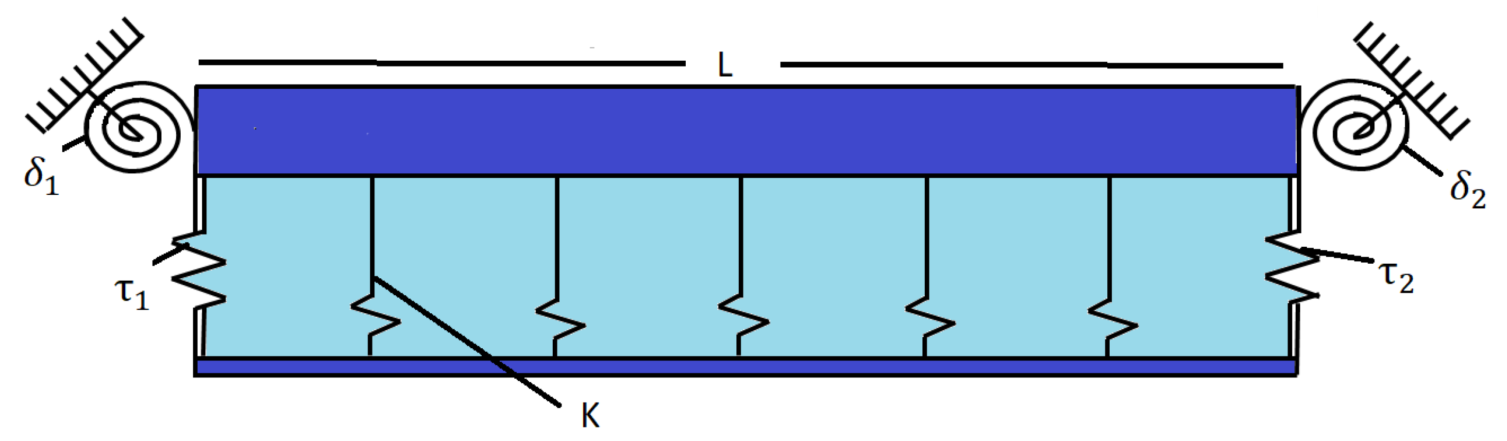
2. Statement of the Problem

Consider a Rayleigh beam (RB) that is attached to linear and rotational springs and resting on a Winkler elastic foundation as shown in Figure 1. Considering the Rayleigh beam theory, the equation of motion for a uniform Rayleigh beam [31] containing the homogeneous material properties is given by

$$EI\frac{{\partial }^4\nu (x,t)}{\partial x^4}+\rho A\frac{{\partial }^2\nu (x,t)}{\partial t^2}-\rho I\frac{{\partial }^4\nu (x,t)}{\partial x^2\partial t^2}+K\nu (x,t)=0,$$

(1)

where $\rho$, I, A, $\nu$, x, t, K, and E are mass density, second moment of inertia, the cross-section area of the beam, displacement of Rayleigh beam, space coordinate, time, stiffness of the Winkler elastic foundation per unit length, and Young’s modulus, respectively. Rotational and linear springs are used to elastically restrained the beam resting on an elastic foundation. Accordingly, the boundary conditions (BC) are given as [31]:

$$\begin{array}{ccc}\hfill EI\frac{{\partial }^3\nu (0,t)}{\partial x^3}-\rho I\frac{{\partial }^3\nu (0,t)}{\partial x\partial t^2}& =& -{\tau }_1\nu (0,t),\hfill \end{array}$$

(2)

$$\begin{array}{ccc}\hfill EI\frac{{\partial }^3\nu (L,t)}{\partial x^3}-\rho I\frac{{\partial }^3\nu (L,t)}{\partial x\partial t^2}& =& {\tau }_2\nu (L,t),\hfill \end{array}$$

(3)

$$\begin{array}{ccc}\hfill EI\frac{{\partial }^2\nu (0,t)}{\partial x^2}& =& {\delta }_1\frac{\partial \nu (0,t)}{\partial x},\hfill \end{array}$$

(4)

$$\begin{array}{ccc}\hfill EI\frac{{\partial }^2\nu (L,t)}{\partial x^2}& =& -{\delta }_2\frac{\partial \nu (L,t)}{\partial x},\hfill \end{array}$$

(5)

where L is the beam’s length, ${\tau }_1$ and ${\tau }_2$ are linear spring constants and ${\delta }_1$ and ${\delta }_2$ are rotational spring constants. It is pertinent to mention here that the equation for the Euler–Bernoulli beam can be obtained by ignoring the rotary inertia effect in Equation (1). Additionally, the boundary conditions stated in Equations (2)–(5) render the classical boundary conditions as a special case by setting the spring constants accordingly. Therefore, the aim of this paper is to determine and analyze the frequency pattern and mode shape of the vibrating beam subject to the boundary condition (2)–(5). Note that the results for classical cases and the EBB are reduced as a special case. The next section explains the analytical and numerical procedure for determining eigenfrequencies and eigenmodes.

3. Determination of Natural Frequencies and Eigenmodes

In this section, we lay out the procedure for the determination of eigenfrequencies and eigenmodes. Numerous researchers used assorted techniques to handle similar problems with certain limitations and compromises on the accuracy of the approximate solutions. Separating the variables is suggested as a way to find frequency relations and eigenfunctions analytically. The root finding technique is then employed to determine eigenvalues and eigenfrequencies for determining respective eigenmodes. The finite element scheme is also used to determine a numerical solution whose validity is to be confirmed through validation.

3.1. Analytic Solution

The method of separation of variables is invoked herein to solve Equation (1). Accordingly, the displacement function is to be separated into two parts as

$$\nu (x,t)=X\left(x\right)T\left(t\right).$$

(6)

Consequently, Equation (1) with the aid of Equation (6) ca be written as

$$EI{X}^{iv}T+\rho AX{T}^{{}^{″}}-\rho I{X}^{{}^{″}}{T}^{{}^{″}}+KXT=0$$

(7)

Furthermore, Equation (7) can be written as [32]

$$\frac{-EI{X}^{\left(4\right)}-KX}{\rho AX-\rho I{X}^{{}^{″}}}=\frac{T^{{}^{″}}}{T}=-{\omega }^2,$$

(8)

where $\omega$ is known as the natural frequency. Equation (8) can be further simplified to render

$$\begin{array}{c}\hfill EI\frac{d^{4}X\left(x\right)}{d{x}^4}+\rho I{\omega }^2\frac{d^{2}X\left(x\right)}{d{x}^2}-({\omega }^2\rho A-K)X=0,\end{array}$$

(9)

and

$$\begin{array}{c}\hfill \frac{d^{2}T\left(t\right)}{d{t}^2}+{\omega }^{2}T\left(t\right)=0.\end{array}$$

(10)

The solution to Equations (9) and (10) is given by

$$\begin{array}{cc}\hfill X\left(x\right)& =Asin\left(\alpha x\right)+Bcos\left(\alpha x\right)+Csinh\left(\beta x\right)+Dcosh\left(\beta x\right),\hfill \end{array}$$

(11)

$$\begin{array}{cc}\hfill T\left(t\right)& =Esin\left(\omega t\right)+Fcos\left(\omega t\right),\hfill \end{array}$$

(12)

where $A,B,C,D,E$, and F are constant coefficients to be determined. The parameters $\alpha$ and $\beta$ above are defined by.

$$\begin{array}{ccc}\hfill \alpha & :=& \sqrt{\frac{\rho I{\omega }^2+\sqrt{{\rho }^2{I}^2{\omega }^4+4EI(\rho A{\omega }^2-K)}}{2EI}},\hfill \end{array}$$

(13)

$$\begin{array}{ccc}\hfill \beta & :=& \sqrt{\frac{\rho I{\omega }^2-\sqrt{{\rho }^2{I}^2{\omega }^4+4EI(\rho A{\omega }^2-K)}}{2EI}}.\hfill \end{array}$$

(14)

Equations (11) and (12), with the help of Equation (6) and the boundary conditions (2)–(5), lead to the system of equations,

$$\begin{array}{cc}\hfill 0=& -AEI\alpha {\beta }^2+B{\tau }_1+CEI{\alpha }^2\beta +D{\tau }_1,\hfill \\ \hfill 0=& A[-\alpha {\beta }^{2}EIcos\left(\alpha L\right)-{\tau }_{2}sin\left(\alpha L\right)]+B[\alpha {\beta }^{2}EIsin\left(\alpha L\right)-{\tau }_{2}cos\left(\alpha L\right)]\hfill \end{array}$$

(15)

$$\begin{array}{cc}\hfill & +C[\alpha {\beta }^{2}EIcosh\left(\beta L\right)-{\tau }_{2}sinh\left(\beta L\right)]+D[{\alpha }^2\beta EIsinh\left(\beta L\right)-{\tau }_{2}cosh\left(\beta L\right)],\hfill \end{array}$$

(16)

$$\begin{array}{cc}\hfill 0=& -A\alpha {\delta }_1-BEI{\alpha }^2-C\beta {\delta }_1+DEI{\beta }^2,\hfill \\ \hfill 0=& A[-{\alpha }^{2}EIsin\left(\alpha L\right)+\alpha {\delta }_{2}cos\left(\alpha L\right)]+B[-{\alpha }^{2}EIcos\left(\alpha L\right)-{\delta }_2\alpha sin\left(\alpha L\right)]\hfill \end{array}$$

(17)

$$\begin{array}{cc}\hfill & +C[{\beta }^{2}EIsinh\left(\beta L\right)+\beta {\delta }_{2}cosh\left(\beta L\right)]+D[{\beta }^{2}EIcosh\left(\beta L\right)+\beta {\delta }_{2}sinh\left(\beta L\right)].\hfill \end{array}$$

(18)

A system of four equations with four unknowns ($A,B,C$, and D) is represented by the Equations (15)–(18). The determinant of the coefficient matrix should be zero in order to find the non-trivial solution. It results in the characteristic equation,

$$\begin{array}{cc}\hfill 0=f(\alpha ,\beta ):=& \left(\right(({\beta }^2{\alpha }^8-{\alpha }^2{\beta }^8)I^4{E}^4-I^2({\beta }^2{\alpha }^6{\delta }_2{\tau }_1+(2{\delta }_2{\tau }_1{\beta }^4+({\tau }_2{\delta }_2+{\tau }_1{\delta }_1)\hfill \\ & {\beta }^2-{\tau }_2{\delta }_1){\alpha }^4+({\delta }_2{\tau }_1{\beta }^6+(-{\tau }_2{\delta }_2-{\tau }_1{\delta }_1{\beta }^4-2{\tau }_2{\delta }_1{\beta }^2){\alpha }^2-{\tau }_2\hfill \\ & {\delta }_1{\beta }^4)E^2-{\tau }_2{\delta }_2{\tau }_1{\delta }_1(\alpha -\beta )(\alpha +\beta ))sin\alpha +EI({\alpha }^2+{\beta }^2)({\beta }^2{I}^2\hfill \\ & ((-{\delta }_2-{\tau }_1){\alpha }^4+{\beta }^2({\tau }_2+{\delta }_1))E^2+{\delta }_2{\tau }_1({\tau }_2+{\delta }_1){\beta }^2-{\tau }_2{\delta }_1({\delta }_2+{\tau }_1))\hfill \\ & \alpha cos\alpha )sinh\beta +\beta (E(-I^2(({\tau }_2+{\delta }_1){\alpha }^2+{\beta }^4\left({\delta }_2+{\tau }_1\right)){\alpha }^2{I}^2\hfill \\ & +{\delta }_2{\tau }_1({\tau }_2+{\delta }_1){\alpha }^2+{\tau }_2{\delta }_1({\delta }_2+{\tau }_1))I({\alpha }^2+{\beta }^2)cosh\beta sin\alpha \hfill \\ & -2\left(\right(I^4{\alpha }^4{\beta }^4{E}^4-1/2(({\delta }_2+{\tau }_1)({\tau }_2+{\delta }_1){\alpha }^4+2{\beta }^2({\tau }_2{\tau }_1+{\delta }_2{\delta }_1){\alpha }^2\hfill \\ & +{\beta }^4({\delta }_2+{\tau }_1)({\tau }_2+{\delta }_1))b^2{a}^2+{\tau }_2{\delta }_2{\tau }_1{\delta }_1(E^2{I}^2{\alpha }^2{\beta }^2+{\tau }_1{\delta }_1)(E^2{I}^2\hfill \\ & {\alpha }^2{\beta }^2+{\tau }_2{\delta }_2\left)\right)\alpha ).\hfill \end{array}$$

(19)

It is essential to note that the characteristic equation is used to calculate the eigenvalues $\alpha$ and $\beta$. Only when $\alpha$ is stated as a function of $\beta$ or otherwise can the explicit values of $\alpha$ or $\beta$ be found. The process outlined below is used to specifically determine the eigenvalues. Equations (13) and (14) define the dispersive relations, which can be expressed as

$$\begin{array}{c}\hfill {\alpha }^2=E_1+\sqrt{E_1^2+E_2},{\beta }^2=-E_1+\sqrt{E_1^2+E_2},\end{array}$$

(20)

where

$$\begin{array}{c}\hfill E_1=\frac{{\omega }^2\rho }{2E},E_2=\frac{{\omega }^2\rho A-K}{EI}.\end{array}$$

(21)

By using Equation (20), we have the expressions

$$\begin{array}{c}\hfill E_1=\frac{{\alpha }^2-{\beta }^2}{2},E_2={\alpha }^2{\beta }^2,\end{array}$$

(22)

which together with (21) furnish

$$\begin{array}{c}\hfill \frac{{\omega }^2\rho }{E}={\alpha }^2-{\beta }^2,\frac{{\omega }^2\rho }{E}=\frac{{\alpha }^2{\beta }^{2}I}{A}+\frac{K}{AE}.\end{array}$$

(23)

Expressions in Equation (23) are made simpler, and the result is

$$\begin{array}{c}\hfill \beta =\sqrt{\frac{{\alpha }^2{u}^2-\frac{K}{EI}}{u^2+{\alpha }^2}},\end{array}$$

(24)

where the slenderness ratio u is described as

$$\begin{array}{c}\hfill u:=L\sqrt{\frac{A}{I}}.\end{array}$$

(25)

Therefore, the eigenvalues of the RB are expressed in the form of a slenderness ratio, which indicates buckling (either pin-jointed or pivoted connections) failure in the beam structure beyond a certain limit. This implies that the eigenvalues in the case of the RB are dependent on the geometry contrary to the EBB, which only depends on the choice of boundary conditions. Hence, the eigenvalue expression (24) together with the slenderness ratio (25) can be written as

$$\begin{array}{c}\hfill \beta =\sqrt{\frac{{\alpha }^2-\frac{K{h}^2}{EI}}{1+{\alpha }^2{h}^2}},\end{array}$$

(26)

where h is the inverse of the slenderness ratio. Given the above procedure, the characteristic Equation (19), together with Equation (26), yields the eigenvalues $\alpha$ and then $\beta$ using a root finding procedure. This further helps in determining the eigenfrequencies using Equation (23). Thus, Equation (11), thanks to Equations (15)–(19), yields the mode function,

$$\begin{array}{c}\hfill S\left(x\right)=D\left[\frac{A}{D}sin\left(\alpha x\right)+\frac{B}{D}cos\left(\alpha x\right)+\frac{C}{D}sinh\left(\beta x\right)+cosh\left(\beta x\right)\right].\end{array}$$

(27)

The eigenvectors for determining $A/D$, $B/D$, and $C/D$ are found by returning to the matrix equation rendered by Equations (15)–(18), and substituting the eigenvalues $\alpha$ and $\beta$ into either of the three equations. Thus, the mode shapes are sketched and analyzed with the help of Equation (27).

As a special case, it is important to observe that by ignoring the stiffness of the elastic foundation and inverse of the slenderness ratio, i.e., $h=K=0$, the problem is reduced to the EBB consideration where eigenvalues are explicitly determined and are independent of the beam geometry since both $\alpha$ and $\beta$ become identical.

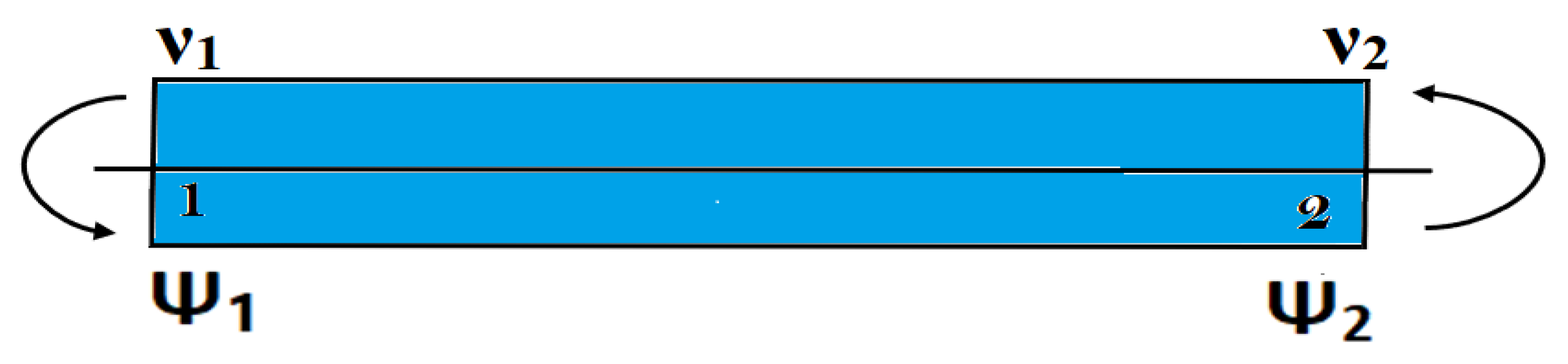
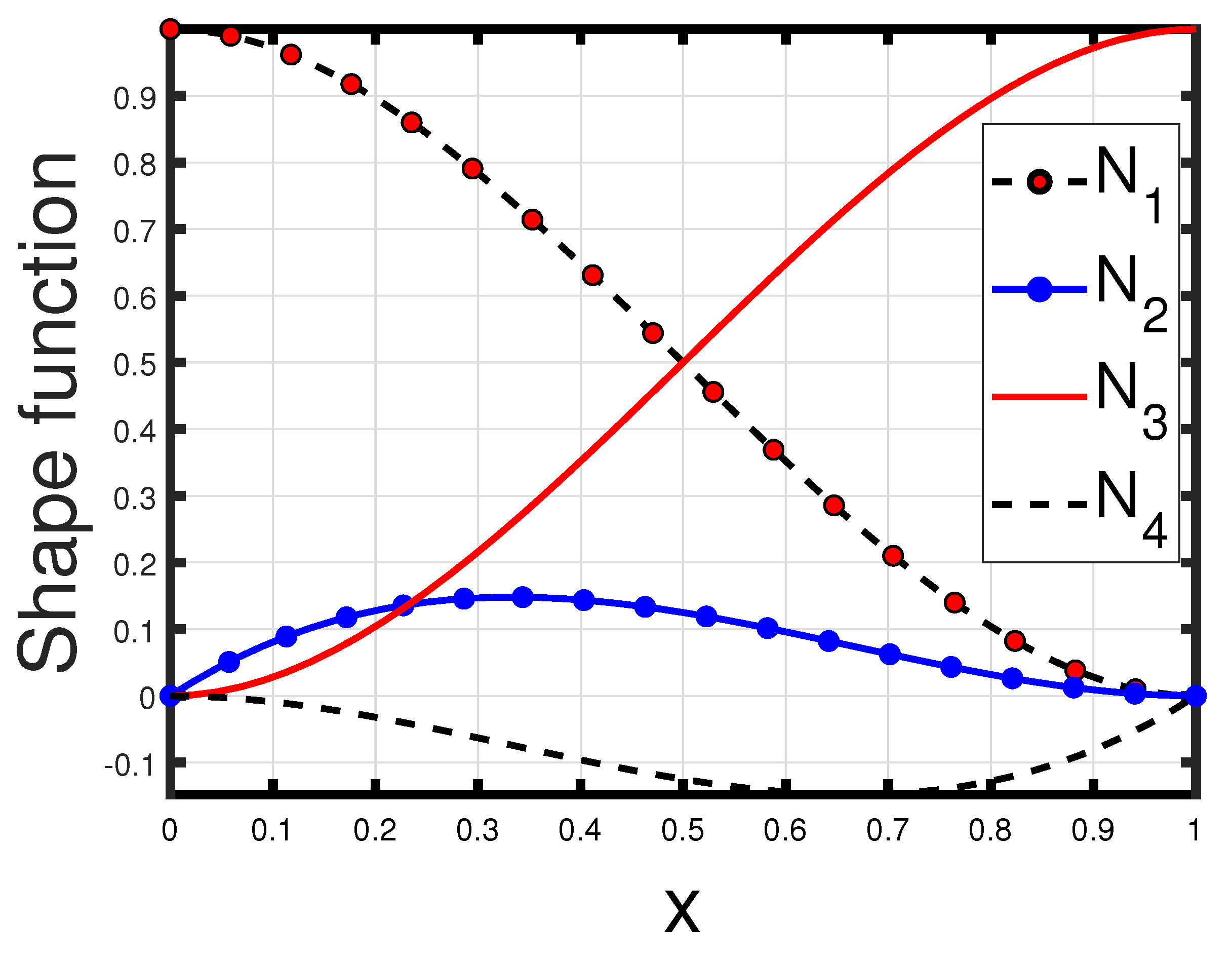
3.2. Formulation of Finite Element Method

A GFEM (Galerkin finite element method) is utilized to discretize the domain (length of the beam), which is divided into a set of finite line elements. In each beam element, there are two end nodes with two degrees of freedom each. A node can have nodal (vector) displacements or degrees of freedom, including translations (${\nu }_i;i=1,2$) and rotations $(\Psi j);j=1,2)$ as shown in Figure 2. Additionally, to obtain the differential Equation (1) in its weak form, multiply the residual by a weight function $G\left(x\right)$ and integrate by parts to evenly distribute the differentiation orders G and $\nu$. As a result, the equation is expressed as follows:

$$\begin{array}{cc}\hfill {\int }_0^{L}G& \left[EI{\nu }_{xxxx}+\rho A{\nu }_{tt}-\rho I{\nu }_{xx,tt}+K\nu (x,t)\right]dx\hfill \\ \hfill =& GEI{\nu }_{xxx}{|}_0^L-EI{\nu }_{xx}{G}_x{|}_0^L+{\int }_0^{L}EI{\nu }_{xx}{G}_{xx}dx+{\int }_0^{L}G\left[\rho A{\nu }_{tt}\right]dx\hfill \\ \hfill & -{\int }_0^{L}G\left[\rho I{\nu }_{xx,tt}\right]dx+{\int }_0^{L}GK\nu (x,t)dx=0.\hfill \end{array}$$

(28)

After determining the weak form, approximate functions are selected for each element. In the weak form, $\nu (x,t)$ has the highest third order derivative. Therefore, thrice differential approximating functions are chosen. An interpolation polynomial would meet this requirement [33]. By using GFEM, the weight function can be equated with approximate functions $G_i=N_i$, and that cubic interpolation (see in Figure 3) function can be called a cubic spline (Hermite cubic interpolation function), given as

$$N_1=1-3{\left(\frac{x}{L}\right)}^2+2{\left(\frac{x}{L}\right)}^3,N_2=x{\left(\frac{x}{L}-1\right)}^2,N_3={\left(\frac{x}{L}\right)}^2\left(3-\frac{2x}{L}\right),N_4=\frac{x^2}{L}\left(\frac{x}{L}-1\right).$$

(29)

On substituting Equation (29) into Equation (28) and $\nu :={\sum }_{j=1}^4{\nu }_{j}Nj$, we obtain

$$\begin{array}{cc}\hfill {\int }_0^{L}G& \left[EI{\nu }_{xxxx}+\rho A{\nu }_{tt}-\rho I{\nu }_{xx,tt}+K\nu (x,t)\right]dx\hfill \\ \hfill =& EI{\nu }_j{N}_i{N}_{j,xxx}{|}_0^L-EI{\nu }_j{N}_{j,xx}{N}_{i,x}{|}_0^L+{\int }_0^L(EI{N}_{i,xx}{N}_{j,xx}+K{N}_i{N}_j){\nu }_{j}dx\hfill \\ \hfill & +{\int }_0^L\left(\rho A{N}_i{N}_j-\rho I{N}_i{N}_{j,xx}\right){\nu }_{j,tt}dx=0.\hfill \end{array}$$

(30)

We can express Equation (30) as

$$\left[k_{ij}\right]{\nu }_j+\left[m_{ij}\right]{\nu }_{j,tt}=0,$$

(31)

where $k_{ij}$ and $m_{ij}$ are the stiffness and mass matrices defined as.

$$k_{ij}:={\int }_0^L(EI{N}_{i,xx}{N}_{j,xx}+K{N}_i{N}_j){\nu }_{j}dx\mathrm{and}{m}_{ij}:={\int }_0^L(\rho A{N}_i{N}_j-\rho I{N}_i{N}_{j,xx}){\nu }_{j,tt}dx.$$

where

$$k_{ij}=\left[\begin{array}{cccc}\frac{13KL}{35}+\frac{12EI}{L^3}& \frac{11K{L}^2}{210}+\frac{6EI}{L^2}& \frac{9KL}{70}-\frac{12EI}{L^3}& \frac{6EI}{L^2}-\frac{13K{L}^2}{420}\\ \frac{11K{L}^2}{210}+\frac{6EI}{L^2}& \frac{K{L}^3}{105}+\frac{4EI}{L}& \frac{13K{L}^2}{420}-\frac{6EI}{L^2}& \frac{2EI}{L}-\frac{K{L}^3}{140}\\ \frac{9KL}{70}-\frac{12EI}{L^3}& \frac{13K{L}^2}{420}-\frac{6EI}{L^2}& \frac{13KL}{35}+\frac{12EI}{L^3}& \frac{-11K{L}^2}{210}-\frac{6EI}{L^2}\\ \frac{6EI}{L^2}-\frac{13K{L}^2}{420}& \frac{2EI}{L}-\frac{K{L}^3}{140}& \frac{-11K{L}^2}{210}-\frac{6EI}{L^2}& \frac{K{L}^3}{105}+\frac{4EI}{L}\end{array}\right]$$

(32)

and

$$m_{ij}=\left[\begin{array}{cccc}\frac{13AL\rho }{35}+\frac{6I\rho }{5L}& \frac{11\rho L^2}{210}+\frac{\rho I}{10}& \frac{9AL\rho }{70}-\frac{6I\rho }{5L}& \frac{\rho I}{10}-\frac{13A{L}^2\rho }{420}\\ \frac{11A\rho L^2}{210}+\frac{\rho I}{10}& \frac{\rho A{L}^3}{105}+\frac{21\rho L}{15}& \frac{13A\rho L^2}{420}-\frac{\rho I}{10}& \frac{-\rho LI}{30}-\frac{\rho A{L}^3}{140}\\ \frac{9AL\rho }{70}-\frac{6I\rho }{5L}& \frac{13A\rho L^2}{420}-\frac{\rho I}{10}& \frac{13A\rho L}{35}+\frac{6I\rho }{5L}& \frac{-\rho I}{10}-\frac{11A{L}^2\rho }{210}\\ \frac{\rho I}{10}-\frac{13A{L}^2\rho }{420}& \frac{-\rho IL}{30}-\frac{\rho A{L}^3}{140}& \frac{-\rho I}{10}-\frac{11\rho A{L}^2}{210}& \frac{\rho A{L}^3}{105}+\frac{21\rho L}{15}\end{array}\right]$$

(33)

Therefore, if we consider harmonic time dependent ${\nu }_j$, i.e.,

$$\begin{array}{c}\hfill {\nu }_j=\left\{{\overline{\nu }}_j\right\}{e}^{i\omega t}.\end{array}$$

(34)

by substituting Equation (34) into Equation (31), we obtain

$$\left[k_{ij}\right]-{\omega }^2\left[m_{ij}\right]=0.$$

(35)

With the aid of a MATLAB code based on the GFEM, we calculate the natural frequencies and eigenmodes of beams subjected to elastic constraints. For a large number of elements, global stiffness matrices are straightforwardly produced. The Equation (35) can be utilized to determine the eigenvalues based on the stiffness and mass matrices, which further yield the eigen frequencies [31,34,35].

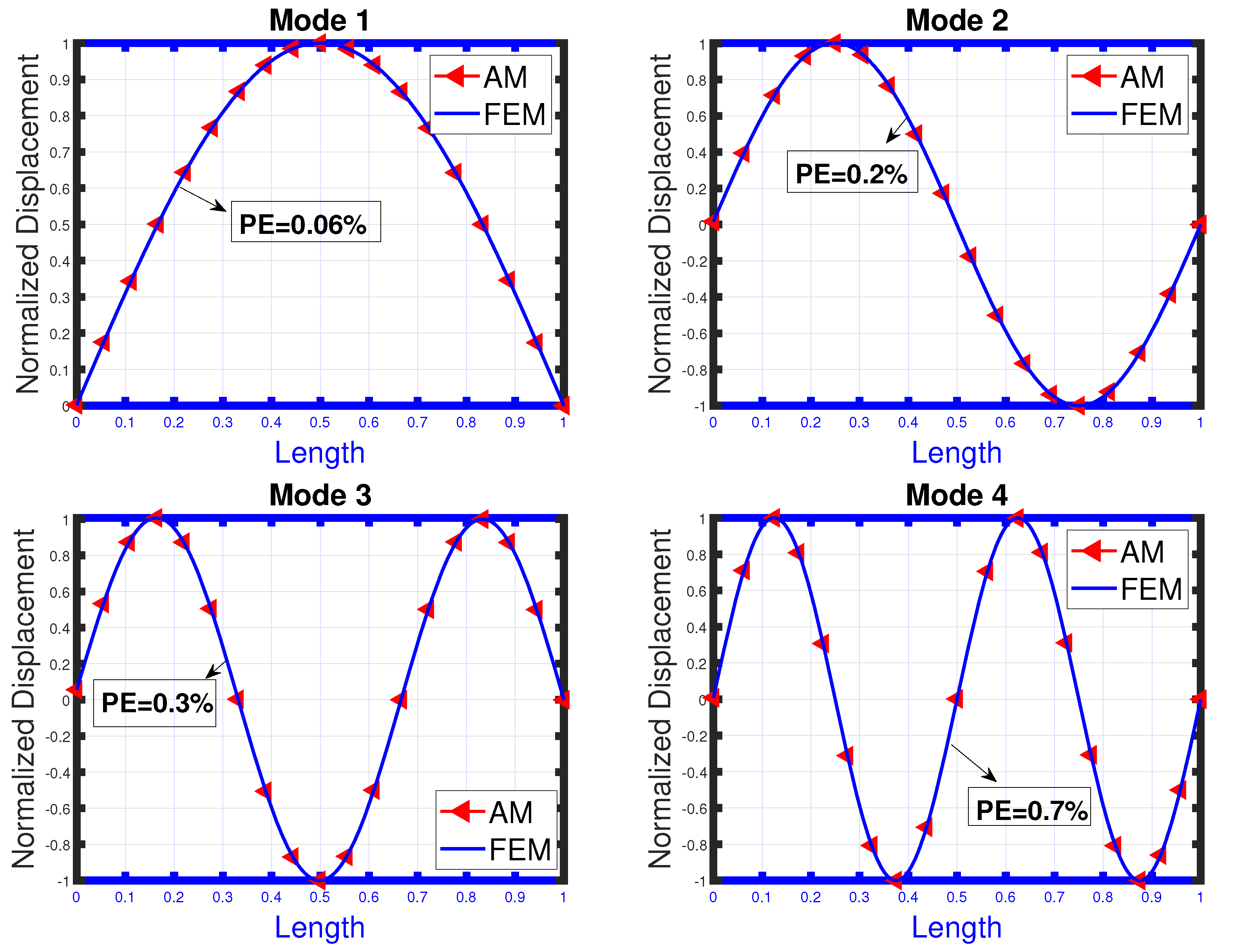
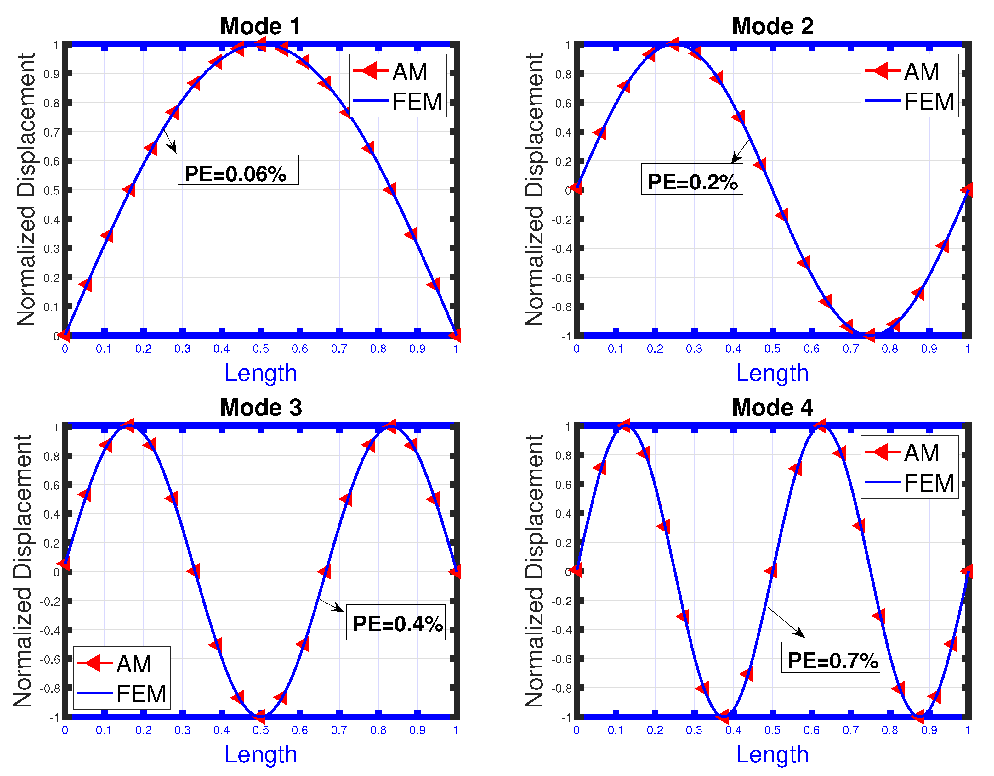
4. Results and Discussion

In this section, the proposed methods are used to determine the eigenfrequencies and eigenmodes of the elastically constrained RB and EBB with and without elastic foundation. Additionally, the frequency results of the proposed formulations are compared with the same results for the beams with classical boundary conditions available in the existing literature in order to verify its accuracy. Provided that spring parameters are given appropriate values, restrained boundary conditions degenerate into classical ones.

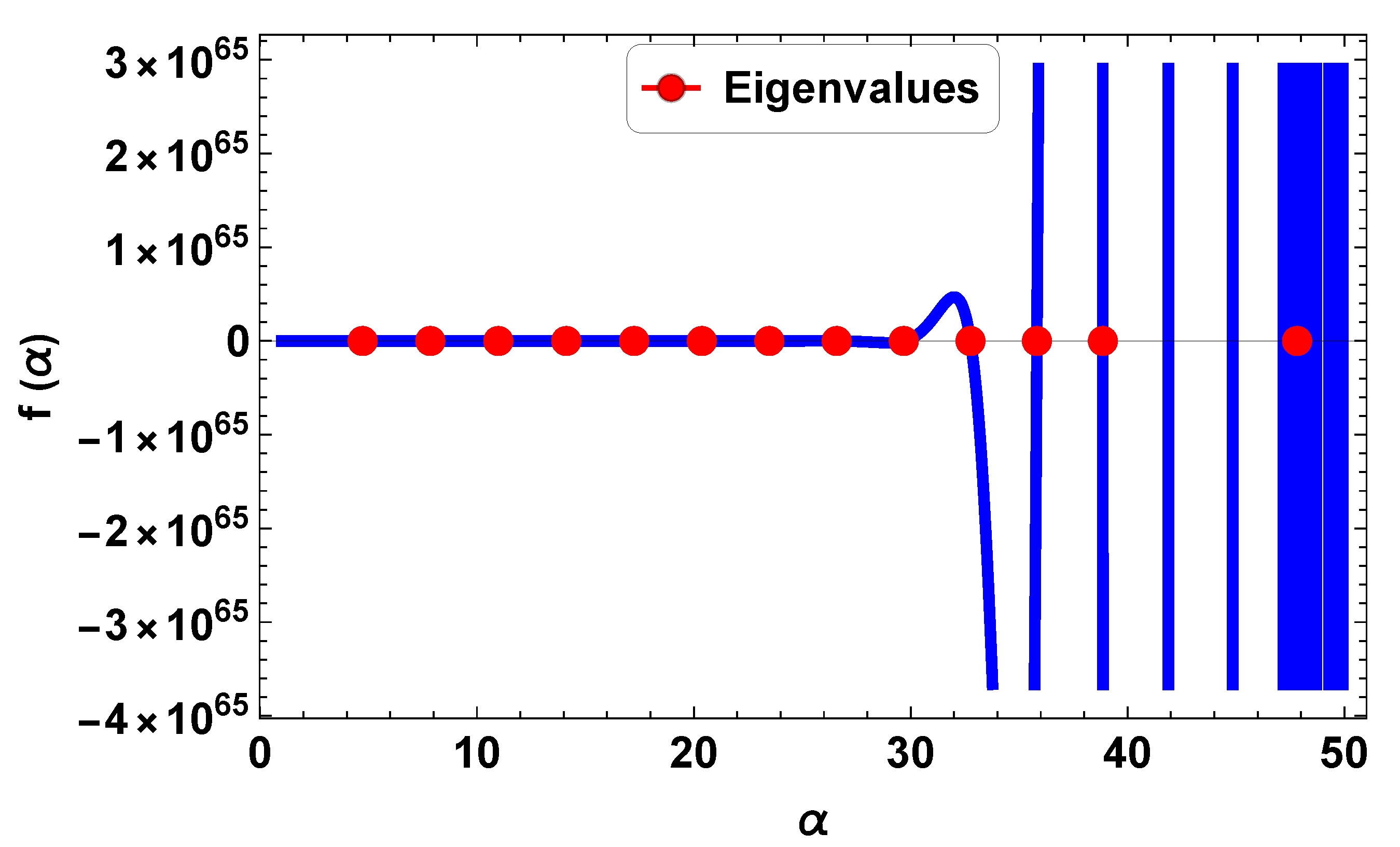
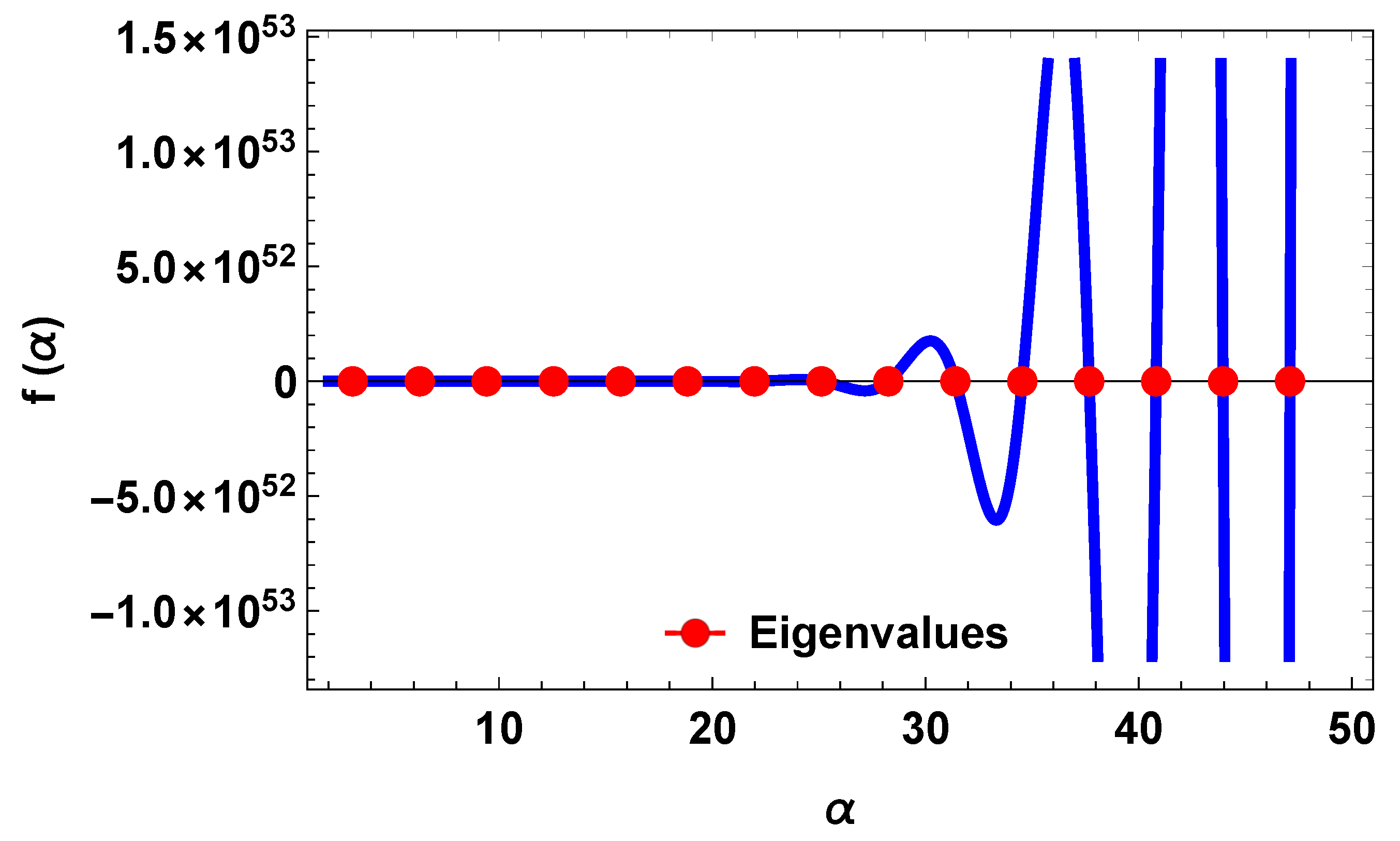
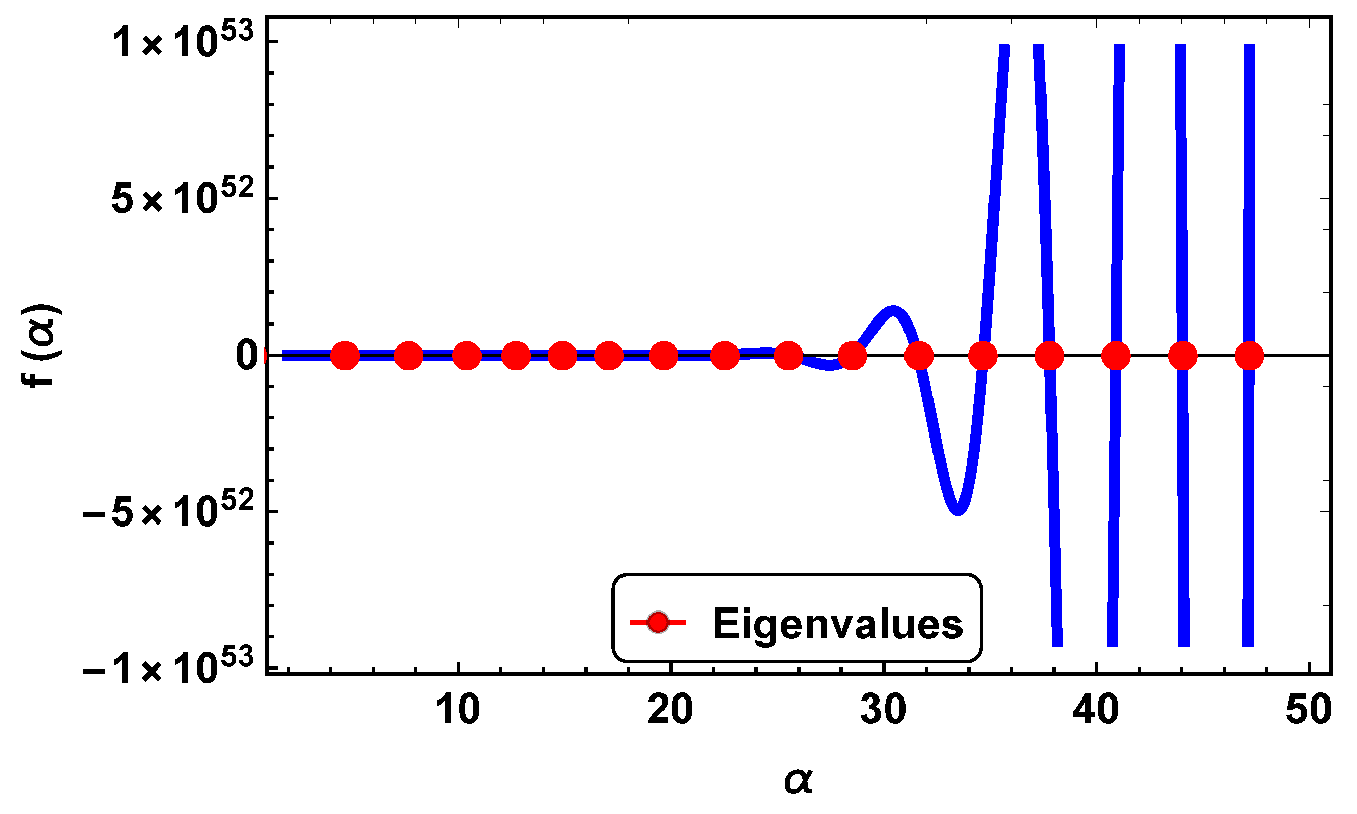
4.1. Graphical and Tabular Representations

This section presents the analysis of RB and EBB with and without Winkler elastic foundations having elastically constrained ends. The beams are made up of steel having $L=1$ m, $A=0.0075$m${}^2$, $E=207\times {10}^9$ Pa, $I=14.063\times {10}^{-6}$m${}^4$, and $\rho =76.5\times {10}^3$ kg/m${}^3$.

Figure 4, Figure 5, Figure 6 and Figure 7 depict the zeros (eigenvalues) of the dispersion relations for the RB and EBB having elastic constrained with and without elastic foundation, respectively. These eigenvalues are used to determine eigenfrequencies, which further help in determining the corresponding eigenmodes.

Table 1. The natural frequencies of the EBB and RB by varying linear and rotational springs stiffness.

BC	${\delta }_1={\delta }_2={\tau }_1={\tau }_2={10}^{12}$ (Clamped-Clamped Beam)
	${\omega }_1$	${\omega }_2$	${\omega }_3$	${\omega }_4$
RB-AM	250.696553	670.332080	1257.418531	1957.632175
RB-FEM	250.508697	668.569075	1250.974018	1952.105425
PE	0.07	0.2	0.5	0.2
EBB-FEM	253.570332	698.649266	1368.685838	2260.407107
BC	${\delta }_1={\delta }_2={\tau }_1={\tau }_2={10}^{10}$
RB-AM	244.547215	627.425812	1108.8354005	11,607.889441
RB-FEM	244.381088	626.097545	1105.006215	1600.50013598
PE	0.06	0.2	0.3	0.4
EBB-FEM	247.081229	648.3165172	1170.690514	1732.887219
BC	${\delta }_1={\delta }_2={\tau }_1={\tau }_2={10}^4$
RB-AM	0.939639	3.597750	242.763465	637.058042
RB-FEM	0.939654	3.595103	242.07727	633.471148
PE	0.01	0.07	0.2	0.5
EBB-FEM	0.9401511	3.63815	253.7942605	699.31880034
BC	${\delta }_1={\delta }_2={\tau }_1={\tau }_2={10}^2$
RB-AM	0	0.359903	242.612375	636.908474
RB-FEM	0.094067	0.359129	241.926479	633.3220740
PE	0	0.2	0.2	0.5
EBB-FEM	0.09731147	0.364811	253.638632	699.161921
BC	${\delta }_1={\delta }_2={\tau }_1={\tau }_2=0$ (Free-Free Beam)
RB-AM	0	0	242.6108484	636.906962
RB-FEM	0	0	241.924691	633.315889
PE	0	0	0.2	0.5
EBB-FEM	0	0	253.637057	699.1906165

provides a comparison of four initial modes of natural frequencies of the RB and EBB for analytical and numerical results from higher to lower values of the stiffness parameters.

It is observed that the increase in the stiffness parameter yields an increase in the natural frequency and vice versa. The highest values of the stiffness parameters provide results for clamped–clamped edges while the lowest values of stiffness parameters give results for free–free edges of the beam. The RB and EBB results show that for smaller values of the stiffness parameters, one obtains rigid body modes, i.e., the translation or rotation of the beam takes place without undergoing any significant internal deformation. The comparison of the RB and EBB show that the presence of rotatory inertia yields lesser natural frequencies for the initial four modes that are less than $1\%,3\%,5\%$, and $7\%$, respectively, than that of the EBB. Hence, the rotatory inertia impacts the higher modes of the frequencies more than the lower modes. The comparison of the analytic and numerical results in percentage error (PE) is also made. Figure 8 shows the comparison of results for the RB (by ignoring rotatory inertia) with that of the EBB for the initial four modes while keeping the stiffness parameters identical. It is observed that the results of the RB are reduced to the EBB quite accurately. Figure 9 provides the comparison of the analytical and finite element results for the RB. The graphs show excellent agreement between analytical and numerical results in the absence of an elastic foundation.

Table 2. The natural frequencies of the EBB and RB over elastic foundation for ${\delta }_1={\delta }_2={\tau }_1={\tau }_2={10}^{10}$.

K		${\mathit{\omega }}_1$	${\mathit{\omega }}_2$	${\mathit{\omega }}_3$	${\mathit{\omega }}_4$
${10}^6$	RB-AM	244.635620	627.458744	1108.853233	1607.90124959
	RB-FEM	244.469433	626.1304062	1105.023973	1600.51188801
	PE	0.06	0.2	0.3	0.4
	EBB-FEM	247.1705	648.350565	1170.709371	1732.899957
${10}^7$		245.429833	627.755057	1109.013621	1608.0075189
		245.263102	626.426070	1105.1837765	1600.617654
		0.06	0.2	0.3	0.4
		247.973024	648.656915	1170.879057	1733.01459964
${10}^8$		254.75624506	631.803299	1111.738550003	1610.2197737
		253.0629107	629.375057	1106.7805309	1601.674927
		0.6	0.3	0.4	0.5
		255.859337	651.712493	1172.574581	1734.160598
${10}^9$		321.011724	659.535432	1226.516780	1619.654366
		320.793113	658.136708	1222.621996	1612.209306
		0.06	0.2	0.3	0.4
		324.34210031	681.515201	1189.396883	1745.579210
${10}^{10}$		696.079274	890.563168	1264.837768	1711.141649
		701.049992	896.218158	1270.112079	1713.973989
		0.7	0.6	0.4	0.1
		708.897576	928.332346	1346.106578	1855.905373

presents the results of the initial four modes of the natural frequencies of the RB placed over an elastic foundation. A comparison is made between the analytic and numerical results in PE. Additionally, the results of EBB are stated for comparison purposes. According to the results, the increase in the stiffness of the elastic foundation increases the natural frequency. Moreover, this increase is relatively visible in the fundamental mode of the frequency.

Contrary to the beam that is not placed on an elastic foundation, no rigid modes are observed in this consideration. Figure 10 and Figure 11 delineate the mode shapes of the RB that is placed over an elastic foundation for different values of the stiffness parameters of attached linear and rotational springs and elastic foundation. The analytical and finite element results are compared in Figure 10, indicating a good agreement, whereas Figure 11 shows the mode shapes of the RB obtained via FEM. In contrast to an independent beam, it is noted that the RB requires a higher value of frequency to vibrate when it is placed over an elastic foundation.

Table 3. The natural frequencies of the EBB and the RB by varying rotational spring stiffness.

BC	${\delta }_1={\delta }_2={10}^9,{\tau }_1={\tau }_2={10}^{12}$
	${\omega }_1$	${\omega }_2$	${\omega }_3$	${\omega }_4$
RB-AM	247.876023	663.070974	1244.440889	1948.406590
RB-FEM	247.692291	661.344524	1238.119361	1933.149164
PE	0.07	0.2	0.5	0.7
EBB-FEM	250.685988	690.7803537	1353.424206	1933.149164
BC	${\delta }_1={\delta }_2={10}^6,{\tau }_1={\tau }_2={10}^{12}$
RB-AM	118.095539	439.042478	939.30890	1578.319082
RB-FEM	118.024116	438.040036	934.620135	1566.555535
PE	0.06	0.2	0.4	0.7
EBB-FEM	119.183343	454.989152	1014.407906	1796.176890
BC	${\delta }_1={\delta }_2={10}^3,{\tau }_1={\tau }_2={10}^{12}$
RB-AM	110.868207	431.774070	931.988756	1571.619022
RB-FEM	110.801167	430.788243	927.610823	1559.904574
PE	0.06	0.2	0.4	0.7
EBB-FEM	111.889149	447.456074	1006.476980	1788.564665
BC	${\delta }_1={\delta }_2=0,{\tau }_1={\tau }_2={10}^{12}$ (Supported-Supported beam)
RB-AM	110.860491	431.766562	931.981563	1571.612216
RB-FEM	110.793383	430.779004	927.586263	1559.814971
[31]	110.867126	431.85454	932.340065	—–
PE	0.06	0.2	0.3	0.7
EBB-FEM	111.881330	447.448294	1006.469162	1788.556629
[31]	111.888296	447.553217	1006.994779	—–

,

Table 4. The natural frequencies of the EBB and RB over elastic foundation for ${\delta }_1={\delta }_2={10}^3$, ${\tau }_1={\tau }_2={10}^{12}$.

K		${\mathit{\omega }}_1$	${\mathit{\omega }}_2$	${\mathit{\omega }}_3$	${\mathit{\omega }}_4$
${10}^6$	RB-AM	111.073523	431.8216718	932.009064	1571.629866
	RB-FEM	110.996365	430.835737	927.631036	1559.915337
	PE	0.06	0.2	0.4	0.7
	EBB-FEM	112.086260	447.505404	1006.498912	1788.577007
${10}^7$		112.562480	432.249847	932.191820	1571.727457
		112.737932	431.262934	927.812933	1560.012200
		0.1	0.2	0.2	0.7
		113.844930	447.794913	1006.696279	1778.688080
${10}^8$		128.943498	436.508501	934.017415	1572.703052
		128.865529	435.512864	929.629948	1560.980497
		0.06	0.2	0.4	0.7
		130.120866	452.362476	1008.667823	1789.798432
${10}^9$		235.877972	477.008461	952.080831	1582.425719
		235.735339	475.919341	947.608469	1570.630622
		0.06	0.2	0.4	0.7
		238.735339	494.333492	1028.175362	1800.864299
${10}^{10}$		667.650974	772.987265	1116.758071	1676.553113
		667.247203	771.222161	1111.511651	1664.055472
		0.06	0.2	0.4	0.7
		673.799540	801.064028	1206.019299	1907.996384

and

Table 5. The natural frequencies of the EBB and RB by varying linear spring stiffness.

BC	${\delta }_1={\delta }_2={10}^{10},{\tau }_1={\tau }_2={10}^4$
	${\omega }_1$	${\omega }_2$	${\omega }_3$	${\omega }_4$
RB-AM	0.939662	110.809968	431.603421	931.7944980
RB-FEM	0.939663	110.742948	430.617197	927.411308
PE	0.001	0.6	0.2	0.4
EBB-FEM	0.939852	111.8306027	447.292920	100.640580
BC	${\delta }_1={\delta }_2={10}^{10},{\tau }_1={\tau }_2={10}^3$
RB-AM	0.297149	110.802923	431.601704	931.794248
RB-FEM	0.297230	110.735907	430.615483	927.410579
PE	0.02	0.06	0.2	0.4
EBB-FEM	0.297394	111.823493	447.2291140	100.640501
BC	${\delta }_1={\delta }_2={10}^{10},{\tau }_1={\tau }_2={10}^2$
RB-AM	0.0939667	110.802218	431.601533	931.794167
RB-FEM	0.093957	110.735202	430.615312	927.410506
PE	0.01	0.06	0.2	0.4
EBB-FEM	0.098001	111.822788	447.290962	100.640493
BC	${\delta }_1={\delta }_2={10}^{10},{\tau }_1={\tau }_2=10$
RB-AM	0.0297149	110.802148	431.601515	931.794167
RB-FEM	0.029710	110.735133	430.615295	927.410498
PE	0.01	0.06	0.2	0.4
EBB-FEM	0.033645	111.822711	447.290944	100.640493
BC	${\delta }_1={\delta }_2={10}^{10},{\tau }_1={\tau }_2=0$
RB-AM	0	110.802140	431.601513	931.794166
RB-FEM	0.001565	110.735124	430.615293	927.410498
PE	0	0.06	0.2	0.4
EBB-FEM	0.033058	111.8227109	447.290943	100.640493

furnish the comparison of analytical and finite element results for varying the stiffness of rotational spring, elastic foundation, and linear spring, respectively. A decrease is observed in the natural frequency in each of the modes when one of the stiffness parameters is decreased and the other(s) is/are fixed. However, the fundamental frequency is considerably reduced as compared to higher modes frequencies.

Based on the analysis conducted, it can be deduced that manipulating the elastic foundation parameter allows for the adjustment of the vibrating frequency, thereby minimizing the duration for potential collateral damage to the vibrating structure. Consequently, placing the beam on an elastic foundation serves as a means to regulate its vibration and mitigate the risk of structural damage.

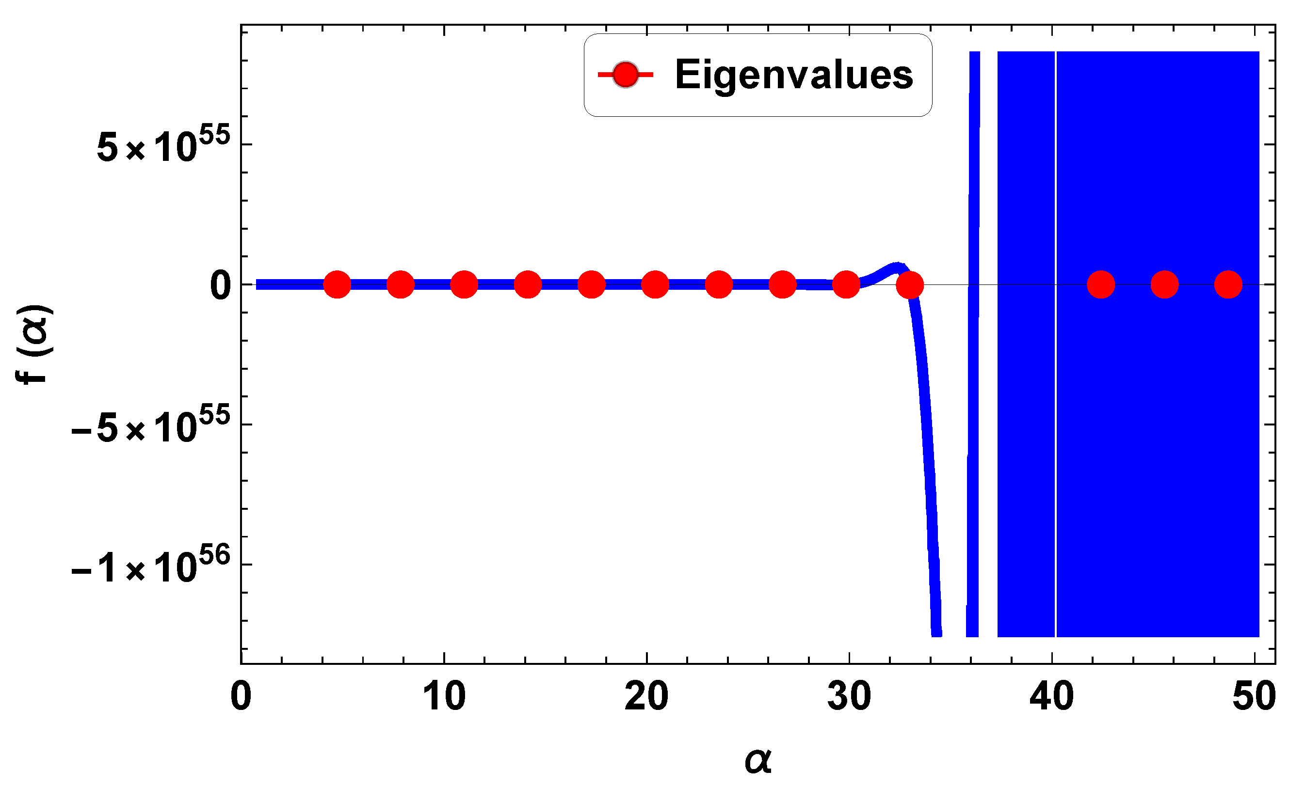
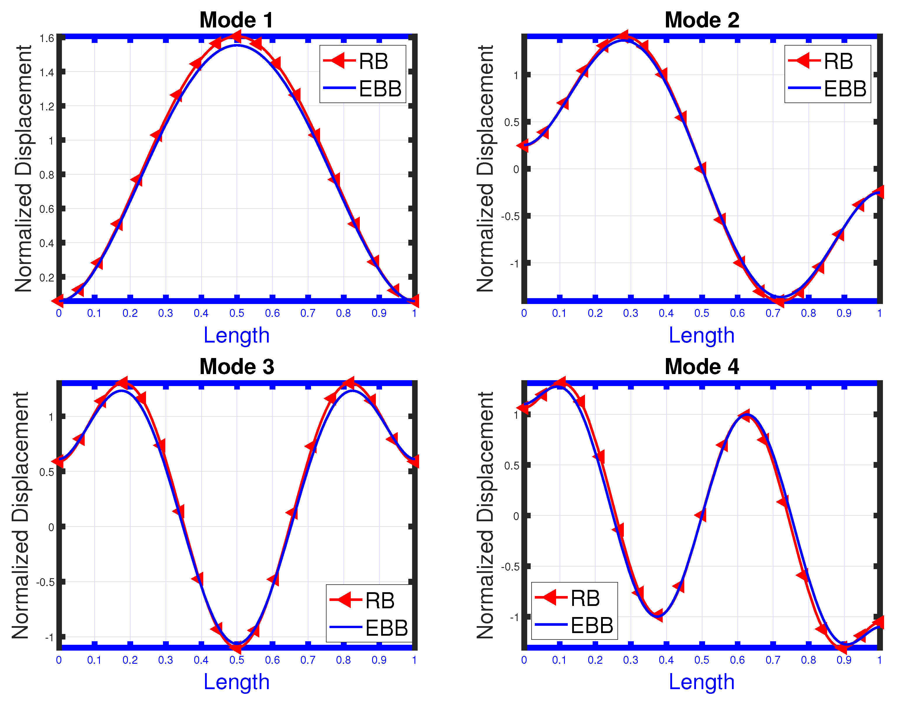
4.2. Validation of the Results

This subsection aims to provide the validity of the results obtained above. For this purpose, the underlying results are rendered for some special cases already reported in the literature. Rao [31] has outlined the natural frequencies of supported–supported RB and EBB by considering $L=1$ m, $A=0.0075$ m${}^2$, $E=207\times {10}^9$ Pa, $I=14.063\times {10}^{-6}$ m${}^4$, and $\rho =76.5\times {10}^3$ kg/m${}^3$, respectively. If the stiffness parameters of the linear and rotational springs are taken as ${\tau }_1={\tau }_2={10}^{12}$ and ${\delta }_1={\delta }_2=0$, respectively, then the results obtained by Rao [31] are verified for simply supported edges. Additionally, the results of the EBB [36] and the RB for clamped–clamped edges are verified by letting the stiffness parameters as ${\tau }_1={\tau }_2={\delta }_1={\delta }_2={10}^{12}$. It is further observed that by equating the stiffness parameters of linear and rotational springs to zero, the obtained results are verified with that of free–free Euler–Bernoulli beam [36].

5. Conclusions

The frequency analysis of a beam resting on an elastic foundation and subject to rotary inertia effects has been studied. Analytical and finite element schemes have been used to determine the natural frequencies and corresponding mode shapes of the vibrating beam. The results have been obtained for the Rayleigh beam subjected to rotational and linear springs while the results for Euler–Bernoulli have been reduced as special cases. The key findings of the analysis are given as:

• The eigenvalues obtained in terms of the slenderness ratio for the RB depend on the geometry, unlike the EBB where eigenvalues do not depend on the slenderness ratio.
• The behavior of a beam under different conditions, such as the presence of rotatory inertia or placement on an elastic foundation, impacts its natural frequencies.
• For smaller stiffness parameters, the beam undergoes rigid body modes without significant internal deformation.
• The inclusion of rotational inertia had a minimal effect on the fundamental mode frequency, but it had a significant impact on the higher frequency modes.
• Placing the Winkler elastic foundation under the beam caused an increase in stiffness, leading to higher frequencies as the elastic foundation stiffness increased.
• A detailed tabular and graphical analysis proved that the vibration frequencies and mode shapes are more affected by the linear spring stiffness compared to rotary spring stiffness.
• Unlike independent beams, beams on an elastic foundation require higher frequencies to vibrate. Thus, by controlling the elastic foundation parameter, one can adjust the vibrating frequency to minimize collateral damage to the vibrating structure.
• While comparing results with the existing ones in the literature, it has been observed that the finite element scheme provided the best accuracy for obtaining the mode shapes of the beam structure.

Therefore, it is concluded that the more complex nature of the beam structures can be treated with the numerical scheme established here. Optimal solutions for beams resting on multi-parameter foundations containing simultaneous shear deformation and rotational effects can be calculated considering forced vibration and dynamical boundary conditions. The strength of this study lies in the fact that its implications may lead to the development of more accurate and efficient numerical methods for analyzing beam structures, which can be used in building construction to provide essential support and stability to the structure. The findings may also be useful in designing beams that can minimize collateral damage to the vibrating structure by controlling the elastic foundation parameter. The research article may also pave the way for further research into the behavior of beams under different conditions, such as the presence of rotatory inertia or placement on an elastic foundation, and the impact on their natural frequencies. Contrarily, while the article provides detailed analysis and numerical methods for the vibrational frequencies of the Rayleigh beam, it is limited in terms of practical applications as it does not provide any experimental validation of the results.

References

1. Chun, K.R. Free vibration of a beam with one end spring-hinged and the other free. J. Appl. Mech. 1972, 39, 1154–1155. [Google Scholar] [CrossRef]
2. Lee, T.W. Vibration frequencies for a uniform beam with one end spring-hinged and carrying a mass at the other free end. J. Appl. Mech. 1973, 40, 813–815. [Google Scholar] [CrossRef]
3. Lai, H.Y.; Hsu, J.C. An innovative eigenvalue problem solver for free vibration of Euler-Bernoulli beam by using the Adomian decomposition method. Comput. Math. Appl. 2008, 56, 3204–3220. [Google Scholar] [CrossRef] [Green Version]
4. Smith, R.C.; Bowers, K.L.; Lund, J. A fully sinc-Galerkin method for Euler-Bernoulli beam models. Numer. Methods Partial. Differ. Equ. 1992, 8, 171–202. [Google Scholar] [CrossRef] [Green Version]
5. Hess, M.S. Vibration frequencies for a uniform beam with central mass and elastic supports. J. Appl. Mech. 1964, 31, 556–557. [Google Scholar] [CrossRef]
6. Grossi, R.O.; Arenas, B. A variational approach to the vibration of tapered beams with elastically restrained ends. J. Sound Vib. 1996, 195, 507–511. [Google Scholar] [CrossRef]
7. Naguleswaran, S. Transverse vibration of a uniform Euler-Bernoulli beam under linearly varying axial force. J. Sound Vib. 2004, 275, 47–57. [Google Scholar] [CrossRef]
8. Naguleswaran, S. Natural frequencies, sensitivity, and mode shape details of an Euler-Bernoulli beam with one-step change in cross-section and with ends on classical supports. J. Sound Vib. 2002, 252, 751–767. [Google Scholar] [CrossRef]
9. Laura, P.A.A.; De Irassar, P.V.; Ficcadenti, G.M. A note on transverse vibrations of continuous beams subject to an axial force and carrying concentrated masses. J. Sound Vib. 1983, 86, 279–284. [Google Scholar] [CrossRef]
10. Abbas, B.A.H. Vibrations of Timoshenko beams with elastically restrained ends. J. Sound Vib. 1984, 97, 541–548. [Google Scholar] [CrossRef]
11. Rao, G.V.; Naidu, N.R. Free vibration and stability behavior of uniform beams and columns with non-linear elastic end rotational restraints. J. Sound Vib. 1994, 176, 130–135. [Google Scholar] [CrossRef]
12. Civalek, Ö. Application of differential quadrature (DQ) and harmonic differential quadrature (HDQ) for buckling analysis of thin isotropic plates and elastic columns. Eng. Struct. 2004, 26, 171–186. [Google Scholar] [CrossRef]
13. Kim, H.K.; Kim, M.S. Vibration of beams with generally restrained boundary conditions using Fourier series. J. Sound Vib. 2001, 245, 771–784. [Google Scholar] [CrossRef]
14. Mahapatra, K.; Panigrahi, S.K. Dynamic Response of a Damped Euler–Bernoulli Beam Having Elastically Restrained Boundary Supports. J. Inst. Eng. (India) Ser. C 2019, 100, 891–905. [Google Scholar] [CrossRef]
15. Villa-Morales, J.; Rodríguez-Esparza, L.J.; Ramírez-Aranda, M. Deflection of Beams Modeled by Fractional Differential Equations. Fractal Fract. 2022, 6, 626. [Google Scholar] [CrossRef]
16. Zhao, X.; Chang, P. Free and forced vibration of a double beam with arbitrary end conditions connected with a viscoelastic layer and discrete points. Int. J. Mech. Sci. 2021, 209, 106707. [Google Scholar] [CrossRef]
17. Wang, J.I. Vibration of stepped beams on elastic foundations. J. Sound Vib. 1991, 149, 315–322. [Google Scholar] [CrossRef]
18. Lai, Y.C.; Ting, B.Y.; Lee, W.S.; Becker, B.R. Dynamic response of beams on elastic foundation. J. Struct. Eng. 1992, 118, 853–858. [Google Scholar] [CrossRef]
19. Thambiratnam, D.; Zhuge, Y. Free vibration analysis of beams on elastic foundation. Compos. Struct. 1996, 60, 971–980. [Google Scholar] [CrossRef]
20. Gülkan, P.; Alemdar, B.N. Two-parameter elastic foundation: A revisit. Struct. Eng. Mech. 1999, 7, 259–276. [Google Scholar] [CrossRef]
21. Al-Hosani, K.; Fadhil, S.; El-Zafrany, A. Fundamental solution and boundary element analysis of thick plates on Winkler foundation. Comput. Struct. 1999, 70, 325–336. [Google Scholar] [CrossRef]
22. Yayli, M.Ö.; Aras, M.; Aksoy, S. An efficient analytical method for vibration analysis of a beam on an elastic foundation with elastically restrained ends. Shock Vib. 2014, 2014, 159213. [Google Scholar] [CrossRef] [Green Version]
23. Nawaz, R.; Nuruddeen, R.I.; Zia, Q.M. An asymptotic investigation of the dynamic and dispersion of an elastic five-layered plate for anti-plane shear vibration. J. Eng. Math. 2021, 128, 1–12. [Google Scholar] [CrossRef]
24. Asif, M.; Nawaz, R.; Nuruddeen, R.I. Dispersion of elastic waves in an inhomogeneous multilayered plate over a Winkler elastic foundation with imperfect interfacial conditions. Phys. Scr. 2021, 96, 125026. [Google Scholar] [CrossRef]
25. Doeva, O.; Masjedi, P.K.; Weaver, P.M. Static analysis of composite beams on variable stiffness elastic foundations by the Homotopy Analysis Method. Acta Mech. 2021, 232, 4169–4188. [Google Scholar] [CrossRef]
26. Zhiyuan, L.; Yepeng, X.; Dan, H. Analytical solution for vibration of functionally graded beams with variable cross-sections resting on Pasternak elastic foundations. Int. J. Mech. Sci. 2021, 191, 106084. [Google Scholar]
27. Mirzabeigy, A.; Madoliat, R.; Vahabi, M. Free vibration analysis of two parallel beams connected together through variable stiffness elastic layer with elastically restrained ends. Adv. Struct. Eng. 2017, 20, 275–287. [Google Scholar] [CrossRef]
28. Njim, E.K.; Muhannad, A.W.; Sadeq, H.B. A Critical Review of Recent Research of Free Vibration and Stability of Functionally Graded Materials of Sandwich Plate. IOP Conf. Ser. Mater. Sci. Eng. 2021, 1094, 012081. [Google Scholar] [CrossRef]
29. Sheng, G.G.; Wang, X. The dynamic stability and nonlinear vibration analysis of stiffened functionally graded cylindrical shells. Appl. Math. Model. 2018, 56, 389–403. [Google Scholar] [CrossRef]
30. Valipour, P.; Ghasemi, S.E.; Khosravani, M.R.; Ganji, D.D. Theoretical analysis on nonlinear vibration of fluid flow in single-walled carbon nanotube. J. Theor. Appl. Phys. 2016, 10, 211–218. [Google Scholar] [CrossRef] [Green Version]
31. Rao, S.S. Vibration of Continuous Systems; John Wiley and Sons: Hoboken, NJ, USA, 2007; ISBN 978-0-471-77171-5. [Google Scholar]
32. Han, S.M.; Benaroya, H.; Wei, T. Dynamics of transversely vibrating beams using four engineering theories. J. Sound Vib. 1999, 225, 935–988. [Google Scholar] [CrossRef] [Green Version]
33. Ferreira, A.J.M. MATLAB Codes for Finite Element Analysis: Solids and Structures; Solid Mechanics and Its Applications 157; Springer: Berlin/Heidelberg, Germany, 2009. [Google Scholar]
34. Kreyszig, E. Advanced Engineering Mathematics, 10th ed.; John Wiley and Sons: Hoboken, NJ, USA, 2009. [Google Scholar]
35. Meirovitch, L. Fundamentals of Vibrations (Long Grove); McGraw-Hill Education: New York, NY, USA, 2001. [Google Scholar]
36. Leissa, A.W.; Qatu, M.S. Vibrations of Continuous Systems; McGraw-Hill Education: New York, NY, USA, 2011. [Google Scholar]
Figure 1. Beam configuration: Rayleigh beam resting on an elastic foundation with elastic constraints.
Buildings 13 01457 g001
Figure 2. A beam element.
Buildings 13 01457 g002
Figure 3. Shape function for RB.
Buildings 13 01457 g003
Figure 4. Eigenvalues of the EBB without elastic foundation by letting δ 1 = δ 2 = τ 1 = τ 2 = 10 4 .
Buildings 13 01457 g004
Figure 5. Eigenvalues of the EBB with elastic foundation by letting δ 1 = δ 2 = τ 1 = τ 2 = 10 12 , and K = 10 10 . .
Buildings 13 01457 g005
Figure 6. Eigenvalues of the RB without elastic foundation by letting δ 1 = δ 2 = 10 10 , τ 1 = τ 2 = 10 2 .
Buildings 13 01457 g006
Figure 7. Eigenvalues of the RB with elastic foundation by letting δ 1 = δ 2 = τ 1 = τ 2 = 10 10 , and K = 10 8 .
Buildings 13 01457 g007
Figure 8. The first four lowest mode shapes of the RB and EBB for δ 1 = δ 2 = τ 1 = τ 2 = 10 10 .
Buildings 13 01457 g008
Figure 9. The first four lowest mode shapes of the RB for δ 1 = δ 2 = 0 and τ 1 = τ 2 = 10 12 .
Buildings 13 01457 g009
Figure 10. The first four lowest eigenmodes of the RB over elastic foundation for δ 1 = δ 2 = 10 3 , τ 1 = τ 2 = 10 12 , and K = 10 8 .
Buildings 13 01457 g010
Figure 11. The first four lowest mode shapes of the RB resting over elastic foundation for δ 1 = δ 2 = τ 1 = τ 2 = 10 10 and K = 10 9 .
Buildings 13 01457 g011