Abstract
The LIFE-funded European research project SUBproducts4LIFE seeks to demonstrate the use of industrial subproducts for the large-scale remediation of contaminated soils and industrial building debris connected to Hg mining. The main purpose of the present research was to ensure worker health and safety by creating a protocol for working in a highly mercury-contaminated demolition debris. A methodology consisting of sampling campaigns with a Lumex RA-915 mercury analyser, evaluating the accuracy of an empirical Hg emission model, evaluating each working task, providing recommendations for minimising the workers’ exposure and calculating the maximum work period in each area was proposed. It was also shown to forecast Hg biological markers. As a result, a work protocol was developed with three scenarios which allow planning the work and forecasting the workers’ mercury exposure as a function of the daily temperature, ensuring that the workers’ mercury exposure is below occupational mercury levels. The working protocol allows planning the works safely with minimum exposure to gaseous mercury and working fulfilling standard requirements. Plans for restoration or new use of industrial mercury-contaminated sites have increased in recent years, and the research improves the knowledge of Hg gas distribution and worker Hg exposure.
1. Introduction
Mercury has been a well-known metal since ancient times; in the past 500 years, 992,812 tons of mercury have been produced worldwide [1], with the most significant producers being Spain, the USA, Slovenia, and Italy. Since 1971, the use of mercury has been declining, and it is now prohibited in many countries. However, certain nations still produce mercury, including China, Tajikistan, and Mexico, and in other cases, mercury is produced as a subproduct. In most cases, mercury mining facilities were abandoned without any intentions for restoration, similar to other mercury-related buildings such as mercury chlor-alkali plants [2], scrap metal processing facilities [3], copper and zinc smelting factories, and weapon production buildings [4] generating tons of hazardous waste which nowadays is a significant public health issue. There are plans to decommissioning these facilities, and it is crucial to ensure the health and safety of the workers and all the people involved. This research evaluates the working conditions in heavily mercury-contaminated facilities.
1.1. Brief State of the Art
Heavy metal contamination in buildings is a major environmental problem threatening public health. Because of the issue’s importance, this topic has been thoroughly researched in the scientific literature. Several categories can be used for group research. The preservation of the environment comes first. Understanding mercury gas emissions from places with high mercury concentrations has advanced significantly in the recent decades, e.g., Wang et al. [5]; Gustin [6]; Feng et al. [7] demonstrated in their findings that the Hg gas emission rates from mercury-enriched soils are significantly higher than the values observed in the background area and that the amount of gaseous mercury contributed by Hg-enriched soil in the mercuriferous belt to the atmosphere has been substantially underestimated [6,7]. As a result, many topics have been thoroughly studied, such as the concentration of mercury (Hg) in the soil and water near contaminated sites [8,9,10], as well as the rates of emission into the atmosphere and the distribution of the contamination around the sites affected by mercury mining [5,11,12,13,14,15,16].
Another area of study is the creation of emission models, such as those by Lindberg et al. [17] and Llanos et al. [18], which aid in analysing potential dangers associated with Hg pollution. Matanzas et al. [19] have conducted other particular investigations, such as the transfer of Hg to plants.
The impact of pollution on human health is a different area of study [20]. Both broad investigations, such as those by Kim et al. [21] and Wu et al. [22], and more focused ones, such as those by Phelps et al. [23] or Koeningsmark [24], have been conducted. The World Health Organization (WHO) states that breathing in mercury can have catastrophic consequences for the lungs, kidneys, and immunological, neurological, and digestive systems. Memory loss, neuromuscular effects, headaches, cognitive and motor problems, tremors, and insomnia are a few adverse effects of the exposure. When mercury is present in exceptionally high amounts, it has been demonstrated to produce a variety of malignancies in rats and mice [25,26]. The most poisonous forms of mercury are methylmercury and metallic mercury vapour, which can irreversibly damage the kidneys, the developing foetus, and the brain at large doses. Other effects of mercury include diminished fertility, abdominal pain, inflammatory bowel disease, ulcers, bloody diarrhoea, and intestinal flora loss. The liver, brain, and kidneys are the body’s primary locations for mercury bioaccumulation [27].
The commerce and use of mercury are currently prohibited under the Minamata Convention on Mercury. Some traditional products have disappeared, such as mercury-based measurement equipment (thermometers, barometers and sphygmomanometers), light bulbs, neon sign producers, etc. On the contrary, the production has increased in other industries where workers can be exposed to mercury, such as waste and recycling or companies involved with contaminated land and bioremediation. Attempts to diminish the risk of worker exposure to mercury have made the Hg levels in workers’ urine in the UK decrease from 90% (P90) of 24.7 µmol/mol creatinine in 1997 to 2.1 µmol/mol creatinine in 2019, as it has been studied by Morton et al. [28].
The remediation of contaminated sites and specifically the occupational dangers of working in these locations are the subject of another category of research. Despite the subject’s significance, there are not many studies in this area. However, there have been recent studies that are pretty pertinent; for instance, Wcislo et al. [29] evaluated the human health risk assessment in restoring safe and beneficial use of contaminated areas that have been abandoned. There are some studies about biological parameters such as the level of Hg in blood, urine or hair [30,31,32]. The assessment and clean-up of mercury-contaminated sites and human and ecological Hg exposure and risk are covered in depth by Eckley et al. [33]. Due to the complexity of the pollution situations, González-Valoys et al. [34] suggest risk evaluations of an abandoned gold mine in Panama using combinations of indices. There is also some research on managing hazardous mercury waste [4].
Similarly, Wcislo et al. [35] assess the health risk of working in post-mining HgAs-contaminated soils. Other studies, including those by Wongsasuluk et al. [36], analyse the health risks associated with exposure to heavy metals such as arsenic in operating mines. This latter class may incorporate the current piece of work.
1.2. SUBproducts4LIFE Project
A research project called SUBproducts4LIFE is being co-funded by the European Union as a part of the LIFE initiative. By reusing industrial waste (coal ash, gypsum, blast furnace slag, and steelmaking slag) to restore polluted soils, brownfield sites and building debris connected to Hg mining in the decommissioned site of La Soterraña, the initiative seeks to demonstrate cutting-edge circular economy concepts (Figure 1).
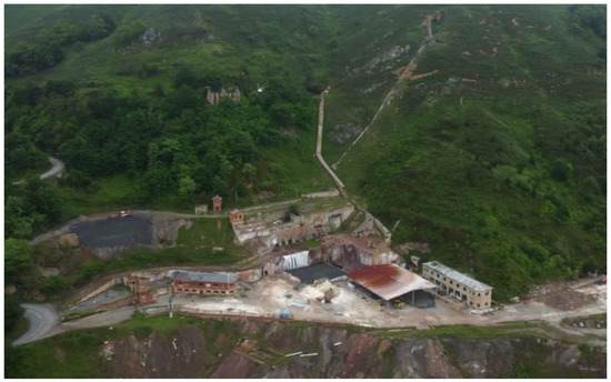
Figure 1.
Facilities of the decommissioned Hg mine, La Soterraña [37].
One of the project’s goals is to ensure the safety of the workers by creating guidelines and a manual of best practices for working in these highly hazardous locations.
This study is the continuation of the previous studies on the characterisation of Hg contamination in the air:
Preliminary analysis by Garcia-Gonzalez et al. [25] was conducted, in which it was demonstrated that particle concentrations of As and Hg in the air were minimal.
Then, an empirical model was developed to predict the Hg gaseous concentration emissions at any temperature in highly contaminated areas (Rodríguez et al. [38]).
Finally, a chemical–physical model to explain the emission and diffusion of Hg at a short distance from the metallurgical plant demolition was established by Rodríguez et al. [39].
1.3. Empirical Model: Description, Planning, Risk Assessment
The starting point of the present work is the emission and diffusion empirical models determined previously. It is based on the solid relationship between emissions and soil temperature, as stated by Scholtz et al. [11] (referencing Siegel and Siegel [40], Zhang et al. [41] and Lindberg et al. [17]). Mercury concentration measurements were carried out under different climatic conditions (temperatures between 4 °C and 30 °C and without rain or wind) to evaluate the influence of temperature on the potential release of Hg in the area with demolition debris from the metallurgical plant building. All the measurements were carried out at 1.0–1.5 m above ground level because it is the recommended height for airborne pollution environmental values [42]. Figure 2A displays these values and shows that the correlation between temperature θ (°C) and concentration over debris area C10 (ng/m3) can be explained well by Equation (1) [38].
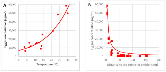
Figure 2.
Relationship between temperature and concentration at point 10 (A) and concentration variation with the distance to the focus for θ = 25–30 °C (B).
As previously mentioned, measurements were also performed at various distances from the centre of the focus. Radial diffusion can explain the existence of gaseous mercury as we move away from the source of contamination. This diffusion follows a hyperbolic curve that varies inversely with distance from the source. Figure 2B represents Hg concentration between 24 °C and 30 °C. Therefore, according to the following Equation (2), also established empirically, the fluctuation of the concentration varies with the distance to the focus of the contamination:
1.4. Objectives of the Study
The principal purpose of the research is to evaluate the work managing demolition waste highly contaminated with mercury in terms of gaseous mercury in the environment and to design a plan for health and safety at work. The steps taken to achieve this objective are the following:
- A gaseous Hg measurement campaign was carried out in the area, with a sampling period of 2 hours following the EN-689:2018 standard [43]. The workplace was differentiated based on the Hg gas concentration in the environment. The accuracy of the empirical model proposed in previous work was verified, and it was shown that temperature is the crucial variable.
- A risk prevention criterion for exposure to gaseous Hg was defined following EN-689:2018, which limits working hours in the most contaminated areas based on ambient temperature; based on it, a protocol was developed to work in health and safety conditions for workers. On the other hand, it is stated that covering the contaminated material is an effective safety measure for worker protection.
- Analysis of the actual work completed was conducted, detailing the actual activities in the riskiest areas (something that is not typically published in the specialised bibliography); based on the empirical model and the risk prevention criterion, an appropriate way to respond was defined, first during the planning of the tasks, and then during their execution, so that the quality standards in terms of health and safety are met at all times.
2. Materials and Methods
2.1. Measuring Device and Sampling Procedure
The LUMEX RA-915 sampling device had an analytical gaseous Hg range of 1–100,000 ng/m3 (Figure 3, left). The instrument collected 10 litres of air every minute and recorded the data in an internal data logger while reporting analysis every second as well as the 10 s average. This instrument is widely used in scientific research and by reference organisations to measure gaseous mercury in various circumstances and conditions. Mercury particles removed via a filter at the equipment’s inlet are not included in the LUMEX RA-915’s analysis of gaseous mercury.
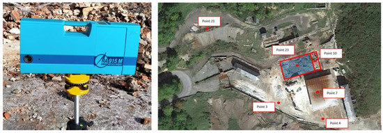
Figure 3.
The Lumex analyser (left) and areas represented by points 10 and 23 (right).
In order to create work protocols, a sample procedure was designed; sampling locations and systematic monitoring campaigns were planned. A route with 22 control stations spread out along the area where the Hg gas concentrations were measured under various circumstances to establish the empirical model. Nevertheless, this study only monitored the points at which work was carried out. The study’s main objective is to evaluate the location to carry out restoration and remediation plans and avoid Hg gas occupational risks.
Two points are related to the areas where demolition debris from the old metallurgical plant accumulate (Figure 3, right):
- Point 10: area with demolition debris in its original location;
- Point 23: area with demolition rubble covered with slag and ash (next to the previous one).
It is noticeable from point 10 that the concentration of gaseous Hg rises with temperature, according to the exponential pattern determined by Rodríguez et al. [38]. Since this is the site’s most critical location, a thorough statistical analysis using at least six measurements—consisting of continuous monitoring of the Hg gaseous for at least two hours—must be performed to determine the conditions under which work can be conducted at point 10 according to EN-689:2018. In this instance, 24 measurement campaigns were conducted under various temperature circumstances, and the 20% occupational exposure limit value (OELV) (4000 ng/m3) was surpassed in each.
Other points were outside the demolition debris zone, where different activities occur.
- Point 3 is an area where the store and welfare facilities are located; it is a rest area for workers.
- Point 4 is where ancillary tasks such as repair and machinery maintenance are carried out.
- Point 7 is a covered work area where the filter channels are located.
- Point 21 is an earthwork work area in the furnace slag heap.
Gaseous Hg content at these points was very low, less than 10% of the OELV, according to the preliminary analysis using the empirical model. Therefore, following EN-689:2018 using three measurements, it is possible to conclude that the gaseous Hg exposure is below the legal limits for the scenario investigated.
The study is focused on points 10 and 23 because these are the most critical areas (Figure 4). Due to Hg gas emissions varying with temperature, it was decided to test Hg gas concentrations from low to high temperatures to identify a range of emission values for the location. The campaigns had to be conducted throughout the year and the four seasons to obtain measurements at various temperatures. The campaigns continued as a result of warm days when no work was conducted and cooler days when some work was carried out, as will be discussed further below.
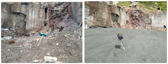
Figure 4.
Sampling points 10 (left) and 23 (right).
The averages of Hg gas measured while workers were on site might be used to evaluate working conditions.
2.2. EN-689:2018 Standard Application
EN-689:2018 provided guidelines for an accurate sampling process [43]. A group of employees exposed to a chemical agent at a similar level while carrying out their duties is known as an SEG (similar exposure group). The goal of the standard is to ascertain whether work in a similar exposure group SEG is consistent with the OELV created for jobs requiring chemical agent exposure.
In this instance, the SEG is the workers who conduct their work in the area with metallurgical plant demolition debris. The degree of exposure is determined by the average concentration of Hg in the atmosphere over eight hours. The chemical agent is gaseous Hg, with an established OELV of 20,000 ng/m3.
The standard specifies that measurements of exposure to the chemical agent must be conducted to ascertain whether the work is compatible with or adheres to that OELV. The standard allows carrying out only three exposure measurements when exposure is less than 10%, four measurements when exposure is less than 15% or five when exposure is less than 20% of the OELV. However, it is necessary that a minimum of 6 measurements and a statistical analysis must be undertaken when the exposure is anticipated to be greater than 20% of the OELV; this case must be applied to the analysis in this situation. According to the guideline, a measurement must monitor the exposure for a minimum of 2 h to accurately represent an entire 8 h day. The weighted average concentration of Hg gas Ck acquired from the Hg gas measurements at a specific site for two hours is considered one sample, assuming there are n samples.
For each sample, the probability pk that the concentration is less than that of the sample Ck is calculated:
On a log-probability paper, the observed exposure Ck values are organised in ascending order and plotted on the horizontal axis against the corresponding probabilities pk on the vertical axis. These findings are distributed lognormally, as evidenced by the solid fit for the straight line [43].
These data must be transformed into the geometric mean GM and geometric standard deviation GSD using the following formula:
This test compares the 95th percentile distribution of the results with the 70% upper confidence limit (UCL). Geometric mean (GM) and standard deviation (GSD) determine UCL. Then, the variable UR is calculated:
The UT variable, tabulated under n (Table 1), must be used to verify the UR value.

Table 1.
UT variable tabulation according to UNE-EN-689:2018 standard.
If UR ≥ UT, then the conclusion is compliant with the OELV.
If UR < UT, then the conclusion is non-compliant with OELV.
Statistical analysis results can be used to decide the interval from the initial compliance test before periodic measurements. Assuming that the results indicate that the SEG complies with a fraction j of the OELV, the procedure is as follows. First, we need to calculate the value of j and then the interval T (months):
- If j < 0.25, then T = 36 months.
- If 0.25 < j < 0.5, then T = 30 months.
- If j > 0.5, then T = 24 months.
Nevertheless, as demonstrated later, this procedure cannot be applied in the case study.
2.3. Biological Markers
Mercury is present in the body in three different forms. The first is as a pure element, without combining (“elemental mercury”), the second is by forming salts or inorganic compounds such as chlorides, sulfides, sulfates, and nitrates (“inorganic mercury”), and the third is by combination with Carbon to form organic compounds such as methylmercury (“organic mercury”). A study performed in Asturias in 2013 [44] showed that the relationship between inorganic Hg and total Hg in the blood is, on average, 50–55%.
Biological marker and regulated biological marker levels are fundamental tools in the control of worker health. In Spain, the legally accepted biological markers are the concentration of total inorganic Hg in blood CHg-B (μg/L) and the concentration of total inorganic Hg in urine related to creatinine CHg-U (μg/g). The limit values established by the National Institute for working safety and health (Instituto Nacional de Seguridad y Salud en el Trabajo, INSST) are recorded in Table 2.
Table 2.
Biological mercury levels according to INSST [45].
Drake et al. [46] state, using data from workers exposed to mercury in gold mining operations, that creatinine is present in a concentration between 0.5 and 3 g per litre of urine. On the other hand, standard medical information shows that a typical value for creatinine production per day is between 14 and 26 mg/day of creatinine per kg of body mass. Taking the average of 20 mg/day × kg and assuming a 75 kg worker drinks 1.5 L of water daily, we obtain 20 × 75/1.5 = 1000 mg/L = 1 g/L, that is, 1 g of creatinine per litre of urine. Therefore, regarding average workers, the expression CHg-U (µg/gCre) ≈ CHg-U (µg/L) can be used, and the limit for Hg in the urine of 30 µg/gCre is equivalent to the limit of 30 µg/L.
Due to data protection issues, this work does not include any actual results related to biological markers. However, estimating the value of biological markers is very useful in the planning phase, and this is included in the work protocol. The extensive experience obtained in the Almadén mines, Spain, over hundreds of years of mercury exploitation is used for this.
Regarding the relationship between the concentration of Hg in urine and Hg in the work environment, Español Cano [47], citing the WHO, said that there is a proportionality between the inorganic Hg concentration in urine CHg-U (µg/L) and the Hg concentration in the air CHg-A (µg/m3).
where the proportionality factor k takes the value 0.7, which is in accordance with the results of other researchers, although the value of k is slightly different. For example, Yoshida [31] provided data from which it can be deduced that the concentration of inorganic Hg in urine CHg-U is a function of individual exposure, weighted in time CHg-A with the coefficient k = 0.13. In the same way, from the data of Iden et al. [48], in a study among workers of a fluorescent lamp factory, the proportional factor is 0.11. Then, we can assume an average value of k = 0.10 and, using the units ng/m3 for the concentration in the air, for inorganic mercury, we obtain:
Drake et al. [46] proposed a linear relationship between neper logarithms ln(CHg-U) and ln(CHg-A), useful even for very high Hg concentration in the environment. In the range from 5000 to 60,000 ng/m3, both Equations (8) and (9) provide similar results, and both can be used as an approach.
On the other hand, some authors have found a relationship between Hg in urine and Hg in blood. The works of Almadén, Español Cano [47] and Tejero Manzanares [49] established the relationship between the concentrations of inorganic Hg in urine CHg-U and in blood CHg-B (both in µg/L):
from which follows
According to Español Cano [47] citing the WHO, there were no specific symptoms below 35 µg/L mercury in the blood (when ambient concentration is about 0.050 mg/m3 or 50,000 ng/m3). As seen, the legal limit for Hg blood concentration is 10 µg/L.
In a study by Yoshida [31] with a sample of workers in a mercury thermometer factory, the relationship between the concentrations of inorganic Hg in urine CHg-U and blood CHg-B (both in nmol/L) was
When the exposure is below 100 µg/m3, it fits with Almadén ambient mercury concentration values of less than 100 µg/m3, which implies blood concentration values below 400 nmol/L or 80 µg/L (80 micrograms of inorganic Hg per litre of blood). In this case, the following formula can be used:
A very relevant topic is the frequency of biomonitoring controls. Some references can be found in the literature related to mining. A typical one is related to very hard working conditions in mercury mining. For example, Kobal and Dizdarevic [50] described that the miners’ biomonitoring in 1997 was performed every month. There are also some references related to gold mining operations, such those of as Drake et al. [46] or Ramírez [51]; in both cases, the recommendation is to control the biomarkers every six months.
Related to the chlor-alkali industry, Lovejoy and Bell [52], in the year 1973, recommended urine analysis every four months, assuming Hg concentration in urine between 100 and 250 µg/L, increasing the frequency if the concentration increases. More recently, in 2010, Euro Chlor [53] recommended a frequency of sampling urinary mercury concentration of 2 controls/year (every six months) when it is under 20 μg/g creatinine and higher than 4 controls/year (every three months) when it is higher than this value.
Manson [54] analysed different industries in the UK. They recommended a urinary sampling interval for urinary Hg between 1 and 3 months, consistent with the reported toxicokinetics of Hg excretion, according to the medical guidance from the Health and Safety Executive on Hg Exposure MS 12 (1996) [54].
Another practical empirical law is the decrease along the time of the urinary Hg concentration after cessation of exposure. After mercury exposure, Hg in the body decreases. Starting from the initial concentration of Hg in urine CHg-U(0), that is, the one it has when exposure ceases, the concentration CHg-U(t) can be estimated after a time t (days) using the following Ellingesen [55] expression:
The analysis of several independent individuals provides a mean value β = 0.0046. This formula allows determining the concentration in urine that will be present when workers exposed to mercury return to work after a break of t days CHg-U(t), if, at the time the holiday began, the concentration was CHg-U(0). On the other hand, taking a limit for CHg-U =30 µg/L also allows for estimating the total rehabilitation time, that is, the time necessary to eliminate Hg from the body.
Finally, it is interesting to comment on Hg concentration in hair. As many authors have already verified [47], the determination of mercury concentration in hair is not suitable for controlling occupational exposure due to external contamination and because mercury can stably bind to the -SH groups of keratin. In addition, hair analysis provides the value of mercury accumulated over several weeks or even months, not from day to day. However, carrying out Hg measurements in hair can be very useful since they can be conducted with the same environmental control equipment, faster than urine or blood analysis.
The concentration of Hg in hair is not a biological marker accepted by the authorities; nevertheless, it is interesting to observe relationships between Hg in hair and blood or urine. Español Cano [47] points out that a linear correlation has been established between the levels of mercury in hair CHg-H and the total mercury in blood CHg-B, with relationships varying from 300 to 500. According to Diez et al. [56], citing Phelps et al. [23] and the World Health Organisation (WHO), the Hg ratio in hair to total Hg in the blood is 250 to 1. Assuming a blood density of 1.06 kg/L, there are
where CHg-B is in µg/L, and CHg-H is in mg/kg (or what is the same ppm).
After Packull-McCormick et al. [57], using the 250:1 ratio derived by the World Health Organisation to estimate blood mercury concentrations from hair mercury concentrations substantially overestimates blood mercury concentrations. However, geometric mean site-specific hair-to-blood mercury ratios can estimate central tendency measures for blood mercury concentrations from hair mercury concentrations at a population level.
Diez et al. [56] cited Harada et al. [58] to establish a limit of 10 ppm for the concentration of Hg in hair in workers exposed to Hg. The WHO sets no specific symptoms below 35 µg/L in the blood (ambient concentrations of 0.050 mg/m3 or 50,000 ng/m3). As can be seen, there is consistency with the limits since 10 ppm in hair corresponds to approximately 40 µg/L, which is of the same order.
3. Results and Discussion
3.1. Results in Areas with Demolition Debris from the Metallurgical Plant Building
There are two areas where demolition debris accumulates:
- Point 10: area with demolition debris in its original location;
- Point 23: area with demolition rubble covered with slag and ash (next to the previous one).
In previous studies, the following conclusion was reached: the demolition rubble from the metallurgical plant, point 10, behaved as an emitting source. At this point, the emissions of Hg gas and its concentration in the air strongly depended on the temperature. With temperatures around 30 °C, the average Hg gas concentration in the rubble air reached almost 60,000 ng/m3. Figure 5 shows the rubble area and a Hg gas record obtained at 15.5 °C; the average concentration reached 13,680 ng/m3.
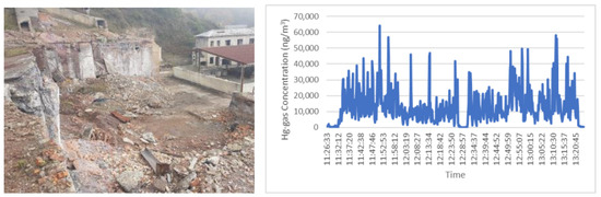
Figure 5.
The area at point 10 and a record of Hg gas concentration.
One of the tasks to be carried out in the project is to use industrial waste (blast furnace slag and coal ashes) to improve the environment of the old mining–metallurgical facilities. For this reason, a large part of the demolition rubble was covered with slag and ashes, creating a new work zone named point 23.
A photo of the new area is shown in Figure 6. It is verified that the layer of slag and ash stops the emission of the rubble that is covered. For this reason, the area begins behaving like other surrounding points in which the Hg gas concentration in the air results from the dispersion of Hg gas from the rubble that remains uncovered. Figure 6 shows a record of the monitoring of gaseous Hg at point 23 on the same day. With a temperature of 15.5 °C, the average concentration of Hg in the air is only 814 ng/m3 (less than 10% of the OELV), utterly different from point 10 previously analysed.
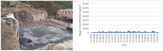
Figure 6.
The area at point 23 and a record of Hg gas concentration.
Table 3 and Figure 7 summarise the analysis for points 10 and 23. In the case of point 10, it is seen that the concentration of gaseous Hg increases with temperature, following the same exponential pattern previously determined by Rodríguez et al. [38]. Since this is the critical point of the site, 24 measurement campaigns were carried out in different temperature conditions, and in all cases, the 20% OELV (4000 ng/m3) was exceeded. Therefore, to determine under which requirements works can be carried out in point 10 following EN-689:2018, a complete statistical analysis must be carried out (see the next section).
Table 3.
Measurements in points 10 and 23.
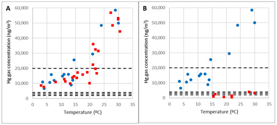
Figure 7.
Gaseous Hg concentration at point 10 (A) and point 23 (B), current (red) and previous measurements (blue).
Figure 7A shows that below 20 °C, the average readings are below the OELV (20,000 ng/m3). Likewise, it is observed that above 25 °C, the temperatures are higher than the OELV. However, there is a range of temperatures between 20 °C and 25 °C in which it can be above or below, and we believe that the explanation for this is related to the weather.
Temperatures around 30 °C are relatively infrequent in Asturias and occur with very stable conditions, with clear skies and no wind. The high solar radiation favours the emission of Hg gas, and the absence of wind prevents its dispersion, thus increasing its concentration in the air. The same happens with the coldest days in Asturias, less than 5 °C, and typical winter days with clear skies that favour frost and little wind. However, in the more normal temperature range of 10 °C to 15 °C, rain, wind, clouds, or clearings may cause Hg gas emission to fluctuate.
Wind influence is evident. With temperatures around 20 °C and more or less stable conditions, concentrations around 20,000 ng/m3 have been found. However, on one day with a temperature of 20 °C but with strong gusts of wind, the concentration drastically dropped to 10,000 ng/m3.
It should be noted that the work with the rubble was always carried out at temperatures below 15 °C, in conditions compatible with the regulations. The measurements obtained with temperatures above 15 °C were recorded in the absence of any other work and only to determine how the temperature influenced the Hg gas concentration. For the measurements carried out with very high concentrations (always less than 60,000 ng/m3), the presence of personnel was reduced to about 2–3 min that it took to place the measurement equipment on top of the rubble (always less than the 15 min allowed by the legislation).
Another critical aspect, typical in underground coal mining, is that no worker carries out a task alone in this area; to work in this area, there must be at least two workers together.
At point 23, it is verified that with temperatures around 20 °C, the concentration of gaseous Hg in the environment is moderate, similar to other site points. Therefore, five measurements were carried out to analyse the exposure to gaseous mercury. All of them were below 15% of the OELV, showing that the work at point 23, on the rubble covered with ash and slag, is compatible with the mercury legislation on air, and it is up to temperatures of the order of 20 °C.
Since work on the rubble was never carried out at temperatures above 15 °C, the standard does not impose more samples to be carried out to analyse the OELV limit. However, two more measurements were conducted to see the effect of slag and ash, reducing and even eliminating gaseous mercury emissions at the highest temperatures in Asturias (around 30 °C).
In conclusion, the concentration of gaseous Hg dropped drastically after covering the rubble with slag and ashes. It should be noted that covering the contaminated material is an effective safety measure for protecting workers.
3.2. Application of the EN-689:2018 Standard and Development of a Risk Prevention Criterion
As previously stated, to determine under what conditions work can be carried out in point 10 following the EN-689:2018 standard, the statistical analysis defined in the same standard must be carried out.
There are 24 samples of Hg gas in the air in the area of demolition debris Ck = C10 (ng/m3) taken in the temperature range 5 °C to 30 °C. A first statistical analysis of all of them already provides precious information. Following the standard, the graph of Figure 8A is represented, which indicates that conditions cannot be considered homogeneous in the temperature range of 5 °C to 30 °C. The calculation of the parameters UR = 0.028 < UT = 1.846 shows no compliance with the OELV.
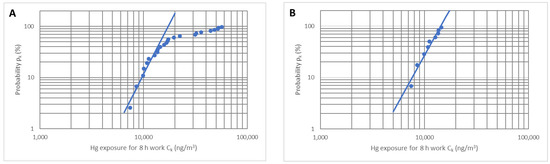
Figure 8.
Analysis of the log-normal distribution for the ranges 5–30 °C (A) and 5–15 °C (B).
It is also noted that the graph indicates that there are different sets of conditions or trends and that temperature may be the critical variable that defines the difference between them. Up to Ck ≈ 14,000 ng/m3, a line representing more or less homogeneous conditions can be fitted. However, the data do not follow that trend from that concentration, which could indicate other situations. The concentration of 14,000 ng/m3 is reached at temperatures around 15 °C. Therefore, homogeneous working conditions could be working at temperatures below 15 °C.
Repeating the analysis with the nine data obtained in approximate conditions with θ < 15 °C and Ck < 14,000 ng/m3, we see that they conform to a log-normal distribution (Figure 8B) with a correlation coefficient r2 = 0.94. The calculation of the parameters UR = 2.562 > UT = 2.035 indicates compliance with the OELV. The work of 8 h/day and 40 h/week follows the OELV = 20,000 ng/m3.
On the other hand, the calculation provides j = 0.89, meaning that the period until a new reassessment should be T = 24 months. However, the dependence of the mercury concentration on the ambient temperature makes the working conditions change quickly, and then this interval must be diminished. Due to this, the calculation of T based on j will not be carried out in the following.
It is clear that when Ck > OELV = 20,000 ng/m3, the conditions for working 8 h/day and 40 h/week are not met. As seen in Figure 7A, this concentration is reached at 20 °C; below that temperature, the concentration is always lower than the OELV.
It is necessary to analyse the conditions with temperatures between 15 °C and 20 °C to check for limitations. Using the six available data obtained between 15.5 °C and 21.1 °C, it is concluded that in this temperature range, there is no compliance with the OELV. Therefore, working 8 h/day and 40 h/week is unacceptable regarding occupational mercury limits. In addition, there is also no conformity if the six available data are used with temperatures between 14.5 °C and 20 °C. This is because, as we choose a range closer to 20 °C, the concentration becomes closer to the OELV, and non-conformance is more likely than at lower temperatures. The solution to this problem is to limit the number of working hours per day so that the equivalent dose is less than the OELV.
Let us assume that 6 h are worked every day at point 10, 1 h at point 3 (we assume a concentration of C3 = 1000 ng/m3) and 1 h at point 7 (C7 = 4000 ng/m3). If Ck1…Ck6 are the six values used for the analysis, assuming that 8 h are worked, the new representative values to carry out the analysis are
If the six values are taken between 14.5 °C and 20 °C, it can be found that there is compliance with the OELV (UR = 2.940 > UT = 2.187). However, if the six representative points are taken between 15.5 °C and 21.1 °C, working 6 h per day is not possible, even if the remaining two hours are rested at point 3. In this case, the values to be used are
The analysis result is UR = 1.978 < UT = 2.187; that is, there is no compliance with the OELV.
Only if we reduce the number of working hours in point 10 to 5 is compliance fulfilled, even assuming that the remaining three hours are worked in point 7 (C7 = 4000 ng/m3):
Figure 9A represents the log-normal distribution for this case. The calculation provides UR = 2.502 > UT = 2.187, which means compliance with the OELV = 20,000 ng/m3.
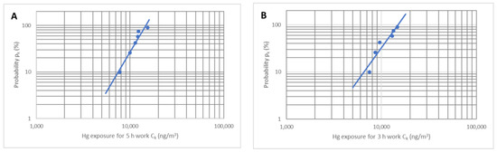
Figure 9.
Analysis of the log-normal distribution for the ranges 15 °C to 20 °C (A) and 20 °C to 25 °C (B).
Therefore, the best solution to be able to carry out work at point 10 when the temperature is between 15 °C and 20 °C is to limit the work at that point to only 5 h/day, with a possiobility to carry out work at any other point in the remaining three hours.
The analysis can now be repeated in the interval of 20 °C to 25 °C. In that interval, the concentration fluctuations can be huge; thus, the six available data vary between 16,600 and 35,883 ng/m3.
Repeating the previous analysis, it is found that, with temperatures between 20 °C and 25 °C, at point 10, work can be carried out for up to a maximum of 3 h, provided that the remaining 5 h were worked at points with a concentration of less than 2000 ng/m3 (points 4 or 21). The values to be used are calculated as follows:
The log-normal distribution is depicted in Figure 9B. Considering that UR = 2.245 > UT = 2.187, it is concluded that there is compliance with the OELV = 20,000 ng/m3.
Based on the results of the previous analysis, it is possible to define a Risk Prevention Criterion that appears in Table 4. Three work scenarios are defined with which the classic green–orange–red colours are associated.
Table 4.
Risk prevention criterion for exposure to Hg according to the EN-689:2018 standard.
The green stage occurs when the Hg concentration is below 10,000 ng/m3 (typically with the temperature below 10 °C). In this case, working in the demolition rubble area for 8 h/day (standard shift) is possible. However, it must be said that gas semi-masks are always used at work, and the authority recommends a 0.5 h break after continuous work for 1 h (although due to operational reasons, in our case, a 1 h break is adopted after 2 h of continuous working). Therefore, even if the conditions are favourable, the maximum number of working hours per day is 6 h/day.
The orange scenario is defined in the Hg concentration range of 10,000 to 20,000 ng/m3 (temperature range of 10 °C to 20 °C). If it can be ensured that the Hg in the air is below 15,000 ng/m3, the considerations of the green procedure are valid. However, if the Hg concentration exceeds 15,000 ng/m3 (typically above 15 °C), the maximum working hours are 5 h daily. Considering it is possible to work 6 h/day in the most favourable conditions, the orange scenario does not represent a drastic change in routine work.
Above 20,000 ng/m3 (typically above 20 °C), we enter the red stage. Some work in rubble areas is allowed only in the range of 20,000 to 40,000 ng/m3 (20 °C to 25 °C), but with some extreme restrictions since it is not possible to work more than 3 h/day. From above 40,000 ng/m3 (typically above 25 °C), work with demolition rubble is prohibited without taking additional measures. Only particular jobs (such as sampling) could be carried out with a maximum of 1 h/day, distributed into four periods of 15 min/hour for 4 h.
Work with temperatures between 20 °C and 25 °C, with concentrations that could reach 40,000 ng/m3, represents the worst conditions in which practical work can be carried out following the legislation. The limitation to 3 h/day of work, or 60 h/month, is the same order as the 48 h/month of normal conditions in Spanish mercury mining, with average concentrations of 121,000 ng/m3 [47]. It is seen that this criterion follows the experience in the mercury mines, although, by the requirement of the legislation, it is even more conservative.
This risk prevention criterion has the advantage of being simple and mnemonic: the mercury concentrations in the environment at typical working temperatures, 10 °C, 15 °C and 20 °C, are 10,000, 15,000 and 20,000 ng/m3, respectively.
Finally, from all of the above, it is deduced that a fundamental variable, temperature, deterministically controls gaseous Hg emissions. For this reason, setting a temperature range is equivalent to defining homogeneous working conditions. The fluctuations in the concentration of Hg gas within that temperature range would be determined by other variables related to the climate, such as wind, solar radiation or rain.
It must be kept in mind that the work has to be planned and carried out according to the Hg gaseous concentration. The temperature variable allows the quick estimate of the Hg concentration and decision on the work during the planning and execution phases. Nevertheless, if continuous monitoring enables us to determine that the Hg concentration is less than 10,000 ng/m3, the work could be carried out according to the green scenario, although the temperature is higher than 10 °C. It can occur, for example, if the strong wind makes the concentration under the expected Hg concentration for this temperature.
Respecting the frequency of the monitoring of Hg in the air, we must remember that at our latitude, the temperature can be over 15 °C in any period of the year, even during the winter. Consequently, the works for the next days must be planned based on the Spanish Meteorological Agency’s (AEMET) forecast. Simultaneously, it is recommended to carry out control monitoring every month, according to Spanish Mercury Technological Center [59]. It is also recommended to diminish the interval to 2 weeks with medium and high temperatures.
When the temperature is over 15 °C, additional measures can be recommended, especially if we want to increase the working time to 6 h. Some are not expensive or difficult to implement, such as covering the contaminated rubble (in our case, with ash and slag), using a long-arm excavator that allows the driver to be far from the rubble, and using a full mask with HgP3 filters instead of a semi mask with HgP3 filters, etc. In the case of taking measures that diminish the concentrations of Hg in the working place, the working time could be increased.
The Spanish law does not define the frequency of the workers’ biomonitoring, and the law only requires that all workers must be checked at least once a year. For specific risks, the number of biomonitoring controls must be defined by the company’s occupational health service physician after assessing the workplace risks. The Mercury Technological Center has established for its employees who work in exposed places to carry out urine analysis every month and blood analysis every 3 months, which can be taken as a first reference.
3.3. Analysis of the Actual Work with the Demolition Rubble of the Metallurgical Plant
As can be deduced from the previous analyses, from the point of view of worker health and safety, the work with demolition rubble is the most critical. It requires careful planning and strict onsite control measures. Typically, only three operators work, and in some cases four (Table 5). External personnel only participate in placing the HDPE waterproof sheet (another four people), although they only work one day. Several illustrative photographs of these tasks are shown in Figure 10, Figure 11 and Figure 12.
Table 5.
Tasks carried out in the rubble area (point 10 and surroundings).
Figure 10 (left) shows the development of task 1, where the rubble is removed with a backhoe excavator to carry out task 2, building a concrete slab, Figure 10 (right). The photograph of Figure 10 (right) shows the personal protective equipment used by the workers. In addition to the standard personal protective equipment PPE (hard hat, safety boots), the specific protection necessary to work in the area can be seen: integral protection cover, gloves protecting against chemical risks, safety glasses and a half mask filtering gases and mercury vapours HgP3.

Figure 10.
(Left): task 1 (debris removal); (Right): task 2 (concrete slab construction).
Figure 10.
(Left): task 1 (debris removal); (Right): task 2 (concrete slab construction).

Figure 11 (left) shows the perimeter wall construction, and Figure 11 (right) shows the placement of the HDPE sheet. It is the task that requires the most personnel. Firstly, the Hg gaseous concentration meter in the environment is part of the real-time monitoring frequently carried out as a control measure on site.

Figure 11.
(Left): task 3 (perimeter wall construction); (Right): task 4 (HDPE sheet placement).
Figure 11.
(Left): task 3 (perimeter wall construction); (Right): task 4 (HDPE sheet placement).

Figure 12 (left) illustrates task 6 of filling with demolition rubble, and the same Figure 12 (right) shows the work of tasks 5, 7 and 8 of filling with by-products (slag and ashes transported in tip trucks).

Figure 12.
(Left): task 6 (excavator in rubble), (Right): tasks 7, 8 (dump truck).
Figure 12.
(Left): task 6 (excavator in rubble), (Right): tasks 7, 8 (dump truck).

As seen below, the knowledge provided by the previous studies makes it possible to carry out the planning and control of the work systematically and relatively simply. The procedure for planning the work with the rubble (point 10) is as follows:
- The dates on which the work will be carried out are defined.
- The temperature θ (°C) is defined with the average monthly value of the last 10 years according to the Spanish Agency for Meteorology (Agencia Española de Meteorología, AEMET).
- The allowed work period nmax = 6 h/day is established as a first approximation.
- The concentration at point 10 and the concentration at other alternative points are estimated (for simplicity, it is assumed that they are at least 50 m from point 10):
- The weighted average exposure to gaseous Hg in an 8 h workday is estimated as
- The average concentration of inorganic Hg in urine and blood is estimated:
- It is checked if the Ceq weighted average exposure is in accordance with the OELV = 20,000 ng/m3.
- The concentrations in urine CHg-U and blood CHg-B are compared with the OELV 30 µg/L and 10 µg/L.
Table 6 summarises the calculations. In all cases, the control variables are below the OELV limits imposed by the legislation; the work planned this way would follow the legislation.
Table 6.
Analysis of the work to be carried out in the planning phase.
On the other hand, using the same procedure described, a work control can be carried out simultaneously with the development of the works or retrospective analysis of the work once completed, verifying that the safety and health parameters are met.
In the actual case of the SUBproducts4LIFE project, the work was carried out in two phases. The first half of the initial area was worked on, and then the other half, so the tasks were repeated, and their number increased. Part of the monitoring and control of Hg gas was carried out while the work was carried out, although it is now presented as a retrospective analysis. In this case, the data used are the real data, and the risk prevention criteria were used as a guide since they were defined with the legal OELV values of the INSST measuring the mercury in the air according to the EN-689:2018 standard. This demonstrates that the work is compatible with that OELV.
The process was the following:
- The best months to work were chosen: those in which the average temperature is below 15 °C according to the prevention criteria (in Asturias, all except those in summer, June, July, August and September).
- The daily temperature was recorded, or the average daily temperature in the area provided by the meteorological services (AEMET) was used. The graph of Figure 13A shows the daily variation of the real temperature, as well as the average temperature of the period.
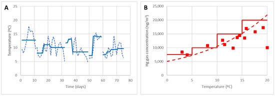 Figure 13. (A): Daily temperature (dotted line) and the average for each period (continuous line). (B): Estimation of the concentration with the empirical model (dotted line) and with the risk prevention criterion (continuous line).
 - The allowed work time was established according to the prevention criteria: nmax = 6 h/day as the temperature is always θ < 15 °C.
- The concentration in point 10 was estimated based on the prevention criteria. In Figure 13B, it is seen that also the curve of the empirical model (dotted) could be used to define the concentration at point 10 at a given temperature; however, as said, it is easier to use the concentration specified by the risk prevention criteria (solid line) according to EN-689:2018.
- The equivalent exposure Ceq was calculated assuming that, with the regulatory breaks, 6 h/day was spent at point 10, 1 h/day at point 3 and 1 h/day at point 7 (the most unfavourable work point). Assuming C3 ≤ 1000 ng/m3 and C7 ≤ 4000 ng/m3, the weighted average exposure to gaseous Hg in an 8 h shift was estimated.
It was checked whether the Ceq weighted average exposure was in accordance with the OELV = 20,000 ng/m3.
Table 7 shows the results. In addition to the indicated data, those significant periods without work concerning the body’s capacity to eliminate Hg were also noted. The general result is that the average exposure of a worker is approximately 50% of the OELV maximum permitted dose, so it must be concluded that the work was carried out in conditions in compliance with the legal limits.
Table 7.
Retrospective analysis of the work performed.
It must be said that the calculation carried out is conservative, since it is considered that all the tasks carried out involve the handling of the rubble, which is not true. The tasks related to the construction of the walls, the concreting of the floor, etc., were carried out at the limits of the rubble zone, where the concentration drops to half. On the other hand, it is assumed that working with rubble implies being on the rubble 100% of the time, something that is not true; some of the work can be conducted near the debris boundary where concentrations are already half those in the centre. In addition, it is assumed that no measure is carried out to diminish the Hg gaseous emission, which is also conservative. If necessary, covering the rubble with subproducts diminishes the Hg concentration, significantly improving the working conditions.
As can be deduced from Table 6, the work should be carried out during different months over 1.5 years. Nevertheless, due to a significant delay in obtaining permits from authorities and mainly due to the COVID-19 pandemic, the work was carried out for 2.5 years, as shown in Table 7. This means that there were short periods of continuous working (maximum 16 days) and long periods without working, which is very positive from a health and safety point of view.
Regarding controlling worker health based on biological markers, the results are not available for the actual case. Therefore, they were not included in the retrospective analysis. As the number of workers involved is minimal, the anonymity required by the data protection law cannot be guaranteed, which is why it was left out of the scope of this study.
The work in mining tailings contaminated by metals, specifically by Hg, is very topical because administrations must restore decommissioning mining facilities and industrial buildings highly contaminated with mercury. In addition, nowadays, tailings are an emerging market opportunity.
In this context, all research aimed at the health and safety of workers is very important, so having a replicable methodology is very useful.
On the other hand, the information is sensitive, and companies are not inclined to publish the results. The results of our work, with valuable field data and a new perspective, could benefit other engineers and/or technicians in charge of Health and Safety working in highly contaminated areas.
The work conducted above was to illustrate or provide an example of how the methodology is used at two different and very interesting moments in any project:
- (a)
- During planning (prediction);
- (b)
- After executing the jobs (back-analysis).
To be sure that predictions can be offered and used during planning, it is important to demonstrate the causal relationship between the variables evolved.
The fact that the actual final results are similar to those predicted is a consequence of several underlying causal phenomena: the physical law that determines the temperature as a function of the time of year, the physical law that defines the Hg emission as a function of the temperature and the rules that determine the concentration of Hg in blood and urine in a person who breathes air in which there is gaseous Hg. Based on underlying physical laws, causality is assured.
It is important to note that with the data of the last 10 years, the average value of the average, minimum and maximum daily temperatures are θmedM = 13.2 °C, θminM = 8.18 °C and θmaxM = 18.33 °C, and the average temperature is reached at the end of the month of April (month 4, t = 120 days) and that the temperature varies with a sinusoidal law in which the period is the 365 days of the year T = 365 days:
This law, together with the law that governs the emission of gaseous Hg and its concentration on the source, Equation (1), and those that govern the concentration of Hg in urine and blood, Equations (10) and (11), ensure that, ultimately, conducting work at one time or another of the year is the cause of the varying Hg levels in a worker’s body.
3.4. Brief Analysis under ESG Criteria
The sustainable development of the global economy and society calls for the practice of the environmental, social and governance (ESG) principle. The ESG principle has been developing for almost 20 years following its formal proposal in 2004. Over the past decades, ESG factors have become increasingly relevant for investors and stakeholders (creditors, regulators, etc.). In this way, it is helpful to contextualise our findings in light of this growing trend (increasing relevance of ESG), especially considering that the results speak to the “E” (environmental) and the “S” (social, as far as worker safety is a societal problem) of ESG criteria. As Dantas (2021) [60] pointed out, institutional investors increasingly use ESG factors in their portfolio when making decisions.
Taking different proposals for the ESG criteria as a reference, what is described in this work can positively assess various topics related to pillar (E) and pillar (S), as presented in Table 8.
Table 8.
Topics in which the research would be positively assessed according to different ESG criteria proposals.
4. Conclusions
Managing demolition waste from a mercury mine facility can be a significant hazard regarding Hg emissions, so it is crucial to plan the work carefully. The research developed a proper sampling procedure following the standard EN-689:2018 to ensure the workers’ protection; the sampling campaigns included at least 2 h of sampled periods in different conditions, and all the tasks carried out in the restoration project were evaluated.
A working protocol with three scenarios (green, orange, red) was developed to calculate the maximum working hours in the function of the forecast temperature, a valuable tool for planning the works. In the same way, it was checked that the empirical model developed in la Soterraña by Rodríguez [38] fits in the measurements allowing forecasting of the workers’ exposure all over the year. Evaluating the Hg gas concentration in the air, it is possible to estimate the biological markers such as Hg in blood or Hg in urine, essential parameters to protect the workers’ health.
Lastly, it was demonstrated that covering high-emission Hg rubble with furnace slag and ashes reduces Hg gas emissions is a vital engineering control tool to avoid or minimise Hg gas exposition to workers and an important environmental measure to minimise the mercury emissions in la Soterraña.
All the aspects defined in this study (mercury gaseous monitoring system, risk prevention criterion or working protocol) were helpful to the performance of the work under safety conditions in this specific place: the rubble from the demolition of the metallurgical plant. These aspects should only be used as a guide for other different sites. Nevertheless, the defined methodology that measures the Hg gas concentration, relates it with other variables such as the temperature, develops a risk prevention criterion and defines a working protocol can be extrapolated to any other site, but it is an empirical investigation, and therefore it would only be applicable in similar conditions unless the model is readjusted.
Researching the emissions of different gases in abandoned tailings or debris and determining emission laws can be a line of research for the future, both from an environmental point of view, especially if the temperatures will rise, and from a health and safety point of view, if mining dumps become of beneficial interest.
The main practical implication is to use this research as a working guide for work on tailings contaminated with metals, which is becoming increasingly frequent.
Author Contributions
Conceptualisation, R.R. and H.G.-G.; methodology, R.R. and H.G.-G.; validation, R.R., H.G.-G., Á.P. and Z.H.; investigation, R.R., H.G.-G. and Z.H.; data curation, R.R. and H.G.-G.; writing—original draft preparation, R.R., H.G.-G. and Z.H.; writing—review and editing, H.G.-G.; supervision, R.R.; project administration, R.R., Á.P. and Z.H.; funding acquisition, R.R. and Á.P. All authors have read and agreed to the published version of the manuscript.
Funding
The authors would like to thank the program LIFE of the European Commission for the funding received for the project SUBproducts4LIFE (reference LIFE16 ENV/ES/000481).
Institutional Review Board Statement
Not applicable.
Informed Consent Statement
Not applicable.
Data Availability Statement
The data presented in this study are available within the manuscript.
Acknowledgments
Authors would like to thank the collaboration of the institutions and private companies that participated in the project SUBproducts4LIFE: Biosfera consultoría Medioambiental (BIOSFERA), Escorias y Derivados (EDERSA), Global Service (GService), Hidroeléctrica del Cantábrico (EDP), Instituto Asturiano de Prevención de Riesgos Laborales (IAPRL), Recuperación y Renovación (R&R) and Universidad de Oviedo (UNIOVI). Finally, the collaboration of sponsors Arcelor Mittal, Ingeniería de Montajes Norte SA (IMSA), Asturbelga de Minas, Lena Council, and the Instituto Nacional de Silicosis (INS) is also greatly appreciated.
Conflicts of Interest
The authors declare no conflict of interest.
References
- Hylander, L.D.; Meili, M. 500 Years of Mercury Production: Global Annual Inventory by Region until 2000 and Associated Emissions. Sci. Total Environ. 2003, 304, 13–27. [Google Scholar] [CrossRef]
- UN Environment Programme. Guideline for Decommissioning of Mercury Chlor-Alkali Plants. Available online: http://www.unep.org/resources/report/guideline-decommissioning-mercury-chlor-alkali-plants (accessed on 18 April 2023).
- Finster, M.E.; Raymond, M.R.; Scofield, M.A.; Smith, K.P. Mercury-Impacted Scrap Metal: Source and Nature of the Mercury. J. Environ. Manag. 2015, 161, 303–308. [Google Scholar] [CrossRef]
- Randall, P.; Chattopadhyay, S. Advances in Encapsulation Technologies for the Management of Mercury-Contaminated Hazardous Wastes. J. Hazard. Mater. 2004, 114, 211–223. [Google Scholar] [CrossRef]
- Wang, S.; Feng, X.; Qiu, G.; Shang, L.; Li, P.; Wei, Z. Mercury Concentrations and Air/Soil Fluxes in Wuchuan Mercury Mining District, Guizhou Province, China. Atmos. Environ. 2007, 41, 5984–5993. [Google Scholar] [CrossRef]
- Gustin, S.M.; Coolbaugh, M.; Engle, M.; Fitzgerald, B.; Keislar, R.; Lindberg, S.; Nacht, D.; Quashnick, J.; Rytuba, J.; Sladek, C.; et al. Atmospheric Mercury Emissions from Mine Wastes and Surrounding Geologically Enriched Terrains. Environ. Geol. 2003, 43, 339–351. [Google Scholar] [CrossRef]
- Feng, X. Mercury Pollution in China—An Overview. In Dynamics of Mercury Pollution on Regional and Global Scales: Atmospheric Processes and Human Exposures around the World; Springer: Boston, MA, USA, 2005; pp. 657–678. ISBN 978-0-387-24493-8. [Google Scholar]
- Loredo, J.; Ordóñez, A.; Gallego, J.R.; Baldo, C.; García-Iglesias, J. Geochemical Characterisation of Mercury Mining Spoil Heaps in the Area of Mieres (Asturias, Northern Spain). J. Geochem. Explor. 1999, 67, 377–390. [Google Scholar] [CrossRef]
- Lin, Y.; Larssen, T.; Vogt, R.D.; Feng, X. Identification of Fractions of Mercury in Water, Soil and Sediment from a Typical Hg Mining Area in Wanshan, Guizhou Province, China. Appl. Geochem. 2010, 25, 60–68. [Google Scholar] [CrossRef]
- Ordóñez, A.; Álvarez, R.; Charlesworth, S.; Miguel, E.D.; Loredo, J. Risk Assessment of Soils Contaminated by Mercury Mining, Northern Spain. J. Environ. Monit. 2011, 13, 128–136. [Google Scholar] [CrossRef]
- Scholtz, M.T.; Van Heyst, B.J.; Schroeder, W.H. Modelling of Mercury Emissions from Background Soils. Sci. Total Environ. 2003, 304, 185–207. [Google Scholar] [CrossRef]
- Kotnik, J.; Horvat, M.; Dizdarevič, T. Current and Past Mercury Distribution in Air over the Idrija Hg Mine Region, Slovenia. Atmos. Environ. 2005, 39, 7570–7579. [Google Scholar] [CrossRef]
- Loredo, J.; Soto, J.; Alvarez, R.; Ordóñez, A. Atmospheric Monitoring at Abandoned Mercury Mine Sites in Asturias (NW Spain). Environ. Monit. Assess. 2007, 130, 201–214. [Google Scholar] [CrossRef]
- Zhu, J.; Wang, D.; Liu, X.; Zhang, Y. Mercury Fluxes from Air/Surface Interfaces in Paddy Field and Dry Land. Appl. Geochem. 2011, 26, 249–255. [Google Scholar] [CrossRef]
- Qiu, G.; Feng, X.; Meng, B.; Sommar, J.; Gu, C. Environmental Geochemistry of an Active Hg Mine in Xunyang, Shaanxi Province, China. Appl. Geochem. 2012, 27, 2280–2288. [Google Scholar] [CrossRef]
- Cabassi, J.; Tassi, F.; Venturi, S.; Calabrese, S.; Capecchiacci, F.; D’Alessandro, W.; Vaselli, O. A New Approach for the Measurement of Gaseous Elemental Mercury (GEM) and H2S in Air from Anthropogenic and Natural Sources: Examples from Mt. Amiata (Siena, Central Italy) and Solfatara Crater (Campi Flegrei, Southern Italy). J. Geochem. Explor. 2017, 175, 48–58. [Google Scholar] [CrossRef]
- Lindberg, S.E.; Kim, K.H.; Meyers, T.P.; Owens, J.G. Micrometeorological Gradient Approach for Quantifying Air/Surface Exchange of Mercury Vapor: Tests over Contaminated Soils. Environ. Sci. Technol. 1995, 29, 126–135. [Google Scholar] [CrossRef]
- Llanos, W.; Kocman, D.; Higueras, P.; Horvat, M. Mercury Emission and Dispersion Models from Soils Contaminated by Cinnabar Mining and Metallurgy. J. Environ. Monit. 2011, 13, 3460–3468. [Google Scholar] [CrossRef]
- Matanzas, N.; Sierra, M.J.; Afif, E.; Díaz, T.E.; Gallego, J.R.; Millán, R. Geochemical Study of a Mining-Metallurgy Site Polluted with As and Hg and the Transfer of These Contaminants to Equisetum Sp. J. Geochem. Explor. 2017, 182, 1–9. [Google Scholar] [CrossRef]
- McNutt, M. Mercury and Health. Science 2013, 341, 1430. [Google Scholar] [CrossRef]
- Kim, K.-H.; Kabir, E.; Jahan, S.A. A Review on the Distribution of Hg in the Environment and Its Human Health Impacts. J. Hazard. Mater. 2016, 306, 376–385. [Google Scholar] [CrossRef]
- Wu, Z.; Zhang, L.; Xia, T.; Jia, X.; Wang, S. Heavy Metal Pollution and Human Health Risk Assessment at Mercury Smelting Sites in Wanshan District of Guizhou Province, China. RSC Adv. 2020, 10, 23066–23079. [Google Scholar] [CrossRef]
- Phelps, R.W.; Clarkson, T.W.; Kershaw, T.G.; Wheatley, B. Interrelationships of Blood and Hair Mercury Concentrations in a North American Population Exposed to Methylmercury. Arch. Environ. Health Int. J. 1980, 35, 161–168. [Google Scholar] [CrossRef]
- Koenigsmark, F.; Weinhouse, C.; Berky, A.J.; Morales, A.M.; Ortiz, E.J.; Pierce, E.M.; Pan, W.K.; Hsu-Kim, H. Efficacy of Hair Total Mercury Content as a Biomarker of Methylmercury Exposure to Communities in the Area of Artisanal and Small-Scale Gold Mining in Madre de Dios, Peru. Int. J. Environ. Res. Public Health 2021, 18, 13350. [Google Scholar] [CrossRef]
- Garcia Gonzalez, H.; García-Ordiales, E.; Diez, R.R. Analysis of the Airborne Mercury and Particulate Arsenic Levels Close to an Abandoned Waste Dump and Buildings of a Mercury Mine and the Potential Risk of Atmospheric Pollution. SN Appl. Sci. 2022, 4, 76. [Google Scholar] [CrossRef]
- WHO. Mercury and Health. 2017. Available online: https://www.who.int/news-room/fact-sheets/detail/mercury-and-health (accessed on 1 February 2021).
- Saturday, A. Mercury and Its Associated Impacts on Environment and Human Health: A Review. J. Environ. Health Sci. 2018, 4, 37–43. [Google Scholar] [CrossRef]
- Morton, J.; Sams, C.; Leese, E.; Garner, F.; Iqbal, S.; Jones, K. Biological Monitoring: Evidence for Reductions in Occupational Exposure and Risk. Front. Toxicol. 2022, 4, 836567. [Google Scholar] [CrossRef]
- Wcisło, E.; Bronder, J.; Bubak, A.; Rodríguez-Valdés, E.; Gallego, J.L.R. Human Health Risk Assessment in Restoring Safe and Productive Use of Abandoned Contaminated Sites. Environ. Int. 2016, 94, 436–448. [Google Scholar] [CrossRef]
- Lie, A.; Gundersen, N.; Korsgaard, K.J. Mercury in Urine—Sex, Age and Geographic Differences in a Reference Population. Scand. J. Work. Environ. Health 1982, 8, 129–133. [Google Scholar] [CrossRef]
- Yoshida, M. Relation of Mercury Exposure to Elemental Mercury Levels in the Urine and Blood. Scand. J. Work. Environ. Health 1985, 11, 33–37. [Google Scholar] [CrossRef]
- Rumiantseva, O.Y.; Ivanova, E.; Komov, V. High Variability of Mercury Content in the Hair of Russia Northwest Population: The Role of the Environment and Social Factors. Int. Arch. Occup. Environ. Health 2022, 95, 1027–1042. [Google Scholar] [CrossRef]
- Eckley, C.S.; Gilmour, C.C.; Janssen, S.; Luxton, T.P.; Randall, P.M.; Whalin, L.; Austin, C. The Assessment and Remediation of Mercury Contaminated Sites: A Review of Current Approaches. Sci. Total Environ. 2020, 707, 136031. [Google Scholar] [CrossRef]
- González-Valoys, A.C.; Jiménez Salgado, J.U.; Rodríguez, R.; Monteza-Destro, T.; Vargas-Lombardo, M.; García-Noguero, E.M.; Esbrí, J.M.; Jiménez-Ballesta, R.; García-Navarro, F.J.; Higueras, P. An Approach for Evaluating the Bioavailability and Risk Assessment of Potentially Toxic Elements Using Edible and Inedible Plants—The Remance (Panama) Mining Area as a Model. Environ. Geochem. Health 2021, 45, 151–170. [Google Scholar] [CrossRef]
- Wcisło, E.; Bronder, J.; Rodríguez-Valdés, E.; Gallego, J.L.R. Health Risk Assessment of Post-Mining Hg-As-Contaminated Soil: Implications for Land Remediation. Water Air Soil Pollut. 2022, 233, 306. [Google Scholar] [CrossRef]
- Wongsasuluk, P.; Tun, A.Z.; Chotpantarat, S.; Siriwong, W. Related Health Risk Assessment of Exposure to Arsenic and Some Heavy Metals in Gold Mines in Banmauk Township, Myanmar. Sci. Rep. 2021, 11, 22843. [Google Scholar] [CrossRef]
- Mina de La Soterraña (Lena—Asturias) a Vista de Dron; Ax1 Ahora: La Soterraña, Asturias, 2022.
- Rodríguez, R.; Garcia-Gonzalez, H.; García-Ordiales, E. Empirical Model of Gaseous Mercury Emissions for the Analysis of Working Conditions in Outdoor Highly Contaminated Sites. Sustainability 2022, 14, 13951. [Google Scholar] [CrossRef]
- Rodríguez, R.; Fernández, B.; Malagón, B.; Garcia-Ordiales, E. Chemical-Physical Model of Gaseous Mercury Emissions from the Demolition Waste of an Abandoned Mercury Metallurgical Plant. Appl. Sci. 2023, 13, 3149. [Google Scholar] [CrossRef]
- Siegel, S.M.; Siegel, B.Z. Temperature Determinants of Plant-Soil-Air Mercury Relationships. Water Air Soil Pollut. 1988, 40, 443–448. [Google Scholar] [CrossRef]
- Zhang, H.; Lindberg, S.E.; Marsik, F.J.; Keeler, G.J. Mercury Air/Surface Exchange Kinetics of Background Soils of the Tahquamenon River Watershed in the Michigan Upper Peninsula. Water Air Soil Pollut. 2001, 126, 151–169. [Google Scholar] [CrossRef]
- Nagl, C.; Spangl, W.; Buxbaum, I. Sampling Points for Air Quality. In Representativeness and Comparability of Measurement in Accordance with Directive 2008/50/EC on Ambient Air Quality and Cleaner Air for Europe; European Parliament: Luxembourg, 2019. [Google Scholar]
- EN 689:2018+AC:2019; Workplace Exposure-Measurement of Exposure by Inhalation to Chemical Agents-Strategy for Testing Compliance with Occupational Exposure Limit Values. European Committee for Standardisation: Brussels, Belgium, 2018.
- Rodriguez, V. El Estado de Situación Del Mercurio Ambiental En Asturias. 2013. Available online: https://www.astursalud.es/documents/35439/38376/20130613+El+estado+de+situaci%C3%83%C2%B3n+del+mercurio+ambiental+en+Asturias.pdf/c7fecc72-43e4-7b00-1fe5-690e5f8152de?t=1564654288891 (accessed on 1 May 2023).
- INSST Límites de Exposición Profesional para Agentes Químicos 2022—Portal INSST. Available online: https://www.insst.es/documentacion/catalogo-de-Publicaciones/limites-de-exposicion-profesional-para-agentes-quimicos-2022 (accessed on 26 April 2022).
- Drake, P.; Rojas, M.; Reh, C.; Mueller, C.; Jenkins, F. Occupational Exposure to Airborne Mercury during Gold Mining Operations near El Callao, Venezuela. Int. Arch. Occup. Environ. Health 2001, 74, 206–212. [Google Scholar] [CrossRef]
- Español Cano, S. Toxicología Del Mercurio. In Actuaciones Preventivas En Sanidad Laboral y Ambiental; Gama Ed., Lima, Perú. 2001. Available online: http://www.gama-peru.org/jornada-hg/espanol.pdf (accessed on 1 May 2023).
- Iden, M.; Kira, S.; Miyaue, H.; Fukuda, M.; Yamaguchi, K.; Fujiki, Y. Biological Monitoring of Inorganic Mercury in Workers in a Fluorescent Lamp Plant. J. Occup. Health 1998, 40, 68–72. [Google Scholar] [CrossRef]
- Tejero Manzanares, J.; Español Cano, S.; Serrano García, J.J.; de Paula Montes Tubío, F. Niveles de mercurio en ambiente y en fluidos biológicos: Caso de la metalurgia en Almadén, España (1986–2001). Salud de los Trabajadores 2011, 19, 123–133. [Google Scholar]
- Kobal, A.; Dizdarevič, T. The Health Safety Programme for Workers Exposed to Elemental Mercury at the Mercury Mine in Idrija. Water Air Soil Pollut. 1997, 97, 169–184. [Google Scholar] [CrossRef]
- Ramírez, A.V. Mejora de los indicadores biológicos de exposición al mercurio en trabajadores de una refinería de oro. Anales de la Facultad de Medicina 2011, 72, 177–182. [Google Scholar] [CrossRef]
- Lovejoy, H.B.; Bell, Z.G. Mercury Exposure Evaluations and Their Correlation With Urine Mercury Excretions: 6. Recommendations for Medical Evaluation of Mercury Exposed Workers in the Chlor-Alkali Industry. J. Occup. Med. 1973, 15, 964–966. [Google Scholar]
- Euro Chlor Code of Practice: Control of Worker Exposure to Mercury in the Chlor-Alkali Industry | Global Mercury Partnership; Euro Chlor, Brussels. 2010. Available online: https://wedocs.unep.org/bitstream/handle/20.500.11822/13103/Health_2_Edition_6.pdf?sequence=1&isAllowed=y (accessed on 1 May 2023).
- Mason, H. Biological Monitoring and Exposure to Mercury. Occup. Med. 2001, 51, 2–11. [Google Scholar] [CrossRef]
- Ellingsen, D.G.; Thomassen, Y.; Langård, S.; Kjuus, H. Urinary Mercury Excretion in Chloralkali Workers after the Cessation of Exposure. Scand. J. Work. Environ. Health 1993, 19, 334–341. [Google Scholar] [CrossRef]
- Díez, S.; Esbrí, J.M.; Tobias, A.; Higueras, P.; Martínez-Coronado, A. Determinants of Exposure to Mercury in Hair from Inhabitants of the Largest Mercury Mine in the World. Chemosphere 2011, 84, 571–577. [Google Scholar] [CrossRef]
- Packull-McCormick, S.; Ratelle, M.; Lam, C.; Napenas, J.; Bouchard, M.; Swanson, H.; Laird, B.D. Hair to Blood Mercury Concentration Ratios and a Retrospective Hair Segmental Mercury Analysis in the Northwest Territories, Canada. Environ. Res. 2022, 203, 111800. [Google Scholar] [CrossRef]
- Harada, M.; Nakachi, S.; Cheu, T.; Hamada, H.; Ono, Y.; Tsuda, T.; Yanagida, K.; Kizaki, T.; Ohno, H. Monitoring of Mercury Pollution in Tanzania: Relation between Head Hair Mercury and Health. Sci. Total Environ. 1999, 227, 249–256. [Google Scholar] [CrossRef]
- Ramos, M.; Carrasco, J.; Conde, A.; Delacasa, E.; Pujols, M.; Ballesteros, G.; Malet, A.; Caprino, A.; Chimenos, J.M. Guidelines on Best Environmental Practices for the Environmental Sound Management of Mercury Contaminated Sites in the Mediterranean United Nations Environment Programmes. Athens, Greece. 2015. Available online: https://wedocs.unep.org/handle/20.500.11822/9917 (accessed on 1 May 2023).
- BlackRock Financial Markets Advisory. Directorate-General for Financial Stability, F.S. and C.M.U. (European C. Development of Tools and Mechanisms for the Integration of ESG Factors into the EU Banking Prudential Framework and into Banks’ Business Strategies and Investment Policies: Final Study; Publications Office of the European Union: Luxembourg, 2021; ISBN 978-92-76-17252-9. [Google Scholar]
- Li, T.-T.; Wang, K.; Sueyoshi, T.; Wang, D.D. ESG: Research Progress and Future Prospects. Sustainability 2021, 13, 11663. [Google Scholar] [CrossRef]
- Seth, R.; Gupta, S.; Gupta, H. ESG Investing: A Critical Overview. Hans Shodh Sudha 2021, 2, 69–80. [Google Scholar]
- Ehlers, T.; Elsenhuber, U.; Jegarasasingam, A.; Jondeau, E. Deconstructing ESG Scores: How to Invest with Your Own Criteria. BIS Work. Pap. Basel, Switzerland. 2022, pp. 1–48. Available online: https://www.bis.org/publ/work1008.pdf (accessed on 1 May 2023).


Disclaimer/Publisher’s Note: The statements, opinions and data contained in all publications are solely those of the individual author(s) and contributor(s) and not of MDPI and/or the editor(s). MDPI and/or the editor(s) disclaim responsibility for any injury to people or property resulting from any ideas, methods, instructions or products referred to in the content. |
© 2023 by the authors. Licensee MDPI, Basel, Switzerland. This article is an open access article distributed under the terms and conditions of the Creative Commons Attribution (CC BY) license (https://creativecommons.org/licenses/by/4.0/).