Long Short-Term Memory Network for Predicting Wind-Induced Vibration Response of Lightning Rod Structures

Abstract

Lightning rod structures are susceptible to wind loads due to their high slenderness ratio, high flexibility, and light weight. The wind-induced dynamic response of a lightning rod is critical for structural safety and reliability. The traditional methods for this response, including observation and simulation, focus on structural health monitoring (SHM), wind tunnel tests (WTTs), or fluid–structure interaction (FSI) simulations. However, all these approaches require considerable financial or computational investment. Additionally, problems such as data loss or data anomalies in the sensor monitoring process often occur during SHM or WTTs. This paper proposes an algorithm based on a long short-term memory (LSTM) network to predict the wind-induced dynamic response and to solve the problem of data link fracture caused by abnormal sensor data transmission or wind-induced damage to lightning rod structures under different wind speeds. The effectiveness and applicability of the proposed framework are demonstrated using actual monitoring data. Root-mean-squared error (RMSE), determination of coefficient (R²), variance accounted for (VAF), and the refined Willmott index (RWI) are employed as performance assessment indices for the proposed network model. At the same time, the random forest algorithm is adopted to analyze the correlation between the data of the different measurement points on the lightning rod structure. The results show that the LSTM method proposed in this paper has a high accuracy for the prediction of “missing” strain data during lightning rod strain monitoring under wind speeds of 15.81~31.62 m/s. Even under the extreme wind speed of 31.62 m/s, the values of RMSE, MAE, R², RWI and VAF are 0.24053, 0.18213, 0.94539, 0.88172 and 0.94444, respectively, which are within the acceptable range. Using the data feature importance analysis function, it is found that the predicted strain data of the measurement point on the top part of the lightning rod structure are closely related to the test strain data of the two adjacent sections of the structure, and the effect of the test strain data of the measurement points that are far from the predicted measurement point can be ignored.

1. Introduction

Substations are key places in the power grid system to receive, transform and distribute electric energy, and it is very important to ensure their safe operation. During the service period of a substation, lightning strikes, as a common natural disaster, seriously threaten the safety of electrical equipment and transmission lines in the substation. To prevent lightning damage, lightning rods are usually installed on the substation frame to form a frame–lightning rod structure [1], as shown in Figure 1. Lightning rods are usually thin and long, with a height of 10 m~30 m. They are typically towering structures and are very sensitive to wind loads. In the past ten years, lightning rod destruction accidents in substations caused by wind-induced vibration have occurred from time to time. For example, in December 2014, the lightning rod of the 220 kV outlet side of a 500 kV substation was broken [2]. In March 2015, the lightning rod of the 330 kV incoming line frame of a 750 kV substation was fractured [3]. In September 2015, the lightning rod of the frame on the incoming side of the main transformer of a 750 kV substation collapsed [4] and caused regional power outages, resulting in the interruption of people’s normal production and living order and great economic losses. Therefore, it is of great practical significance to carry out fine analysis of the wind-induced vibration response of a frame lightning rod structure using finite element numerical (FEM) simulations, wind tunnel tests (WTTs), or structural health monitoring (SHM) techniques [5,6,7]. This helps to accurately grasp the bearing performance of the structure and then take reasonable maintenance measures to ensure its work safety and reliability. However, FEM simulations, WTTs and SHM require high analysis costs and support for a large amount of data. In recent years, with the development of smart sensor technology, wireless sensor networks have been gradually used in laboratory experiments and online monitoring of large-scale building structures and infrastructures [8,9,10]. However, in the process of testing or monitoring, transmission interruption caused by the unstable state of individual sensors and the destruction of environmental factors is unavoidable, resulting in frequent data loss and drift, which has a great adverse effect [11] on the accuracy and reliability of testing and monitoring results. Therefore, it is very important to address these abnormal data chains [12].

With the advent of the fourth scientific and technological revolution, the growing digital resources of computer technology and deep learning have opened up many new possibilities for the refinement experiments of engineering structures and the processing of sensor data in the field of SHM [13]. Yuen and Kuok [14] conducted a monitoring study on a 22-story building structure, determined the correlation relationship between environmental conditions and structural modal frequencies, and found that normalizing the sensor system data can reduce the influence of environmental noise and sensor failures on the results. Cross et al. [15] extracted damage-sensitive features using principal component analysis (PCA) techniques to remove operational and environmental effects. Sarmadi and Karamodin [16] proposed a method based on the Mahalanobis squared distance that combines a class of k-nearest neighbor (kNN) rules and an adaptive distance metric, which can eliminate the influence of different environmental conditions on the anomaly detection process. Padil et al. [17] proposed a structural damage identification method combining the RFR function and principal component analysis, which can reduce the amount of input data, minimize the influence of uncertain and abnormal data on model disturbance, and thus reduce the model error. Bao et al. [18] proposed a method for detecting abnormal data using a deep neural network (DNN), which can detect abnormal data by converting data signals into image signals for computer visualization. Tang et al. [19] developed a structural damage identification system that can convert real-world anomaly detection acceleration data into dual-channel time–frequency images with an overall average correctly identified accuracy of 93.5%. Avci et al. [20] proposed a decentralized 1D-CNN system for structural damage identification. In this system, each sensor uses a 1D-CNN for local damage identification. Through the classification network for each sensor, damage identification and localization are realized, which effectively reduces the need for data transfer and aggregation.

However, the above research mainly focuses on the health monitoring of traditional civil engineering structures such as bridges, and there is still a lack of necessary research on wind tunnel tests or online monitoring data processing of the wind-induced vibration response of power system structures such as frame–lightning rod structures. Therefore, in this paper, a method based on a long short-term memory (LSTM) network is proposed to predict the “missing” data of wind-induced dynamic response in the process of testing or monitoring lightning rod structures under different wind speeds. Using the existing test data from some measurement points, the predicted value of another part of the measurement points can be obtained and compared with the measured data. On this basis, the random forest algorithm analysis function is used to determine the parameter correlation proportion between the different sections of the lightning rod. It is expected to provide necessary data support for the analysis of the cause of frame–lightning rod structure fracture accidents and to provide a basis for the wind resistance design and daily monitoring and maintenance of similar lightning rod structures.

2. Long Short-Term Memory Network

The long short-term memory (LSTM) [21] network originally evolved from the recurrent neural network (RNN) model. By introducing “gate” units such as forget gates, input gates and output gates (as shown in Figure 2), the LSTM model can effectively predict long sequence problems with long-term dependencies, which cannot be reasonably solved by the traditional RNN model because of problems such as gradient disappearance and explosion [22,23,24].

The LSTM method uses the same activation function σ for the three “gate” structures and introduces the unit memory cell C_t through them. Overall, the hidden state h_t and cell state C_t simultaneously flow over time. This well-designed “gate” structure enables the LSTM method to have the function of data memory and forgetting [25,26].

2.1. Forget Gate

The forget gate can selectively forget the last few sets of states and correct the parameters [27], which determines what information the LSTM unit needs to forget from the cell state C_t and what information it needs to retain. The forget gate checks the output vector C_t−1 from the previous LSTM unit, combines the parameter h_t−1 passed from the previous time step with the input value X_t of the current time step, and outputs the number from 0 to 1 [28] via the activation function σ (i.e., sigmoid function), where 0 means forget it completely, and 1 means keep it completely. Then, by combining the product with C_t−1, information screening is achieved [29,30]. The calculation formula of the activation vector F_t is as follows:

$$F_{\mathrm{t}}=\sigma \left(W_{\mathrm{xf}}{X}_{\mathrm{t}}+h_{\mathrm{t}-1}{W}_{\mathrm{hf}}+b_{\mathrm{f}}\right)$$

(1)

In Formula (1), X_t is the input data of the current time step, h_t−1 is the hidden state of the previous time step, W_xf and W_hf are the weight parameters, and b_f are the bias vectors, which are learned from the training samples during the training process. The activation function σ is used to convert multiple linear inputs into nonlinear relationships in the neural network to realize the linear to nonlinear mapping function. The calculation formula of σ is as follows:

$$\sigma \left(x\right)=\frac{{\mathrm{e}}^{\mathrm{x}}}{{\mathrm{e}}^{\mathrm{x}}-1}$$

(2)

2.2. Input Gate

The input gate contains two activation functions: the σ function and tanh function. Combining the input X_t at the current time step and the hidden state h_t−1 transmitted from the previous time step, the two activation vectors I_t and G_t can be obtained through the above two activation functions. Here, G_t is also called a candidate memory cell, and its information is added to the cell state C_t medium [31,32]. The calculation formulas of activation vector I_t and G_t are as follows:

$$I_{\mathrm{t}}=\sigma \left(W_{\mathrm{xi}}{X}_{\mathrm{t}}+h_{\mathrm{t}-1}{W}_{\mathrm{hi}}+b_{\mathrm{i}}\right)$$

(3)

$$G_{\mathrm{t}}=\tanh \left(W_{\mathrm{xg}}{X}_{\mathrm{t}}+h_{\mathrm{t}-1}{W}_{\mathrm{hg}}+b_{\mathrm{c}}\right)$$

(4)

In Formulas (3) and (4), W_xi, W_hi, W_xg, and W_hg are weight coefficients, and b_c and b_i are bias vectors. Here, the tanh function is the hyperbolic tangent function, which is another activation function in the model. Its calculation formula is as follows:

$$\tanh \left(x\right)=\frac{{\mathrm{e}}^{\mathrm{x}}-{\mathrm{e}}^{-\mathrm{x}}}{{\mathrm{e}}^{\mathrm{x}}+{\mathrm{e}}^{-\mathrm{x}}}$$

(5)

The candidate memory cell G_t is used to update the value of the unit state C_t, and its calculation formula is as follows:

$$C_{\mathrm{t}}=F_{\mathrm{t}} \mathrm{e} C_{\mathrm{t}-1}+I_{\mathrm{t}} \mathrm{e} G_{\mathrm{t}}$$

(6)

In Formula (6), t represents the current time step, t – 1 represents the previous time step, and $\mathrm{e}$ represents the Hadamard product.

2.3. Output Gate

The output gate calculates the output h_t of the entire processing unit according to the value of the state variable C_t and the function values of X_t and h_t−1 after activation [33]. The calculation formulas of activation vectors O_t and h_t are as follows:

$$O_{\mathrm{t}}=\sigma \left(W_{\mathrm{xo}}{X}_{\mathrm{t}}+h_{\mathrm{t}-1}{W}_{\mathrm{ho}}+b_{\mathrm{o}}\right)$$

(7)

$$h_{\mathrm{t}}=O_{\mathrm{t}} \mathrm{e} \tanh \left(C_{\mathrm{t}}\right)$$

(8)

In Equations (7) and (8), W_xo and W_ho are the weight coefficients of the gating unit, b_o is the bias vector, and h_t−1 is the hide state for the previous time step.

2.4. Multi-Hidden-Layer LSTM Structure

A standard LSTM model typically includes an input layer, an output layer, and multiple hidden layers, as shown in Figure 3. With the increase in hidden layers, the structure becomes more complex, and the nonlinear mapping relationship between the data samples used for processing becomes more complex. However, this does not mean that the more hidden layers there are, the better the prediction of the structure for the unknown data because the number of hidden layers has a positive correlation with the iteration time, and with the increase in the number of hidden layers, the calculation time will increase exponentially. In addition to the above structure, there is a fully connected (FC) layer before the output of the model data, which is located between the hidden layer and the output layer. The final multiple hidden layers are connected by the FC layer to the target output layer to construct the desired output features [34,35].

Furthermore, a dropout layer can also be added after each LSTM hidden layer, and its value is usually between 0.2 and 0.5, effectively avoiding the occurrence of overfitting during model training [34,36]. Overfitting is a common problem in deep learning fields [37]. The key idea of the dropout layer is to randomly interrupt the mapping relationship between some data during the training process and discard a part of the data at a certain dropout rate. For these very reasons, the computing speed and computational efficiency of an LSTM model are greatly enhanced.

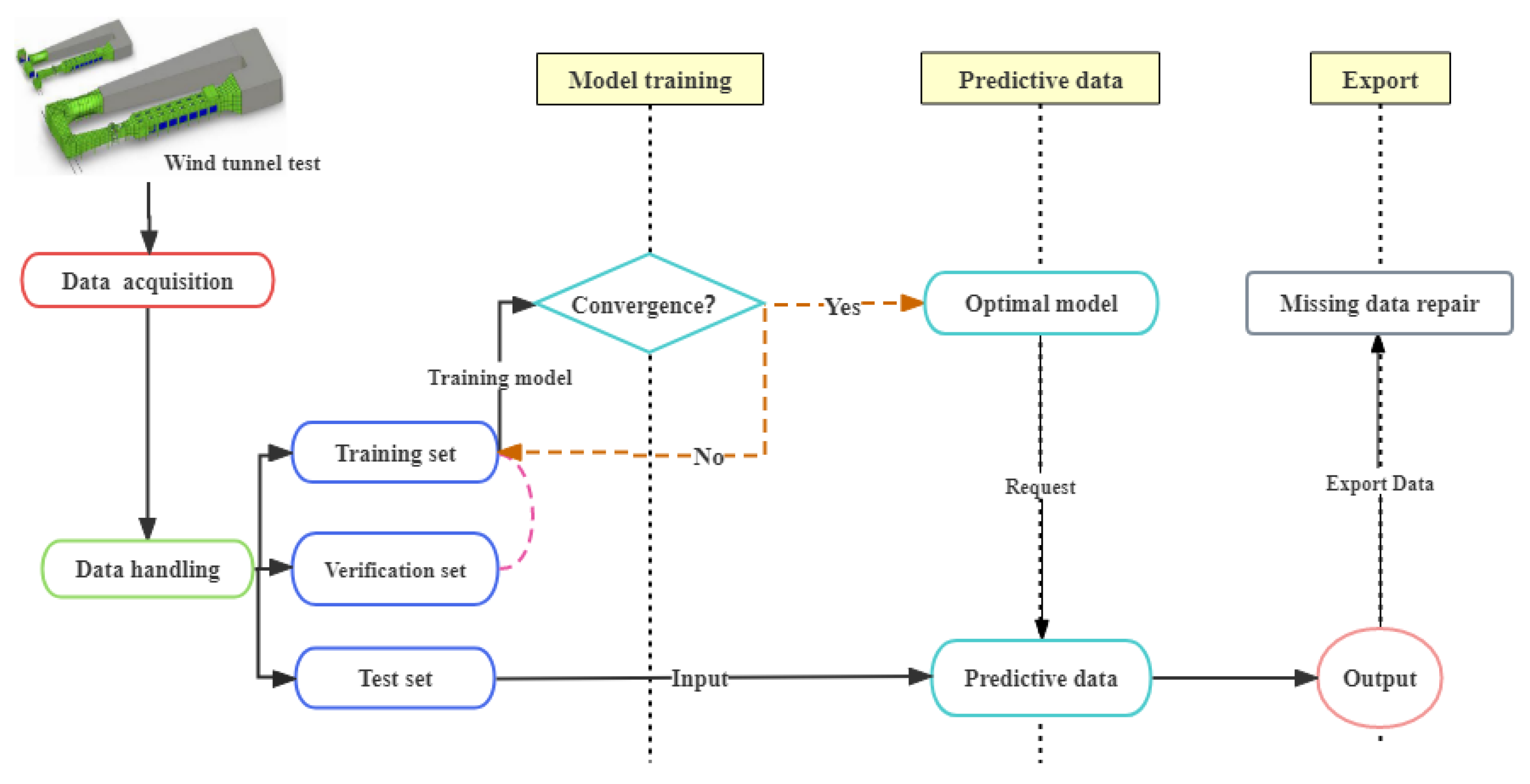
3. Prediction Method of the Wind-Induced Strain Response of Lightning Rod Structures Based on LSTM

Because the strain response between each measurement point of the lightning rod structure has a certain degree of nonlinear mapping relationship [38,39,40], the LSTM network has strong applicability for addressing this problem. Therefore, this paper adopts the LSTM network to repair and predict the missing or defective data of wind-induced dynamic response in the process of testing or monitoring lightning rod structures under different wind speeds. The specific process is shown in Figure 4.

First, the parameters of the LTSM model are optimized by using the strain time-history data of each measurement point of the aeroelastic model of the lightning rod structure obtained from the wind tunnel test, and the most suitable model structure is determined. Then, normal data are used to repair the disease data or “missing” data to ensure the integrity of the data chain. The detailed step descriptions are as follows:

Step 1: Classify the collected dynamic strain test data of 10 measurement points on the strong axis and weak axis of the lightning rod structure. Then, take the first 70% of the data of some measurement points as the training set and the last 30% of the data as the test set. Here, the test set data are treated as “missing” data.

Step 2: Perform noise reduction processing on the collected dataset to reduce the interference of the noise data collected during the test on capturing the nonlinear mapping relationship between the strains of each measurement point. At the same time, the data are normalized to decimals between 0 and 1 to speed up model iteration.

Step 3: Input a part of the data into the model for parameter-seeking training and determine the unknown parameters such as the number of hidden layers, the number of hidden units, and the number of iterations of the model so that the model can reach the optimal structure for the next step of data fitting and prediction.

Step 4: Input the dynamic strain data of the lowest two points of the lightning rod aeroelastic model structure into the sequence X₁ = (x₁, x₂, x₃, …, x_T), X₂ = (x₁, x₂, x₃, …, x_T) and set the dynamic strain sequence of the point to be measured as Y = (y₁, y₂, y₃, …, y_n), that is, using many-to-one model construction. Then, the first 70% of the data (i.e., 0.7T × (M + 1)) of these sequences are used to form a multidimensional matrix [X₁, X₂, …, Y] ^T to perform the machine learning process. Here, M is the number of X vectors, and T is the number of data contained in each column of X vectors.

Step 5: After the model has captured the nonlinear relationship between X₁, X₂… and Y to a considerable extent, the error loss image of the training process is used to judge whether the training is complete and whether the number of iterations is sufficient. If the training error loss image no longer decreases, go to step 6. If the image is still not completely decreased within the limited number of iterations, the number of iteration steps needs to be increased, and step 4 is repeated.

Step 6: Input the last 30% of strain data into the model to predict the Y sequence and then denormalize it to obtain the final predicted value of Y.

Step 7: Take the obtained predicted value Y as the new input value X₃, together with the previous input values X₁ and X_2, to compose a new input matrix [X₁, X₂, X₃]^T. The dynamic strain value of the next adjacent measurement point is used as new “missing” data to predict the value of Y, and steps S2 to S5 are repeated.

Step 8: Repeat steps S2 to S7 to predict the time-history data of the “missing” strain response data of the lightning rod structure.

By comparing the lightning rod strain response time-history data obtained in the above steps with the strain response time-history data actually measured by the wind tunnel test, the accuracy of the prediction results can be judged. On this basis, the average relative error of multiple prediction results is used as the final evaluation indicator for the prediction model.

4. Example Verification

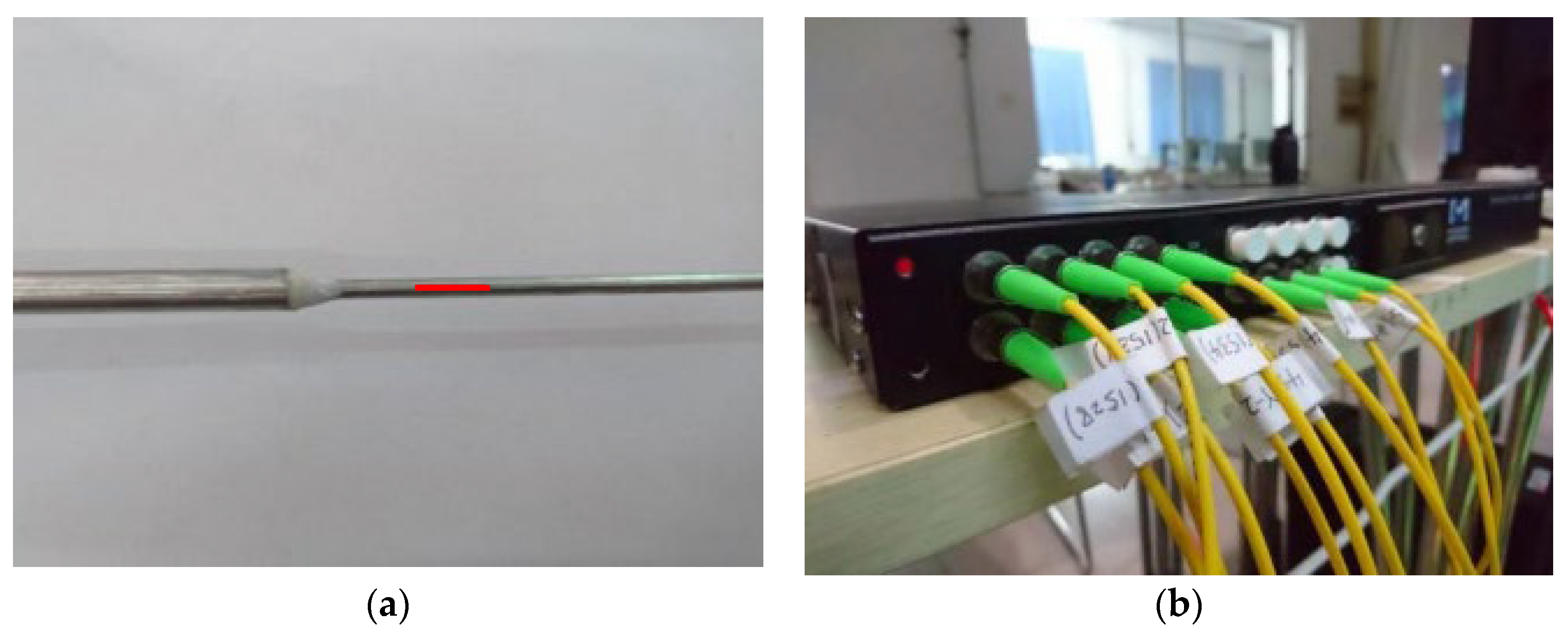
4.1. Wind Tunnel Test of the Lightning Rod Aeroelastic Model

To study the wind-induced vibration response characteristics of frame–lightning rod structures, the research group designed and carried out a wind tunnel test of the scaled aeroelastic model of typical frame lightning rods [1]. Through the wind tunnel test and fiber grating (FBG) strain measurement technology, the strain response time-history of the lightning rod structure aeroelastic model under different wind speeds and different wind directions was measured.

The central wind tunnel during the test is a series double test section return/DC boundary layer wind tunnel with a height 3.0 m and length 24.0 m. According to the design theory of aeroelastic models, combined with the structure type of the lightning rods, the similarity ratios that should be satisfied in the design of the lightning rod aeroelastic model include the geometric ratio, mass ratio, Froude number, Cauchy number, dimensionless frequency, and damping ratio. The similar design parameters used in the aeroelastic model wind tunnel test are shown in

Table 1. Similarity parameters for the aeroelastic model wind tunnel test (n = 1:10).

Similarity Parameter	Geometric Ratio λL	Mass Ratio λM	Wind Speed Ratio λU	Flexural Rigidity Ratio λEI	Frequency Ratio λf	Damping Ratio λζ
Similitude ratio	n	n3	n0.5	n5	n−0.5	1
Values	1:10	1:1000	1:3.16	1:100,000	3.16:1	1

, and the arrangement of one of the models and the strain measurement points of the FBG sensors is shown in Figure 5.

The lightning rod aeroelastic model consists of five sections of rods with different specifications, which are defined as the first section, the second section, the third section, the fourth section and the fifth section from top to bottom. Measurement points are arranged at the center of each segment bottom to measure the strain values of the corresponding measurement points. The side corresponding to the smaller stiffness of the rod is called the weak axis, which is represented by W. The side with the larger stiffness of the rod is called the strong axis, which is represented by S. The W-axis measurement points from top to bottom are W-1, W-2, W-3, W-4, and W-5, and the S-axis measurement points from top to bottom are S-1, S-2, S-3, S-4, and S-5, respectively, as shown in Figure 5b.

Due to the slender and highly flexible structure of lightning rod aeroelastic models, light-weight and small-volume sensors are more suitable for wind tunnel tests to avoid excessive influence on the dynamic response of the model and minimize the measurement error. Therefore, FBG strain sensors are adopted in the experiment to measure the strain value at different measurement points of the structure. Figure 6 shows the location of specific FBG measurement points on the model and the FBG demodulator used in the test.

During the test, the definition of the wind direction angle is shown in Figure 7. The 0° wind direction angle is the case where the windward side is along the W-axis, and the 90° wind direction angle is the case where the windward side is along the S-axis. Under a 0° wind direction angle, the along-wind vibration response measurement points are located on the W-axis, and the crosswind vibration response measurement points are located on the S-axis. The wind speeds during the wind tunnel test are 5 m/s, 6 m/s, 8 m/s, and 10 m/s. According to the similarity ratio of the scaled model, the actual wind speeds of the corresponding lightning rod structure are 15.81 m/s, 18.97 m/s, 25.30 m/s, and 31.62 m/s. The above wind speed range not only includes the main wind speed range when the actual lightning rods work but also includes the extreme wind speed conditions that may occur in practice. For the convenience of guiding engineering practice, in the subsequent analysis, the wind speeds considered in this study are expressed in accordance with the actual wind speeds.

4.2. Selection and Processing of Data Samples

The strain values at the ten measurement points under the action of four different wind speeds (i.e., 15.81 m/s, 18.97 m/s, 25.30 m/s, 31.62 m/s) were sampled. The sampling frequency and time were 250 Hz and 40 s, respectively. There were 40 samples in total, and each sample contained 10,000 strain values. The first 70% of all the samples was used to train the LTSM network model. The remaining 30% of the data in the sample set of measurement points 1 to 3 were regarded as the “missing” data to test the LTSM network model. The evaluation indices [41,42] of the model were the root mean square error (RMSE), the mean absolute error (MAE), the variance accounted for (VAF) and the refined Willmott index (RWI). When the values of VAF and RWI are close enough to 1 and the values of RMSE and MAE are close enough to 0, the LSTM model can be considered excellent. The formulas for calculating the abovementioned indices were as follows:

$$\mathrm{RMSE}=\sqrt{\frac{1}{n}{\displaystyle {\sum }_{\mathrm{i}=1}^{\mathrm{n}}(y_{\mathrm{i}}-y_{\mathrm{it}}{)}^2}}$$

(9)

$$\mathrm{MAE}=\frac{1}{n}{\displaystyle {\sum }_{\mathrm{i}=1}^{\mathrm{n}}{\left|y_{\mathrm{i}}-y_{\mathrm{it}}\right|}^{}}$$

(10)

$$\mathrm{VAF}=1-\frac{\mathrm{var}(y_{\mathrm{i}}-y_{\mathrm{it}})}{\mathrm{var}(y_{\mathrm{i}})}$$

(11)

$$\mathrm{RWI}=1-\frac{{\displaystyle \sum _{\mathrm{i}=1}^{\mathrm{n}}\left|y_{\mathrm{i}}-y_{\mathrm{it}}\right|}}{2{\displaystyle \sum _{\mathrm{i}=1}^{\mathrm{n}}\left|y_{\mathrm{i}}-y_{\mathrm{n}}\right|}}$$

(12)

In Formulas (9) to (12), n is the number of test samples, y_i is the measured value at time i, y_it is the predicted value at time i, var represents variance, and y_n is the average value of the measured samples.

Meanwhile, the data in the training set and test set can also be normalized to improve the prediction accuracy and prediction speed. The calculation formula for normalization is:

$$x_{\mathrm{norm}}=\frac{x-m_{\mathrm{ean}}}{v_{\mathrm{ariance}}}$$

(13)

In Formula (13), m_ean is the mean of the input samples, and v_ariance is the variance of the input samples.

Take, as an example, the lightning rod under the action of wind speed 25.30 m/s. A total of 30,000 data points were selected from the test values of measurement points S-3, S-4, and S-5 on the strong axis to train and optimize the LTSM network model parameters. The data of measurement points S-4 and S-5 are used as the input data, and the data of measurement point S-3 are used as the output data. The measured time-history strain values of the abovementioned measurement points during the wind tunnel test are demonstrated in Figure 8.

Figure 8 shows that the time-history data fluctuate greatly in the first 5 s after the start of the test, and the difference is obvious from the data after that. To make the optimization of the model parameters more accurate and to minimize the adverse effect of noise data on the predictive results, the measured data of the first 5 s are removed, and the data from 5 s to 45 s are used for simulation and prediction in the subsequent analysis. The updated time-history data are shown in Figure 9.

4.3. Determination of Model Structure and Parameters

MATLAB 2018a deep learning tools were used to build the predictive models. Due to the large number and the high dimensions of the measured data, a dropout layer is adopted to prevent the model from overfitting during the learning process. During analysis, the parameters of the LSTM model are first determined, and then the influence of different LSTM layers and hidden units on the prediction results is studied to find the optimal model parameters, and the basic control variable method is used for analysis.

To ensure that the model fully captures the nonlinear mapping relationship between the data, the number of iterations is set to 1000, and the initial learning rate is 0.005. The range of the number of hidden layers is set to 1 to 7, and the range of the number of hidden units is set to between 50 and 600, with a value interval of 50. The two independent variables (i.e., number of hidden layers and number of hidden units) are simulated, and the final fitting result of the three-dimensional surface graph is shown in Figure 10a. At the same time, to determine the most suitable number of iterations, the root mean square error (RMSE) of the test set during the training process of the LSTM neural network is counted, and its descending curve is shown in Figure 10b.

From Figure 10a, it can be observed that the RMSE values change with the number of hidden layers and the number of hidden units. When the number of hidden layers is 3, the RMSE value is stable between 0.45 and 0.5, and the error is small compared to other combinations of hidden layers and hidden units. Figure 10b indicates that when the number of iterations is approximately 1000, the RMSE gradually tends to be stable. Since the calculation time of the model is positively correlated with the number of hidden layers, the number of hidden units and the number of iterations, to obtain the best balance between the calculation time and the calculation results, the optimal number of hidden units is set to 250, and the number of iterations is set to 1000.

The LSTM neural network model established in this paper includes an input layer for receiving input data; three LSTM layers for modeling the data; three dropout layers, with the dropout rate set to 0.2 to prevent data from being overfitted; and an FC layer for dimensional transformation of the output data.

The Adam optimizer is used in the neural network training process, the threshold activation function is the σ function, the output activation function is the tanh function, and the initial learning rate is 0.005. The maximum number of iterations is set to 1000. The dynamic learning rate is adopted, and the learning rate is reduced by half after every 500 training iterations. At the same time, the weight parameters of the LSTM model are normalized to prevent data from being overfitted. The parameter for normalization is set to 0.01. At this point, the neural network parameter training is complete, and the final optimal network parameters are presented in

Table 2. LSTM network parameters.

Layer	Type	Activation Function	Output Shape
Input	InputLayer	-	(none, n, f + 1)
LSTM1	LSTM	tanh	(none, n, 250)
Dropout1	dropout	-	0.2
LSTM2	LSTM	tanh	(none, n, 250)
Dropout2	dropout	-	0.2
LSTM3	LSTM	tanh	(none, n, 250)
Dropout3	dropout	-	0.2
FC	Dense	Linear	(none, s × f)

Note: n is the length of the input time series; s is the length of the output time series; f is the number of degrees of freedom for prediction.

.

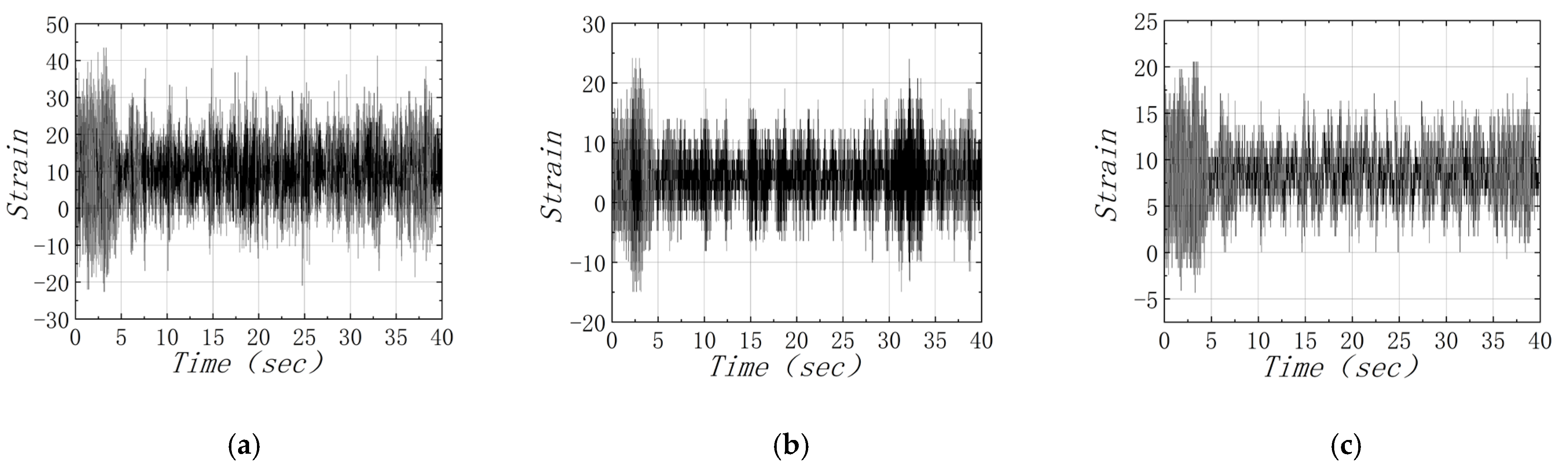
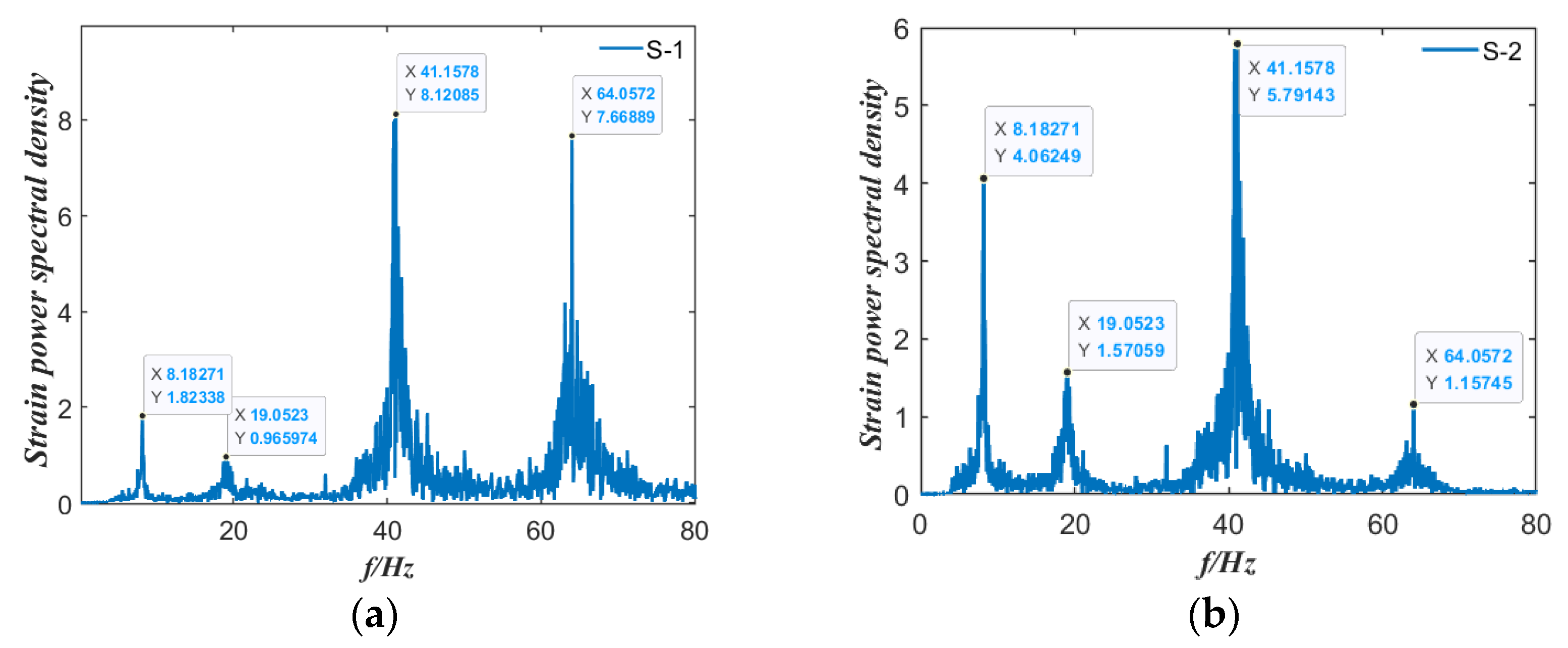
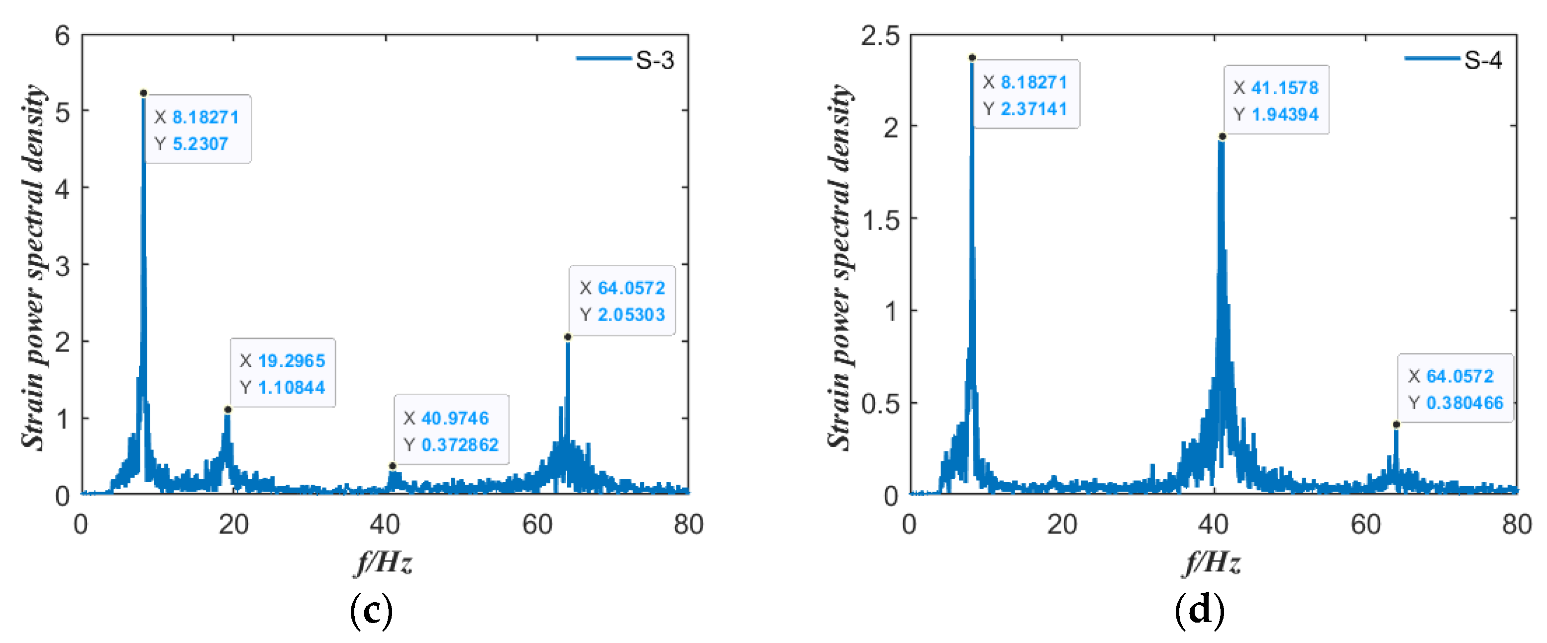
4.4. Analysis of Wind Vibration Response of Lightning Rod Structure under the Action of Wind Speed 25.30 m/s

The first four orders of modal frequencies of the lightning rod aeroelastic model structure are shown in

Table 3. The first four orders of vibration mode frequencies of the lightning rod aeroelastic model.

Modal Number	Aeroelastic Model Natural Frequency (Hz)
	W-Axis	S-Axis
1st order	7.95	8.97
2nd order	17.48	19.23
3rd order	43.41	47.49
4th order	64.02	71.84

. To find the weak parts of the lightning rod structure and identify the positions where the sensors are more likely to damage and cause data loss or drift during the test process, a Fourier transform of the strain time-history under 25.3 m/s wind speed and 0 degree wind direction angle is performed. The along-wind and crosswind vibration strain power spectra of the four measurement points on the upper part of the structure are shown in Figure 11 and Figure 12, respectively.

Figure 11 shows that the along-wind vibration characteristic of the upper part near the W-1 measurement point of the lightning rod is the most complex; its vibration response contains the mode components of the first four orders, with corresponding frequencies of 7.51099 Hz, 17.7699 Hz, 38.9595 Hz, and 64.0572 Hz. The vibration response of the structure near measurement point W-2 mainly includes the first-, second- and third-order mode components, while the vibration response of the structure near measurement point W-3 is dominated by the contribution of the first- and second-order modes. By and large, the high-frequency vibration response of the lightning rod structure mainly occurs in the upper part of the structure, the vibration is jointly controlled by multiple modes of vibration, and the vibration amplitude becomes stronger with increasing wind speed, while the vibration of the lower part of the structure is basically dominated by the contribution of the fundamental vibration mode. Therefore, the sensors at the upper part of the lightning rod structure are more prone to damage, resulting in data loss or abnormality.

Figure 12 also shows that the crosswind vibration characteristic of the structure near the upper measurement points is relatively complex, and its vibration response contains mode components of the first four orders. The corresponding modal frequencies are 8.18271 Hz, 19.0523 Hz, 41.1578 Hz, and 64.0572 Hz. Under a wind speed of 25.30 m/s, the high-frequency vibration of the lightning rod near measurement point S-1 is the most severe, which also indicates the position where exceptional monitoring data are prone to occur during the test.

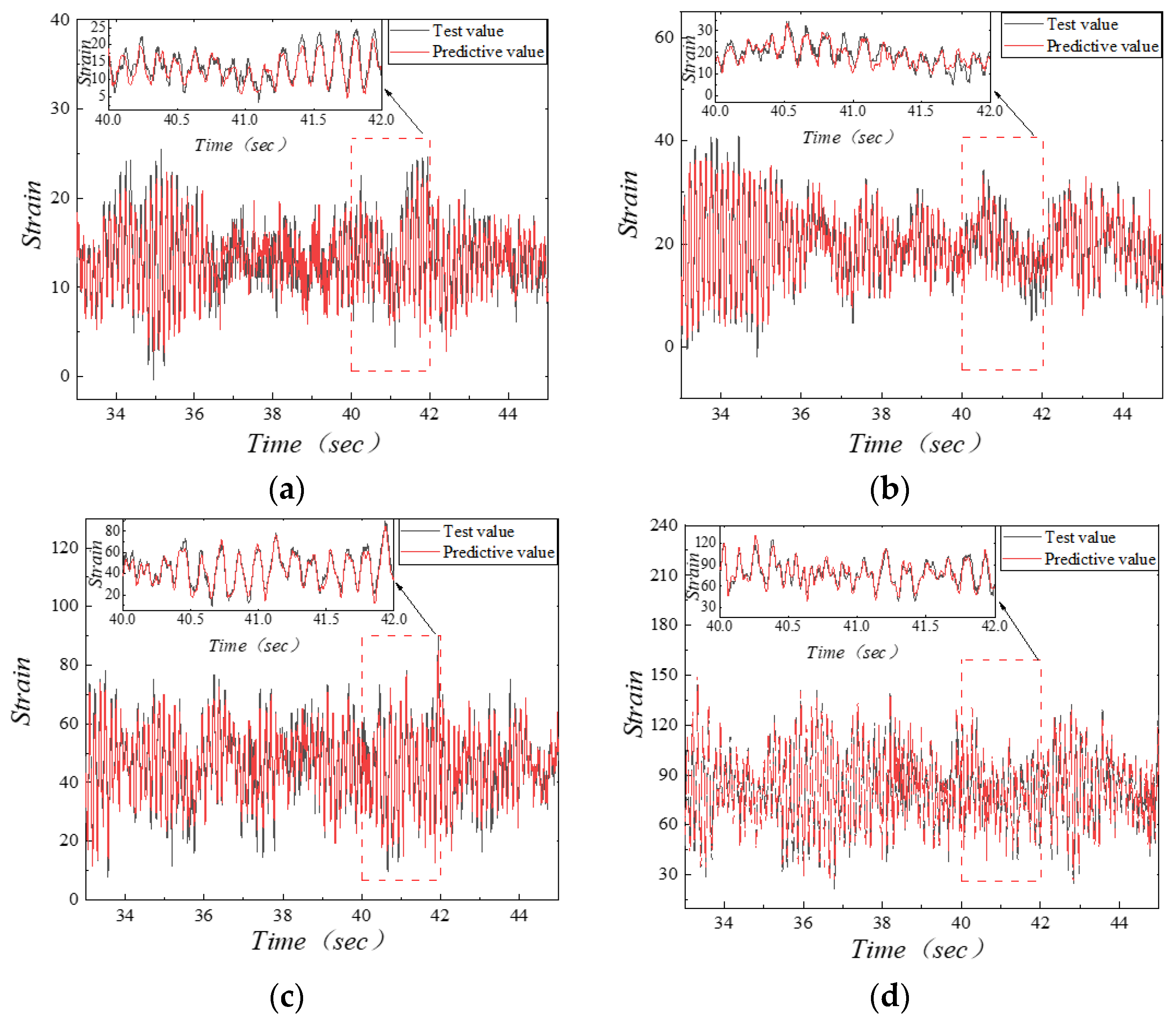
4.5. Prediction Results of the Strain Response Data of the Lightning Rod

Based on the LSTM neural network model trained in the previous sections, the along-wind and crosswind strain response data of measurement points 1 to 5 of the lightning rod under different wind speeds are adopted to predict the “missing” strain response. Here, the measured strain response data of measurement points 4 and 5 are used as input data, and the strains of measurement points 1, 2 and 3 are treated as output data. Using the simulation method proposed in the above sections, the along-wind and crosswind strain response data are predicted, and the results are shown in Figure 13, Figure 14, Figure 15, Figure 16, Figure 17 and Figure 18.

Figure 13, Figure 14, Figure 15, Figure 16, Figure 17 and Figure 18 show that the strain time-history responses at each measurement point predicted by the LSTM model are in good agreement with the measured values by the wind tunnel test, regardless of whether under frequently encountered wind speed or extreme wind speed conditions, indicating that the proposed method in this paper has high reliability and stability.

In practical engineering, the vibration amplitude of a lightning rod usually increases with increasing wind speed, which may cause damage to the sensors on the upper part of the structure under extreme wind speed conditions, resulting in measured data abnormities or broken data chains. Therefore, it is more meaningful to accurately predict the vibration response of the structure under the condition of high wind speed.

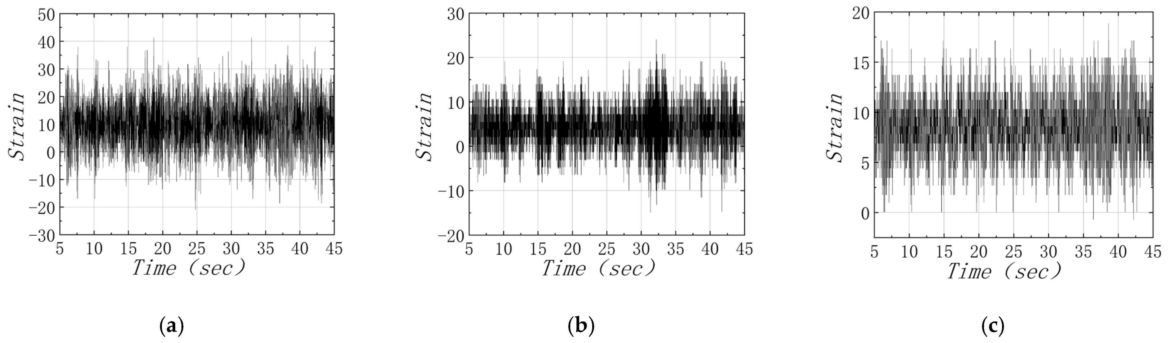
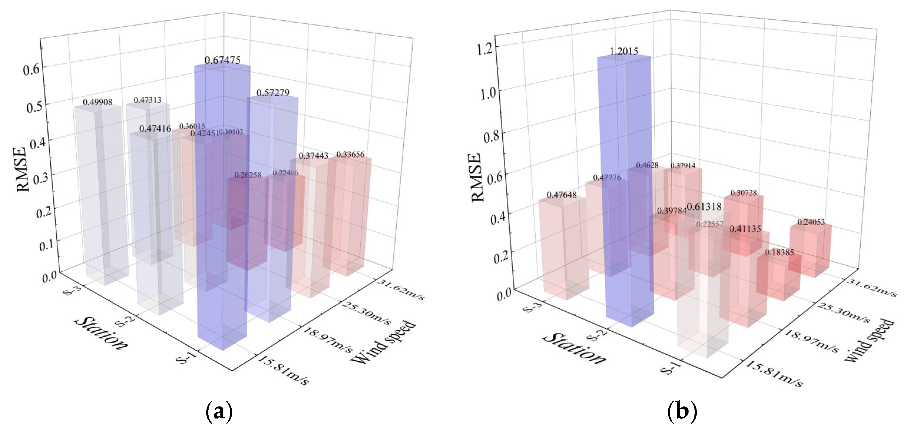
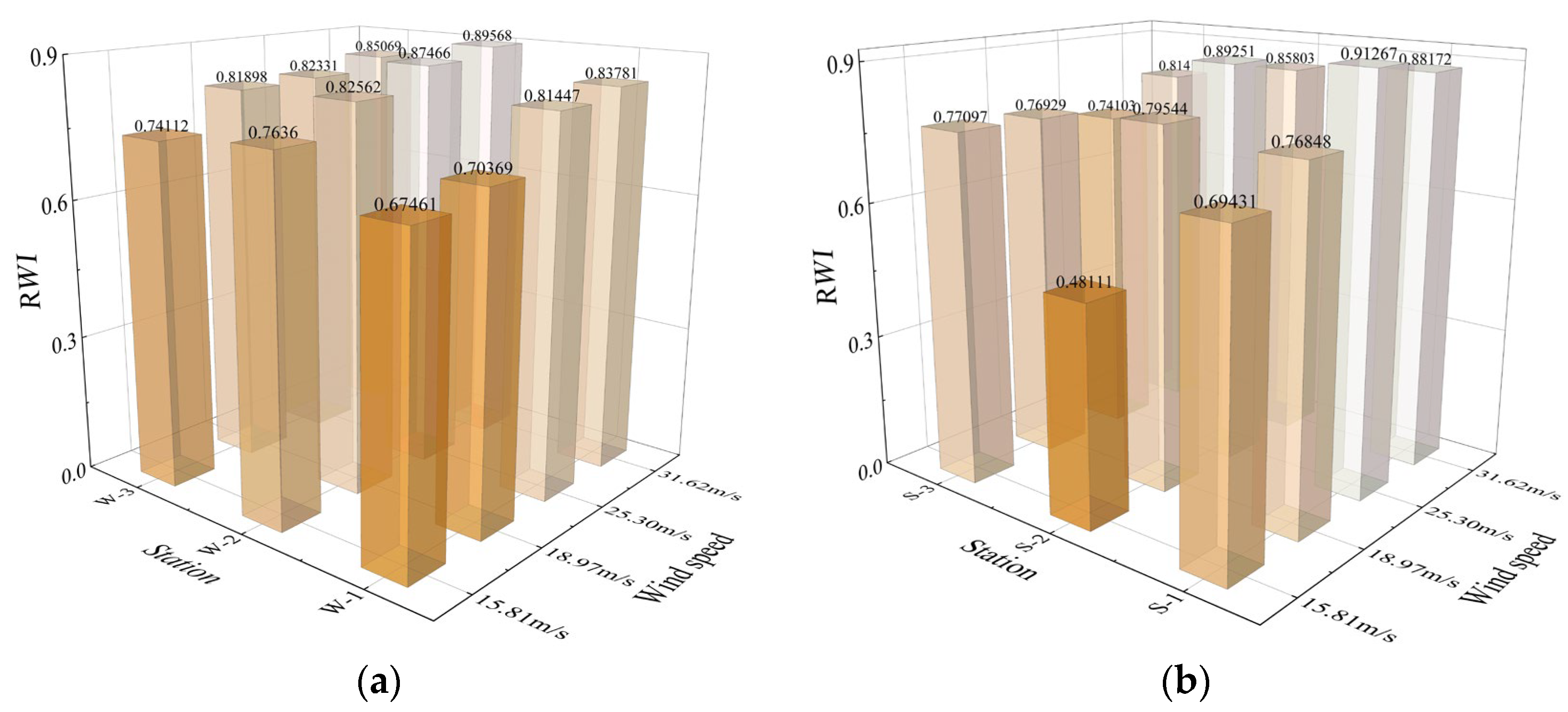
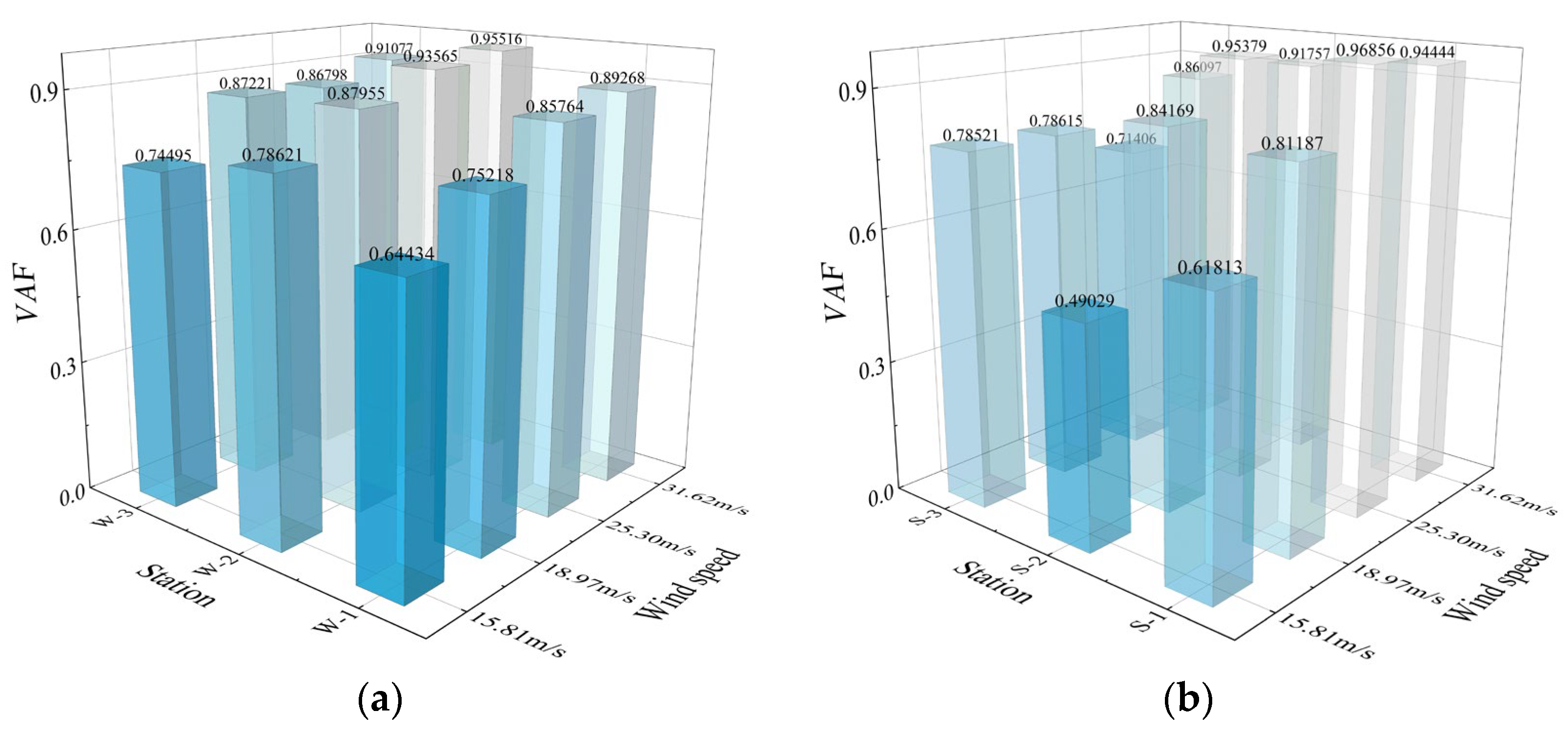
4.6. Correlation Analysis of the Predictive Data under Extreme Wind Speed Conditions

The above analysis shows that the structural vibration response is most complex and strongest at measurement points W-1 and S-1 under the extreme wind speed 31.62 m/s. The sensors in these positions are most likely to fail in actual engineering, resulting in an incomplete response data chain. To identify whether the proposed prediction method can meet the needs of engineering applications, a correlation analysis of the predictive data under extreme wind speed conditions is performed in this study, and the results are shown in Figure 19. Here, R² is the coefficient of determination, and the range of its value is 0 to 1. Moreover, the closer the value of R² is to 1, the better the data prediction effect.

It can be seen from Figure 19 that even under extreme wind speed conditions, the coefficient of determination of the predicted data at the most unfavorable position of the lightning rod (i.e., measurement point 1) is approximately 0.9, and the predicted and measured values are evenly distributed on both sides of the fitting curve. There is no abnormal drift point, indicating that the prediction ability of the model in this paper has a high guarantee rate and can meet the actual engineering needs. At the same time, with the help of the unique data feature importance analysis function of the random forest method, the weight coefficients of different input data features for the prediction results can be obtained. When predicting the “missing” data at monitoring point 1, four sets of measured data from measurement point 2 to measurement point 5 were used, and the final analysis results are shown in Figure 20.

Figure 20 shows that when predicting the strain response of the lightning rod at measurement point S-1, the measured data at measurement point S-2 play a decisive role in the predictive results at measurement point S-1, and its weight coefficient reaches 0.48. The influence of the data of measurement point S-3 on the prediction results of measurement point S-1 is second only to that of measurement point S-2, and its weight coefficient is 0.23. The influence of the data of measurement point S-5 and measurement point S-4 on the prediction results is basically similar, and their weight coefficients are approximately 0.15. In general, the measured response data of the monitoring points that are closer to the predicted measurement point have a greater impact on the response of the predicted measurement point, while the measured response data of monitoring points that are far from the predicted measurement point have less impact on the response of the predicted measurement point and are considered ignorable. To compare the precision of the prediction results of each working condition analyzed in this paper more intuitively, the RMSE, MAE, RWI and VAF of the prediction results corresponding to each working condition are also analyzed, and the results are shown in Figure 21, Figure 22, Figure 23 and Figure 24.

Figure 21 and Figure 22 show that within the wind speed range analyzed in this paper, the RMSE and MAE values of the prediction results of each measurement point on the W-axis of the lightning rod show a negative correlation as a whole with the increase in wind speed, and under the same wind speed conditions, the RMSE and MAE values of each measurement point are relatively stable.

Figure 23 and Figure 24 indicate that within the wind speed range analyzed in this paper, the RWI and VIF values of each measurement point of the lightning rod structure gradually increase with increasing wind speed and finally tend to 1. On the S-axis side of the lightning rod, when the wind speed is 25.30 m/s, the prediction precision of the response results of measurement point S-1 is the highest. For other measurement points on the S-axis, the prediction precision can still reach an excellent level, which shows that the LSTM model built in this paper has a certain degree of generalization capability.

5. Conclusions

This paper proposes a method based on an LSTM neural network to predict the “missing” response data of lightning rod structures under wind-induced vibration. The prediction of the “missing” strain value of each measurement point in the along-wind and crosswind directions of the lightning rod under different wind speeds is carried out, and the random forest method is used to analyze the correlation relationship between the predicted data and the measured data under extremely high wind speed conditions. The main conclusions are as follows:

• The high-frequency and complex response of the lightning rod structure in the along-wind direction and the crosswind direction mainly occurs near measurement point 1 on the upper part of the structure. Problems such as loss or abnormality of monitoring data are prone to occur. Therefore, it is important to focus on this measurement point and prepare for missing data prediction during testing and monitoring.
• Under the normal working wind speed range of the lightning rod structure, regardless of whether frequently encountered wind speed or extreme wind speed, the strain responses of the measurement point predicted by the LSTM model are in good agreement with the measured values of the wind tunnel test. Even under the case of an extreme wind speed of 31.62 m/s, the values of RMSE, MAE, R², RWI and VAF are 0.24053, 0.18213, 0.94539, 0.88172 and 0.94444, respectively, which are within the acceptable range, indicating that the LSTM method can better capture the nonlinear mapping relationship between the strains of each measurement point and has high reliability and stability.
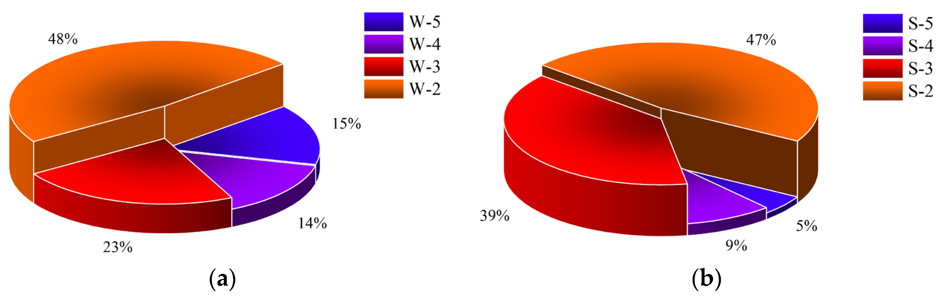
• In the structural vibration response prediction, measurement point 2 plays a decisive role in the prediction result at measurement point 1, while the influence of measurement points 5 and 4 on the prediction results is almost negligible. In general, the measured response data of the monitoring points that are closer to the predicted measurement point have a greater impact on the response of the predicted measurement point, while the measured response data of monitoring points that are far from the predicted measurement point have less impact on the response of the predicted measurement point and are considered ignorable.
• Finally, it should be noted that it is necessary to perform more complex processing on the noise data to make the prediction results more accurate and meet engineering requirements.

References

1. Zhao, G.; Li, J.; Zhang, M.; Yi, Y. Experimental study on the bearing capacity and fatigue life of lightning rod structure joints in high-voltage substation structures. Thin-Walled Struct. 2022, 175, 109282. [Google Scholar] [CrossRef]
2. Guojun, D.; Lei, G.; Manling, D. Break Fault Analysis and Countermeasure of Frame Lighting Rod. Henan Electr. Power 2015, 4, 6–9. [Google Scholar]
3. Tao, S. A Cause Analysis of Fracture Failure with Architecture Type Lightning Rod. Insul. Surge Arresters 2017, 2, 49–52. [Google Scholar]
4. Jian, W.; Heming, D. The Deformation Analysis and Countermeasures on the Frame Lightning Rod of 750 kV Substation in the Wind Damage Areas. Insul. Surge Arresters 2017, 2, 14–18. [Google Scholar]
5. Gomez-Cabrera, A.; Escamilla-Ambrosio, P.J. Review of Machine-Learning Techniques Applied to Structural Health Monitoring Systems for Building and Bridge Structures. Appl. Sci. 2022, 12, 10754. [Google Scholar] [CrossRef]
6. Ye, X.W.; Jin, T.; Yun, C.B. A review on deep learning-based structural health monitoring of civil infrastructures. Smart Struct. Syst. 2019, 24, 567–585. [Google Scholar]
7. Rucevskis, S.; Kovalovs, A.; Chate, A. Optimal Sensor Placement in Composite Circular Cylindrical Shells for Structural Health Monitoring. J. Phys. Conf. Ser. 2023, 2423, 12021. [Google Scholar] [CrossRef]
8. Luo, Y.; Mei, Y.; Shen, Y.; Yang, P.; Jin, L.; Zhang, P. Field measurement of temperature and stress on steel structure of the National Stadium and analysis of temperature action. J. Build. Struct. 2013, 34, 24–32. [Google Scholar]
9. Amezquita-Sanchez, J.P.; Valtierra-Rodriguez, M.; Adeli, H. Wireless smart sensors for monitoring the health condition of civil infrastructure. Sci. Iran. 2018, 25, 2913–2925. [Google Scholar]
10. Sabato, A.; Niezrecki, C.; Fortino, G. Wireless MEMS-based accelerometer sensor boards for structural vibration monitoring: A review. IEEE Sens. J. 2016, 17, 226–235. [Google Scholar] [CrossRef]
11. Sarkar, S.; Reddy, K.K.; Giering, M. Deep learning for structural health monitoring: A damage characterization application. In Proceedings of the Annual Conference of the PHM Society, Denver, CO, USA, 3–6 October 2016; Volume 8. [Google Scholar]
12. Oh, B.K.; Glisic, B.; Kim, Y.; Park, H.S. Convolutional neural network-based data recovery method for structural health monitoring. Struct. Health Monit. 2020, 19, 1821–1838. [Google Scholar] [CrossRef]
13. Muin, S.; Mosalam, K.M. Structural health monitoring using machine learning and cumulative absolute velocity features. Appl. Sci. 2021, 11, 5727. [Google Scholar] [CrossRef]
14. Yuen, K.V.; Kuok, S.C. Ambient interference in long-term monitoring of buildings. Eng. Struct. 2010, 32, 2379–2386. [Google Scholar] [CrossRef]
15. Cross, E.J.; Manson, G.; Worden, K.; Pierce, S.G. Features for damage detection with insensitivity to environmental and operational variations. Proc. R. Soc. A Math. Phys. Eng. Sci. 2012, 468, 4098–4122. [Google Scholar] [CrossRef]
16. Sarmadi, H.; Karamodin, A. A novel anomaly detection method based on adaptive Mahalanobis-squared distance and one-class kNN rule for structural health monitoring under environmental effects. Mech. Syst. Signal Process. 2020, 140, 106495. [Google Scholar] [CrossRef]
17. Padil, K.H.; Bakhary, N.; Abdulkareem, M.; Li, J.; Hao, H. Nonprobabilistic method to consider uncertainties in frequency response function for vibration-based damage detection using artificial neural network. J. Sound Vib. 2020, 467, 115069. [Google Scholar] [CrossRef]
18. Bao, Y.; Tang, Z.; Li, H.; Zhang, Y. Computer vision and deep learning–based data anomaly detection method for structural health monitoring. Struct. Health Monit. 2019, 18, 401–421. [Google Scholar] [CrossRef]
19. Tang, Z.; Chen, Z.; Bao, Y.; Li, H. Convolutional neural network-based data anomaly detection method using multiple information for structural health monitoring. Struct. Control Health Monit. 2019, 26, e2296. [Google Scholar] [CrossRef]
20. Avci, O.; Abdeljaber, O.; Kiranyaz, S.; Hussein, M.; Inman, D.J. Wireless and real-time structural damage detection: A novel decentralized method for wireless sensor networks. J. Sound Vib. 2018, 424, 158–172. [Google Scholar] [CrossRef]
21. Hochreiter, S.; Schmidhuber, J. Long short-term memory. Neural Comput. 1997, 9, 1735–1780. [Google Scholar] [CrossRef]
22. Li, S.; Li, S.; Laima, S.; Li, H. Data-driven modeling of bridge buffeting in the time domain using long short-term memory network based on structural health monitoring. Struct. Control Health Monit. 2021, 28, e2772. [Google Scholar] [CrossRef]
23. Sherstinsky, A. Fundamentals of recurrent neural network (RNN) and long short-term memory (LSTM) network. Phys. D Nonlinear Phenom. 2020, 404, 132306. [Google Scholar] [CrossRef]
24. Iparraguirre-Villanueva, O.; Alvarez-Risco, A.; Salazar, J.L.H.; Beltozar-Clemente, S.; Zapata-Paulini, J.; Yáñez, J.A.; Cabanillas-Carbonell, M. The Public Health Contribution of Sentiment Analysis of Monkeypox Tweets to Detect Polarities Using the CNN-LSTM Model. Vaccines 2023, 11, 312. [Google Scholar] [CrossRef] [PubMed]
25. Smagulova, K.; James, A.P. A survey on LSTM memristive neural network architectures and applications. Eur. Phys. J. Spec. Top. 2019, 228, 2313–2324. [Google Scholar] [CrossRef]
26. Bakhshi Ostadkalayeh, F.; Moradi, S.; Asadi, A.; Nia, A.M.; Taheri, S. Performance Improvement of LSTM-based Deep Learning Model for Streamflow Forecasting Using Kalman Filtering. Water Resour. Manag. 2023, 1–17. [Google Scholar] [CrossRef]
27. Chen, X.; Chen, W.; Dinavahi, V.; Liu, Y.; Feng, J. Short-Term Load Forecasting and Associated Weather Variables Prediction Using ResNet-LSTM Based Deep Learning. IEEE Access 2023, 11, 5393–5405. [Google Scholar] [CrossRef]
28. Graves, A.; Schmidhuber, J. Framewise phoneme classification with bidirectional LSTM and other neural network architectures. Neural Netw. 2005, 18, 602–610. [Google Scholar] [CrossRef]
29. Liu, H.-J.; Shan, W.-F.; Geng, G.-Z. Earthquake Prediction Using Dissolved Radon Data in Long and Short Term Memory Network. Sci. Technol. Eng. 2020, 20, 4029–4035. [Google Scholar]
30. Gers, F.A.; Schmidhuber, J.; Cummins, F. Learning to forget: Continual prediction with LSTM. Neural Comput. 2000, 12, 2451–2471. [Google Scholar] [CrossRef]
31. Nasir, J.; Aamir, M.; Haq, Z.U.; Khan, S.; Amin, M.Y.; Naeem, M. A new approach for forecasting crude oil prices based on stochastic and deterministic influences of LMD Using ARIMA and LSTM Models. IEEE Access 2023, 11, 14322–14339. [Google Scholar] [CrossRef]
32. De Pater, I.; Mitici, M. Developing health indicators and RUL prognostics for systems with few failure instances and varying operating conditions using a LSTM autoencoder. Eng. Appl. Artif. Intell. 2023, 117, 105582. [Google Scholar] [CrossRef]
33. Roux, A.; Changey, S.; Weber, J.; Lauffenburger, J.-P. LSTM-Based Projectile Trajectory Estimation in a GNSS-Denied Environment. Sensors 2023, 23, 3025. [Google Scholar] [CrossRef] [PubMed]
34. Zhang, R.; Chen, Z.; Chen, S.; Zheng, J.; Büyüköztürk, O.; Sun, H. Deep long short-term memory networks for nonlinear structural seismic response prediction. Comput. Struct. 2019, 220, 55–68. [Google Scholar] [CrossRef]
35. Byeon, W.; Breuel, T.M.; Raue, F.; Liwicki, M. Scene labeling with lstm recurrent neural networks. In Proceedings of the IEEE Conference on Computer Vision and Pattern Recognition, Boston, MA, USA, 7–12 June 2015; pp. 3547–3555. [Google Scholar]
36. Long, X.; Ding, X.; Li, J.; Dong, R.; Su, Y.; Chang, C. Indentation Reverse Algorithm of Mechanical Response for Elastoplastic Coatings Based on LSTM Deep Learning. Materials 2023, 16, 2617. [Google Scholar] [CrossRef]
37. Long, B.; Tan, F.; Newman, M. Forecasting the Monkeypox Outbreak Using ARIMA, Prophet, NeuralProphet, and LSTM Models in the United States. Forecasting 2023, 5, 127–137. [Google Scholar] [CrossRef]
38. Xie, X.; Luo, Y.; Zhang, N. Miss data reconstruction in stress monitoring of steel spatial structures using neural network techniques. Spat. Struct. 2019, 25, 38–44. [Google Scholar]
39. Han, J.; Pak, W. Hierarchical LSTM-Based Network Intrusion Detection System Using Hybrid Classification. Appl. Sci. 2023, 13, 3089. [Google Scholar] [CrossRef]
40. Xu, Z.; Chen, J.; Shen, J.; Xiang, M. Recursive long short-term memory network for predicting nonlinear structural seismic response. Eng. Struct. 2022, 250, 113406. [Google Scholar] [CrossRef]
41. Raja, M.N.A.; Shukla, S.K. Predicting the settlement of geosynthetic-reinforced soil foundations using evolutionary artificial intelligence technique. Geotext. Geomembr. 2021, 49, 1280–1293. [Google Scholar] [CrossRef]
42. Demirbay, B.; Bayram, D.; Uur, A. A bayesian regularized feed-forward neural network model for conductivity prediction of ps/mwcnt nanocomposite film coatings. Appl. Soft Comput. 2020, 96, 106632. [Google Scholar] [CrossRef]
Figure 1. Substation structure and lightning rod structure. (a) A substation. (b) Frame–lightning rod structure.
Buildings 13 01256 g001
Figure 2. Structure diagram of the nth LSTM cell hidden layer at time t.
Buildings 13 01256 g002
Figure 3. Multilayer LSTM structure model diagram.
Buildings 13 01256 g003
Figure 4. Flow chart of LSTM prediction and analysis of the strain value of the lightning rod structure measurement point.
Buildings 13 01256 g004
Figure 5. Aeroelastic model and strain measurement points. (a) Aeroelastic model. (b) Arrangement of the FBG sensor strain measurement points.
Buildings 13 01256 g005
Figure 6. FBG measurement point and FBG demodulator. (a) FBG measurement point (red). (b) FBG demodulator.
Buildings 13 01256 g006
Figure 7. Schematic diagram of the lightning rod wind direction angle.
Buildings 13 01256 g007
Figure 8. Measured strain time-history diagram of the measurement points of S-3, S-4, S-5. (a) Measured strain values at measurement point S-3. (b) Measured strain values at measurement point S-5. (c) Measured strain values at measurement point S-5.
Buildings 13 01256 g008
Figure 9. Updated strain time-history diagram of the measurement points of S-3, S-4, S-5 after noise elimination. (a) Updated strain values at measurement point S-3. (b) Updated strain values at measurement point S-5. (c) Updated strain values at measurement point S-5.
Buildings 13 01256 g009
Figure 10. RMSE values for different parameters. (a) RMSE surface graph under different parameters. (b) Changing of RMSE value during the learning process.
Buildings 13 01256 g010
Figure 11. Along-wind vibration strain power spectrum of each measurement point of the lightning rod under a wind speed of 25.3 m/s. (a) Along-wind strain power spectrum at measurement point W-1. (b) Along-wind strain power spectrum at measurement point W-2. (c) Along-wind strain power spectrum at measurement point W-3. (d) Along-wind strain power spectrum at measurement point W-4.
Buildings 13 01256 g011
Figure 12. Crosswind vibration strain power spectrum of each measurement point of the lightning rod under a wind speed of 25.3 m/s. (a) Strain power spectrum at measurement point S-1. (b) Strain power spectrum at measurement point S-2. (c) Strain power spectrum at measurement point S-3. (d) Strain power spectrum at measurement point S-4.
Buildings 13 01256 g012aBuildings 13 01256 g012b
Figure 13. Comparison of the prediction results and test values of along-wind strain response at W-1 measurement point of the lightning rod under different wind speeds. (a) Strain values at measurement point W-1 under a wind speed of 15.81 m/s. (b) Strain values at measurement point W-1 under a wind speed of 18.97 m/s. (c) Strain values at measurement point W-1 under a wind speed of 25.30 m/s. (d) Strain values at measurement point W-1 under a wind speed of 31.62 m/s.
Buildings 13 01256 g013
Figure 14. Comparison of the prediction results and test values of along-wind strain response at W-2 measurement point of the lightning rod under different wind speeds. (a) Strain values at measurement point W-2 under a wind speed of 15.81 m/s. (b) Strain values at measurement point W-2 under a wind speed of 18.97 m/s. (c) Strain values at measurement point W-2 under a wind speed of 25.30 m/s. (d) Strain values at measurement point W-2 under a wind speed of 31.62 m/s.
Buildings 13 01256 g014
Figure 15. Comparison of the prediction results and test values of along-wind strain response at W-3 measurement point of the lightning rod under different wind speeds. (a) Strain values at measurement point W-3 under a wind speed of 15.81 m/s. (b) Strain values at measurement point W-3 under a wind speed of 18.97 m/s. (c) Strain values at measurement point W-3 under a wind speed of 25.30 m/s. (d) Strain values at measurement point W-3 under a wind speed of 31.62 m/s.
Buildings 13 01256 g015
Figure 16. Comparison of the prediction results and test values of crosswind strain response at S-1 measurement point of the lightning rod under different wind speeds. (a) Strain values at measurement point S-1 under a wind speed of 15.81 m/s. (b) Strain values at measurement point S-1 under a wind speed of 18.97 m/s. (c) Strain values at measurement point S-1 under a wind speed of 25.30 m/s. (d) Strain values at measurement point S-1 under a wind speed of 31.62 m/s.
Buildings 13 01256 g016aBuildings 13 01256 g016b
Figure 17. Comparison of the prediction results and test values of crosswind strain response at S-2 measurement point of the lightning rod under different wind speeds. (a) Strain values at measurement point S-2 under a wind speed of 15.81 m/s. (b) Strain values at measurement point S-2 under a wind speed of 18.97 m/s. (c) Strain values at measurement point S-2 under a wind speed of 25.30 m/s. (d) Strain values at measurement point S-2 under a wind speed of 31.62 m/s.
Buildings 13 01256 g017
Figure 18. Comparison of the prediction results and test values of crosswind strain response at S-3 measurement point of the lightning rod under different wind speeds. (a) Strain values at measurement point S-3 under a wind speed of 15.81 m/s. (b) Strain values at measurement point S-3 under a wind speed of 18.97 m/s. (c) Strain values at measurement point S-3 under a wind speed of 25.30 m/s. (d) Strain values at measurement point S-3 under a wind speed of 31.62 m/s.
Buildings 13 01256 g018
Figure 19. Scatter plot and linear fitting diagram of the prediction strain results at measurement points W-1 and S-1 under a wind speed of 31.62 m/s. (a) Scatter plot and linear fitting diagram of the predicted data at measurement point W-1. (b) Scatter plot and linear fitting diagram of the predicted data at measurement point S-1.
Buildings 13 01256 g019
Figure 20. Weight coefficients of the measured data of each measurement point for the predicted results at measurement point 1 under a wind speed of 31.62 m/s. (a) Weight coefficients of the measured data at measurement points W-2, W-3, W-4, and W-5 with respect to W-1. (b) Weight coefficients of the measured data at measurement points S-2, S-3, S-4, and S-5 with respect to S-1.
Buildings 13 01256 g020
Figure 21. RMSE values of each measurement point under different wind speeds. (a) RMSE values of each measurement point on the W-axis. (b) RMSE values of each measurement point on the S-axis.
Buildings 13 01256 g021
Figure 22. MAE values of each measurement point under different wind speeds. (a) MAE values of each measurement point on the W-axis. (b) MAE values of each measurement point on the S-axis.
Buildings 13 01256 g022
Figure 23. RWI values of each measurement point under different wind speeds. (a) RWI values of each measurement point on the W-axis. (b) RWI values of each measurement point on the S-axis.
Buildings 13 01256 g023
Figure 24. VAF values of each measurement point under different wind speeds. (a) VAF values of each measurement point on the W-axis. (b) VAF values of each measurement point on the S-axis.
Buildings 13 01256 g024