Article

Fabrication-Aware Joint Clustering in Freeform Space-Frames

1
Department of Architecture, University of Cambridge, 1-5 Scroope Terrace, Cambridge CB2 1PX, UK
2
Department of Architecture & Civil Engineering, University of Bath, Claverton Down, Bath BA2 7AY, UK
*
Author to whom correspondence should be addressed.
Buildings 2023, 13(4), 962; https://doi.org/10.3390/buildings13040962
Submission received: 10 February 2023 / Revised: 27 March 2023 / Accepted: 28 March 2023 / Published: 4 April 2023
(This article belongs to the Section Building Structures)

Abstract

:
The geometrical variability in the joints of large-scale, doubly-curved space-frame structures can have a substantial impact on the time and cost of their construction. This paper proposes a novel framework to assess the construction complexity of space-frame structures as a factor of the geometrical variability and fabrication of their joints, to promote the informed design of the fabrication process. The k-means algorithm was used to cluster space-frame joints into fabrication batches, providing an overview of the variability distribution. A novel initialisation method was developed that allows the algorithm to adapt to project-specific inputs, substantially improving cluster compactness. Overlaying the clustering results with the properties of different fabrication processes provides an accurate estimation of the construction complexity of alternative fabrication options. The method was applied to a large-scale case study to demonstrate the benefits in practice. Alternative fabrication scenarios were assessed in the early stages of the design development, leading to the informed design of the fabrication process and hence to the efficient construction of large-scale, complex structures.

1. Introduction

The application of space-frame structures on large-scale, doubly-curved projects in recent years has important implications on the complexity of their construction process [1,2], due to the geometrical variability introduced in their elements. This is expressed either in structural members and joints, or in non-structural elements, such as glazing and cladding. The impact of variability on the overall construction process is highly dependent on the fabrication method applied, and the scale and geometrical complexity of the building. Conventional fabrication methods of building components, such as casting and metal rolling [3] favour the manufacturing of large volumes of standardised elements, while advanced, robotic fabrication methods allow the rapid production of bespoke members. Large-scale, freeform space-frame structures comprise both standardised and bespoke components. It is therefore necessary to develop an accurate method to assess the geometrical variability in their members and inform the selection of appropriate fabrication processes to accelerate their construction.
The geometrical variability of structural elements is expressed either in the length and cross-section of the members, or the sizes and angles of joints. The focus of this study is placed on the latter, as joints typically represent 20–30% of the material required for production [4]. Research on this topic therefore offers the potential for significant savings in the time and complexity of space-frame construction. Previous studies have demonstrated that increased joint repeatability enhances fabrication and construction [5,6] and that it can generate significant savings throughout the whole life-cycle of a structure, when compared to lighter, non-modular designs [7,8,9]. However, the methods devised in the literature do not support the iterative and dynamic processing of joint geometry, therefore compromising their efficiency in accurately assessing joint variability.
Clustering analysis, a branch of unsupervised machine learning, provides an efficient method of dynamic, iterative clustering of high-volume datasets [10,11]. It is therefore appropriate for grouping space-frame joints into homogeneous groups, clusters, according to their geometry [12,13,14]. The angle values at which members meet at a joint form the similarity measure for the clustering analysis, while the generated clusters represent the batches required for fabrication. Lloyd’s algorithm, or ‘k-means’, is one of the most widely used clustering algorithms and lends itself to this context, due to its simplicity, ease of implementation on large datasets, computational efficiency and speed [15,16,17,18,19]. The algorithm partitions a dataset of n items into k clusters by minimising the variance between members of the same cluster (intracluster variance). k initial cluster centres are selected by the algorithm’s initialisation method and each item of the dataset is, respectively, assigned to the closest cluster centre according to the similarity measure defined. The quality of the output clusters of k-means is highly sensitive to the initialisation method, the presence of outliers, and the value range of the data. The versatility of its formulation however, allows for heuristic modifications to address these challenges [19]. Thus, the k-means algorithm presents an efficient tool to cluster the joints of a space-frame structure and gain insight into their level of variability.
This paper proposes a novel framework for the evaluation of the construction complexity of space-frame structures, as a factor of the geometrical variability of their joints. The level of variability is initially assessed by clustering the joints into fabrication batches and studying the relationship between the number and size of batches. Focus is then placed on exploring methods to customise the clustering algorithm to improve its performance within the context of space-frame joints. Overlaying the generated clusters with information regarding the properties of existing manufacturing processes enables a thorough assessment of the construction complexity. Different fabrication processes are then comparatively evaluated in early stages of the design development in a time and computationally efficient manner. The complexity associated with different fabrication and construction scenarios is hence assessed according to context-specific parameters and an informed design of the construction process can take place.

2. Context

2.1. Clustering Analysis of Space-Frame Joints

2.1.1. Angles Dataset

Every joint of the structure is described by the angles of the members connected to it. The sum of the angles of all joints forms the dataset for the clustering analysis, while datasets of k-means algorithms remain static during the clustering analysis in the literature, this differs in the case of space-frame joints. Due to the fact that a joint can appear in different orientations within the same structure, its angles need to be stored in different configurations, since the point of reference can change. According to the method developed in [5], for a joint of valence v, there are overall 2v possible configurations of its angles. Figure 1a presents all possible configurations of a joint of valence four. In practice, the multiple descriptions of the same joint reflect the possibility of the same joint geometry being used in different orientations and positions relative to each other within the same structure. All such possible configurations need to be evaluated at every iteration of the clustering analysis to identify the configuration that yields the most compact clusters. The complete dataset is therefore represented by a matrix A with 2vn rows and v columns, where n is the total number of joints and v is the maximum valence found anywhere in the structure.

2.1.2. Joint Valence

For joints with a smaller valence than v, some cells of their matrix row remain empty, as shown in the first row of the matrix in Figure 1b. The empty cells must be placed at the end of the row, after the angles calculated, and not in-between them, such that the relative order between the existing angle values remains intact. Once the row has been filled with the joint’s angles and any empty cells, their relative is assigned to the specific joint. All possible configurations of this set are then calculated and stored, in the same way they were calculated for the joints with the maximum valence v (Figure 1a). The generated configurations are shown in Figure 1b, demonstrating how the position of the angles and empty cells changes within the matrix, while maintaining their relative order in every row.
Once each joint’s set of angles has been determined, the joints are grouped into clusters, according to their distance from the cluster centres. A final matrix A’ is then created, with n rows and v columns, A’ ⊆ A, which contains a single representation of each joint—the one that has the minimum distance from the cluster centre. Every consecutive iteration of the algorithm re-evaluates all possible configurations of the joints included in matrix A. This characteristic renders datasets of space-frame joints different from datasets studied in k-means literature, which remain fixed throughout the clustering analysis.

2.1.3. Adaptive Sampling

The efficiency of the k-means algorithm is highly dependent on the selection of the initial cluster centres (initialisation method) [17,18,19,20,21,22]. A poor initial selection can mean the algorithm converges upon local minima, leads to empty clusters, or drastically increases the computation time. A variety of methods have been developed to provide efficient seeding strategies, which explore the order in which the cluster centres are selected as well as their selection criteria.
The standard implementation of the k-means algorithm suggests that all initial cluster centres are randomly chosen at the beginning of the clustering analysis. Even though this approach has been further studied in depth in the literature [23,24], recent research methods suggest that an adaptive sampling yields improved results [19,25,26]. In this case, the initial seeding takes place in steps, with every new cluster centre being selected according to its relationship with the previously selected centres. This informed seeding allows for higher control of the clustering analysis, which can improve the compactness of the resulting clusters and reduce the computational resources required [25].
The poor reliability of the random initialisation [23,24] has led to the development of different initialisation algorithms, which base their selection either on the distance between cluster centres [27,28,29] or the density of the dataset [29,30]. While these studies achieve a more efficient clustering when benchmarked against the original k-means algorithm, their high sensitivity to project-specific parameters, such as the density distribution of the dataset or the number of clusters k, hinders their generalised application. Such parameters can significantly affect whether an initial selection based on the distance between cluster centres, or on the density of the dataset, will yield more compact clusters. While the simultaneous consideration of both selection criteria has been explored [31,32], further studies on this topic are needed to provide a robust method to comparatively evaluate the algorithm’s performance under a density- or distance-based selection of the initial cluster centres, according to each dataset’s properties.

2.1.4. Evaluation of Cluster Compactness

On completion of the clustering analysis the cluster characteristics need to be analysed to assess the fabrication complexity. The measure used in Lloyd’s algorithm to describe the output of the clustering analysis is the sum of squared error (SSE) [15,17,19,20,21]. However, it does not provide any useful input for fabrication, which requires an accurate description of the absolute distances within clusters. The intracluster variance of the generated clusters is therefore extracted here, which describes the maximum distance between two items of the same cluster [33,34]. In the context of space-frame joints, this translates to the maximum angle difference between two joints of the same batch and hence it represents the maximum tolerance that the fabrication process will need to accommodate. Providing this information allows an assessment of the variability of joints in a structure and an identification of the respective requirements that the fabrication process and joint design will need to meet.
Table 1 summarizes the steps of the k-means clustering algorithm that vary in the context of space-frames, when compared to conventional application of the algorithm in literature, as described in this paper. They hence offer the potential for customisation to achieve improved cluster compactness within this context. Once the clustering analysis has been completed, the results are overlaid with inputs from fabrication.

2.2. Classification of Fabrication Processes

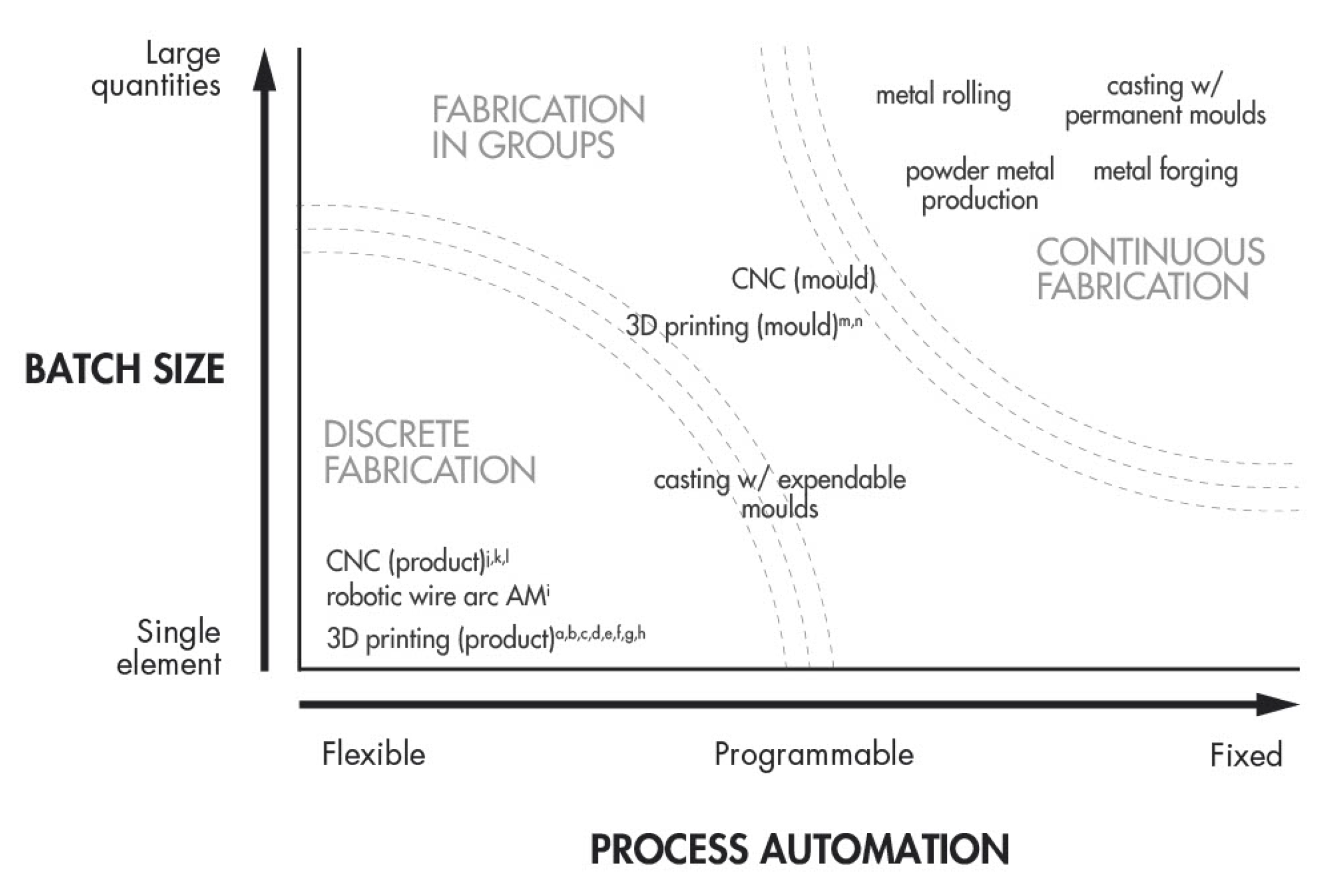
The fabrication of space-frame joints includes a wide range of manufacturing processes and tooling equipment. Joints are generally produced in batches, whose size can range from a single element to large quantities [3]. The automation of a fabrication process is defined by the frequency at which the equipment needs to be reconfigured and can be characterised as continuous, discrete or fabrication in batches [6]. Continuous processes are characterised by a fixed automation, in which the often time-expensive set-up process takes place infrequently during the production, allowing for large quantities of identical elements to be produced in-between. Examples of such processes include metal rolling, casting or powder metal production. Discrete fabrication processes on the other hand, have a flexible automation, in which the machining equipment is reconfigured before the production of each element. This category includes digital fabrication methods, where the information for the manufacturing of each joint is transferred directly from the digital design software to the manufacturing tool. Such examples include CNC-milling, robotic fabrication and 3D printing among others. Fabrication in batches describes an in-between process, in which the level of automation is programmed at frequent intervals of the fabrication process. It therefore simultaneously offers the benefits of customization and automation with the re-programming of the manufacturing process. For example, ref. [35] proposed the casting of metal joints into sand-printed moulds, while the casting process produces geometrically identical elements, the moulds have a limited lifespan, therefore enabling the reuse of their material to print a mould of a different geometry.
Figure 2 describes a classification of the different joint fabrication processes from the literature according to their batch size and level of automation [6]. Every fabrication process falls into one of these categories and can be positioned accordingly on the graph. When time- and cost-effective manufacturing of joints is considered, a fixed automation with large batch sizes is more efficient; however, it is restrictive on the variability of the generated joints. On the other hand, when the complex geometry of the design is the driver for the fabrication, flexible automation with single-element batches is most appropriate, but with potential implications for project cost. The approach developed in this paper allows a quick, comparative evaluation of the effect that different fabrication processes will have on the construction complexity of a structure and hence leads to an informed choice of the manufacturing process.

2.3. Joint Tolerance

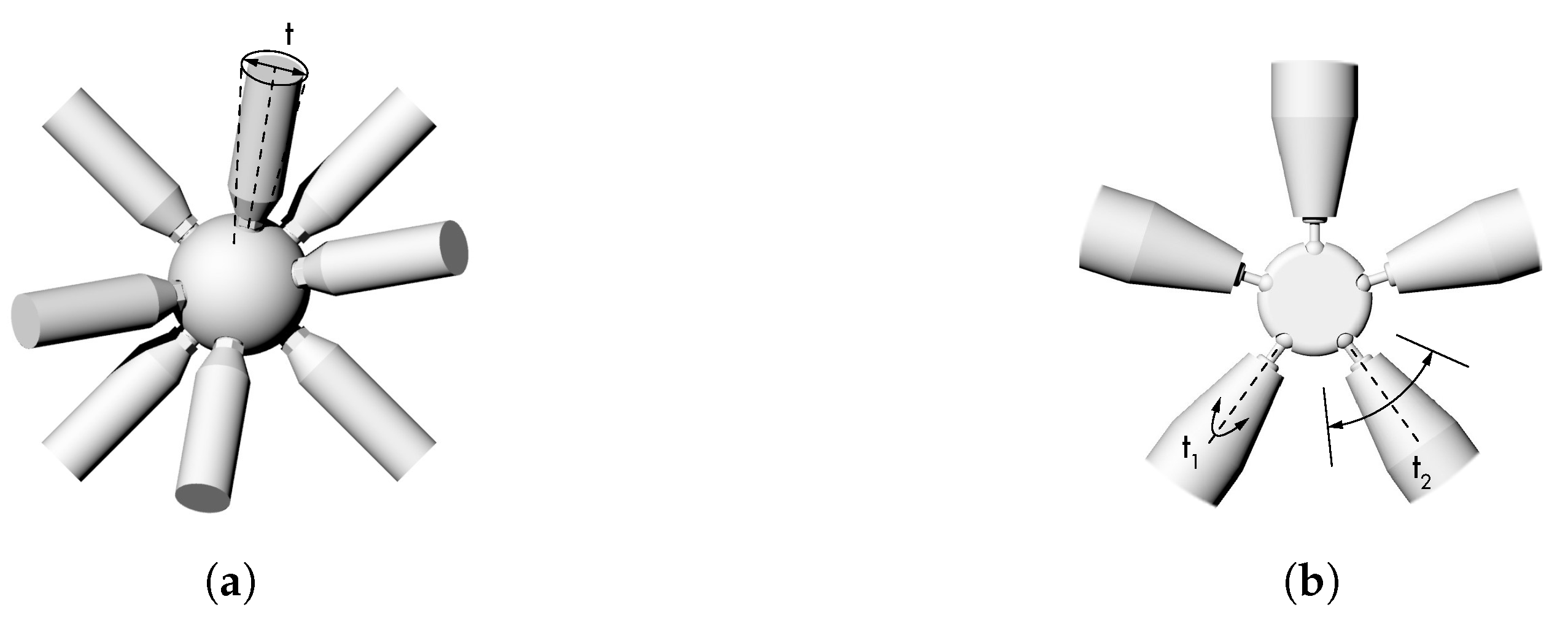
In the context of space-frame joints, tolerance can be expressed as the variability between the angles at which members meet. In terms of angle variability, every joint design has an embedded capacity to accommodate a level of tolerance in the angles at which its members meet. Depending on the specific design, this tolerance is either radial, around the member’s centroidal axis, or specific to a plane of rotation, as shown in Figure 3. When the angle difference between two joints is smaller or equal to the joint’s embedded tolerance, they can still be fabricated as members of the same batch [6]. The selection of the joint design is therefore a key factor in the fabrication process. For this paper, every joint is considered to carry an embedded tolerance, which represents the combined result of both the joint design and the construction tolerances. In practice, it describes the rotational freedom that a member has, when rotating perpendicular to its axis, while connected to a joint (Figure 3a). When a structure’s joints are clustered into fabrication batches, members of the same cluster must have an angle difference smaller than or equal to the fabrication tolerance.

3. Research Methodology

The focus of this paper is to develop a novel formulation of the k-means algorithm to efficiently cluster space-frame joints into fabrication clusters. The method developed is presented on a small-scale, two-dimensional truss case study, which offers direct insight into the angles of the structure’s joints and their cluster compactness. The analysis of joint angles presented is identical for 2D and 3D joint angles [6], rendering the method robust and fully transferable to more complex structures. The method is then applied on a freeform, large-scale space-frame structure, based on a real building, to validate its efficiency and highlight the benefits of its application in practice.
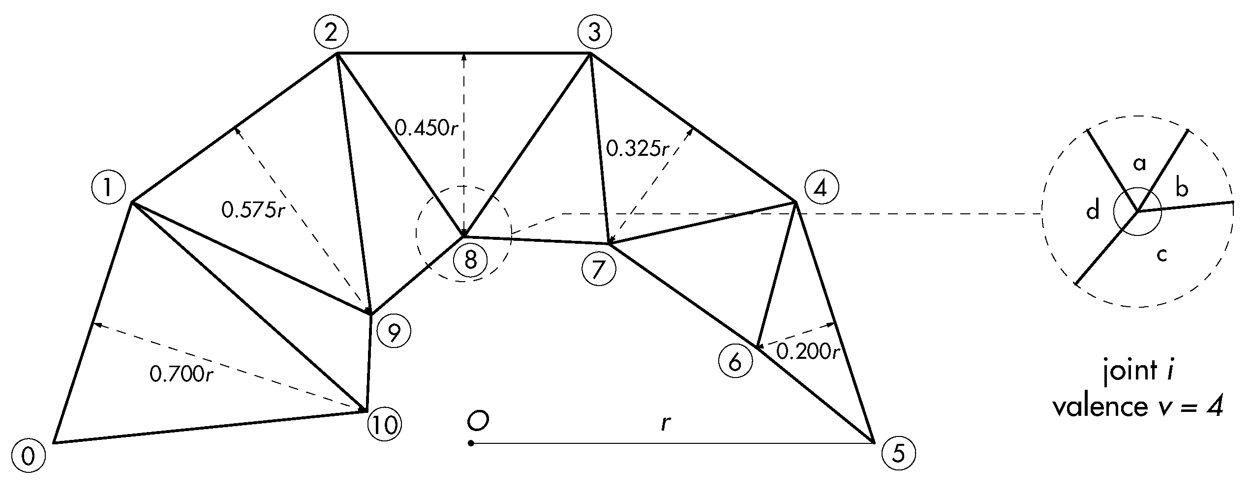
The two-dimensional truss is generated from an arc of constant curvature, with non-uniform depth, to ensure sufficient variability in the joint angles for the clustering process. An arc of r = 25 m is subdivided into five equal segments, the midpoints of which are offset normal to the arc to create the truss structure. Starting with an offset depth of 0.7r in the first bottom layer joint, the depths are consecutively decreased by a constant amount, when the bottom chord joints are taken in turn, until a depth of 0.2r is reached for the last one (Figure 4). The dataset of the joint angles generated is presented in Table 2.

3.1. Clustering Joints of Different Valence

During the clustering analysis, the difference between joint angles is calculated to assess their distance. For joints of the same valence, a simple calculation of the absolute angular distance between every pair of angles is required. This is shown in Table 3a, where joints 1 and 2 of the truss structure are compared. When the joints compared have different valences, however, further analysis is required. In practice, such joints could still have the same geometry and be fabricated in the same batch, but some of the connections would remain unused in the final structure. Therefore, no tolerance needs to be considered for the angles that represent unused connections. In the context of clustering analysis, angular distances only need to be calculated for the pair of angles, in which both joints have a connected member. Table 3b describes this scenario, when joints 1 and 6 of the case study are compared.
When both joints that are compared have a valence smaller than the maximum valence of the structure (v m a x = 4), the overall number and distribution of the empty cells can play a critical role in the clustering analysis. When there is an empty cell in a row, the specific distance is not calculated and remains empty, as described in the case of Table 3b. If there is an empty cell on every row, in either of the joints’ angles, then the final calculated distance between the two joints will be null. This would apply in the comparison of joints 0 and 5 of the case study, which both have a valence of two, when the distribution of empty cells is as shown in Table 3c. This comparison would have been driven by the relative position of the empty cells and not by the angle values and their respective distance, therefore leading to poor clustering results. It is therefore necessary to ensure that a comparison between two joints is avoided, when their angle configuration is such that there is an empty cell in each row of the matrix. A counter is thus introduced, which penalises such cases and ensures the comparison between joints is only driven by the relative distance of their angles and not the distribution of empty cells, as shown in Table 3c.

3.2. New Formulation of the k-Means Initialisation Method

The clustering analysis starts with the initialisation method, which can substantially impact the cluster compactness, depending on the criteria for the selection of the initial cluster centres—dataset density or cluster centre distribution (distance). This paper establishes a novel method to select initial cluster centres that are placed in both dense and distributed areas across the dataset.

3.2.1. Density Distribution

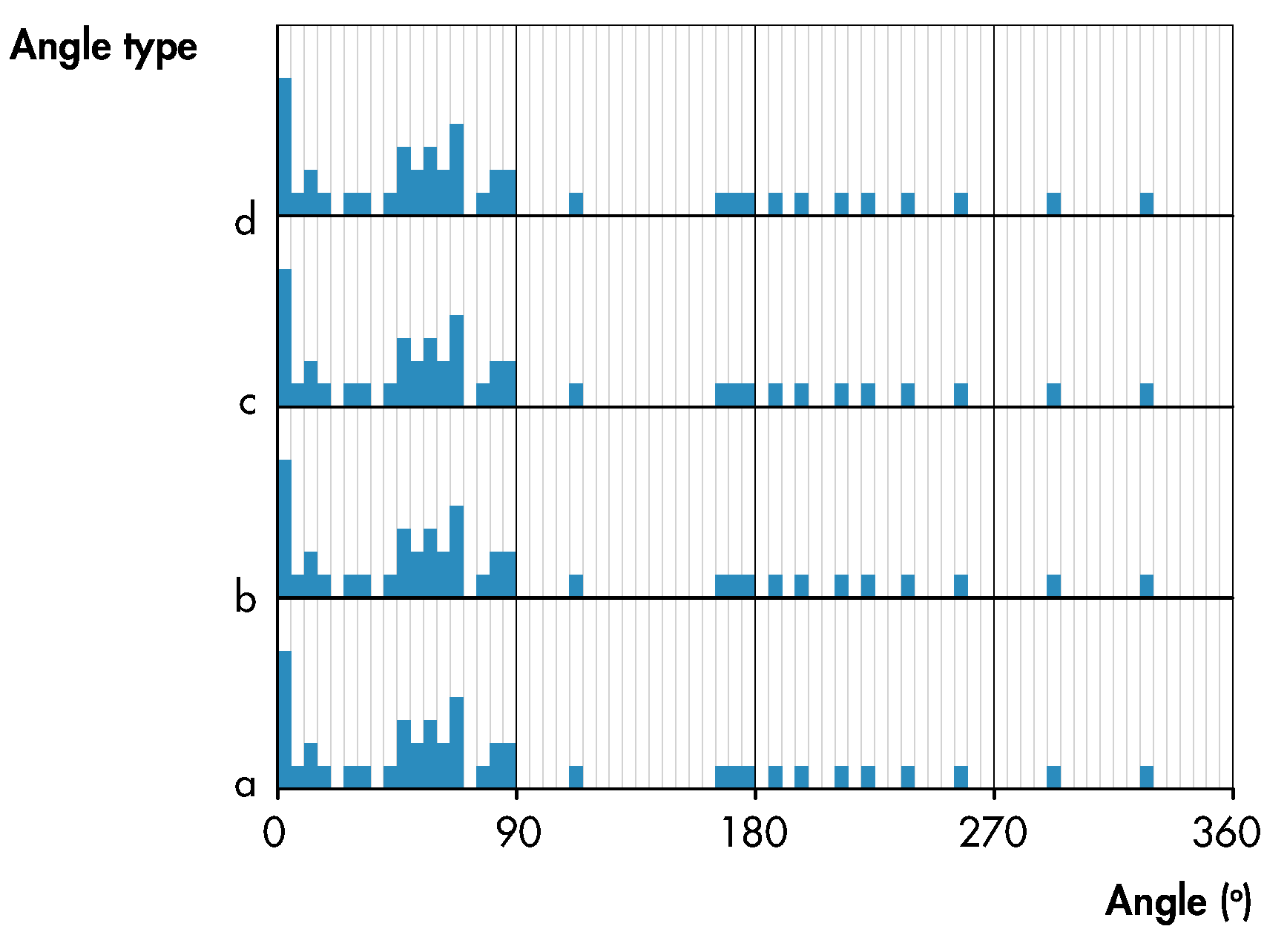
An analysis of the density distribution is carried out and a frequency histogram is plotted for each of the four angles of the case study joints (a, b, c, d), as demonstrated in Figure 5. Every row of the graph describes the frequency histogram of a different angle. The horizontal axis represents the angle values, which lie within the range of (0, 360), while the height of each frequency window is determined by the number of joints that have an angle within this range of values. The width of the frequency windows can vary, depending on the degree of detail required by the designers in each project. In the authors’ experience, the width of 5 , used in this paper, provides a compact yet detailed visualisation of the dataset.
The density distribution is carried out considering all possible configurations of the joints included in the matrix A[2vn, v], as described in Figure 1a. Since every joint is described by 2v configurations, every angle value of the same joint appears twice in every column of the dataset. This repetition of values leads to every column of the dataset containing identical values with each other, but in a different order. In effect, the frequency histograms of the different angles end up being identical as well.

3.2.2. Joint Ranking

The first cluster centre is selected based on the density distribution, while previous studies on adaptive sampling suggest a random selection of the initial cluster centre [27,28,31,49]; placing it in the densest area of the dataset has been found to enhance the efficiency of the analysis. Every joint is assigned a density ranking, r d e n s i t y , which is calculated as the sum of the value of the frequency windows, in which all their angles belong:
r d e n s i t y = j = 1 v f j ,
where f j is the value of the frequency window for the angle j of the joint and v is the maximum valence of the dataset. The first cluster centre is selected as the joint with the highest density ranking.
Once the first cluster centre has been selected, every joint is assigned a distance ranking, r d i s t a n c e , according to its Euclidean distance to (all) the previously selected cluster centres. The distance is calculated for each angle of the joint and the final ranking is the sum of all distances, as described below:
r d i s t a n c e = j = 1 v ( x j x ¯ j ) 2 ,
where x j and x ¯ j describe the angle value j of the joint and the cluster centre, respectively, and v is the maximum valence of the dataset. This ranking is dependent on the position of the formerly selected cluster centres and is therefore updated every time a new cluster centre is selected. The r d e n s i t y previously calculated, on the other hand, is dependent only on the angle values present in the dataset and thus remains constant throughout the whole process.
Following this process, every joint has two rankings, one density- and one distance-based. Due to the high diversity in the scale of their values, they are normalised to the range of [0, 1]. These rankings then form the basis for the selection of each consecutive cluster centre in the seeding process. The relative efficiency of the former over the latter is highly sensitive to the project-specific density distribution and the total number of clusters required. A weighting factor w is hence introduced to balance their effect on the initialisation process. The final ranking of a joint is therefore given by:
r = ( 1 w ) r d e n s i t y + w r d i s t a n c e
where w ∈ [0, 1] is the weighting factor used. Due to the high computational efficiency of the k-means clustering algorithm, designers can run an initial analysis for various values of w in the early stages of their design development and identify the value that yields the minimum intracluster variance for their designs.

3.2.3. Weighting Factor w

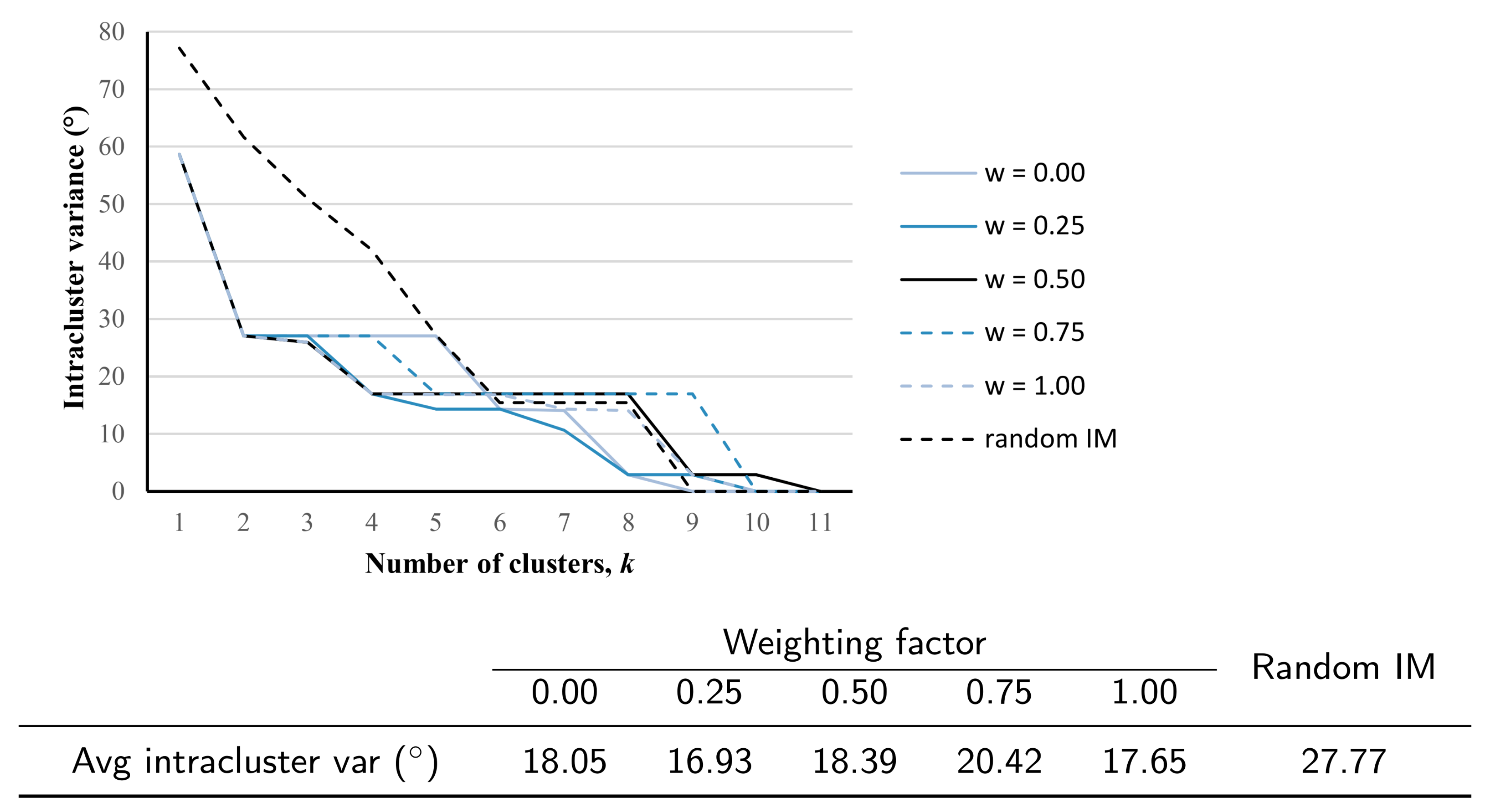
An initial analysis is run to evaluate the algorithm’s performance for different values of w and identify the one generating the clusters with the minimum intracluster variance. Given the small scale of the case study, the analysis was carried out for every possible number of clusters, k ∈ [1, 11]. The range of possible values for the weighting factor is [0, 1], with low values representing a selection of initial cluster centres in areas of high density, and high values describing a selection of initial cluster centres that are well-separated from each other. A subsection of five values of the weighting factor was evaluated for the scope of this study, w ∈ [0, 0.25, 0.50, 0.75, 1], which, in the authors’ experience provides a thorough yet efficient overview of its performance. For every weighting factor analysed, joints were clustered into all possible numbers of clusters, k∈ [1, 11]. The maximum intracluster variance of the generated clusters was then extracted, providing an overview of the factor’s performance. The initialisation method was also benchmarked against the original Lloyd’s algorithm that uses a random sampling for the initial cluster centres. The outcomes of the random initialisation were obtained by running the algorithm 25 times and selecting the overall minimum intracluster variance for comparison, as described in [30,32].
The results, shown in Figure 6, demonstrate that the proposed algorithm yields improved clustering results for most values of w, when compared to the original k-means algorithm. This is particularly evident for smaller values of k, where the intracluster variance generated with the proposed initialisation method is up to 35% lower, compared to the one generated with a random initialisation (k = 2), while this percentage gradually drops, as the number of clusters increases, certain values of the weighting factor consistently generate more effective results.
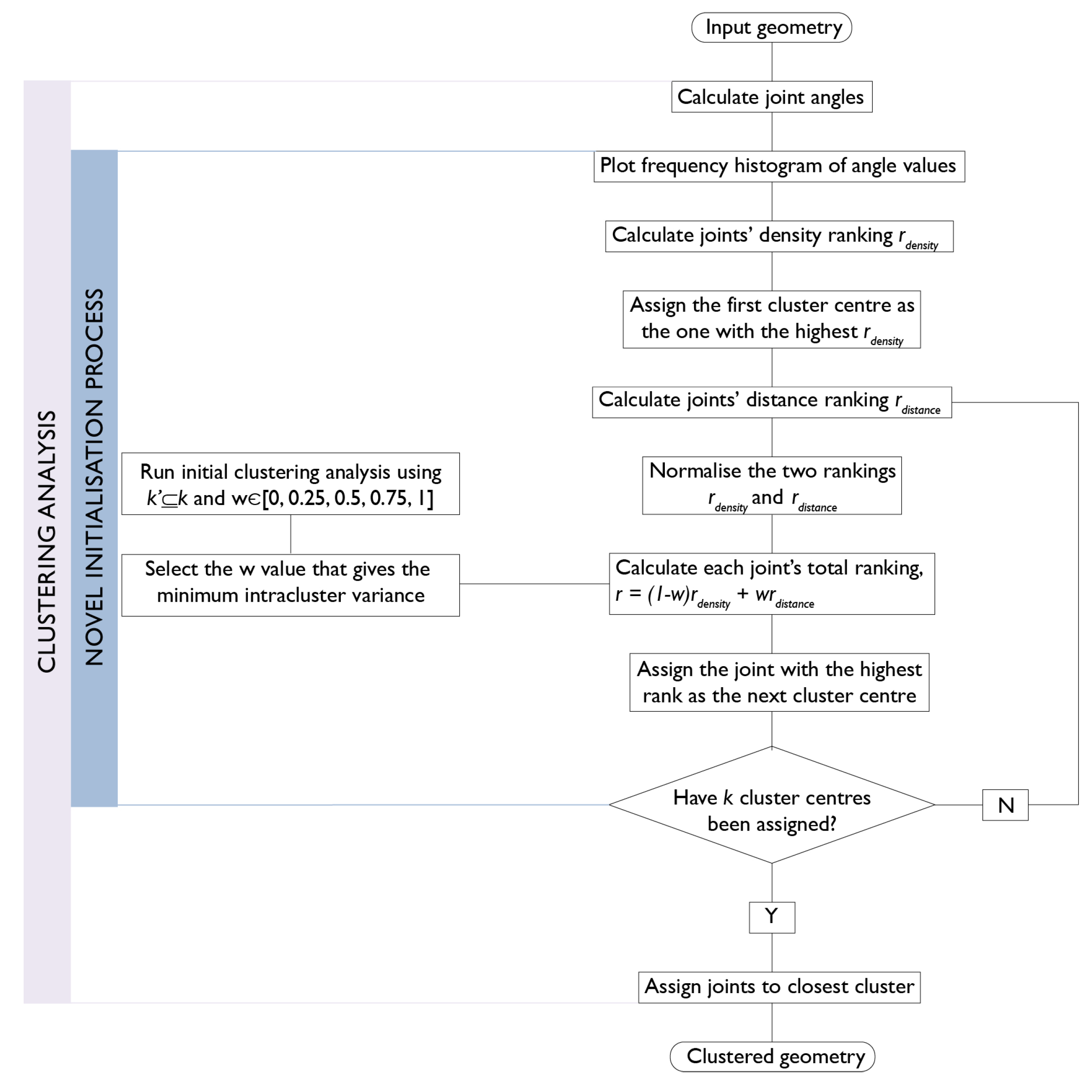
The high diversity in the resulting intracluster variance of the generated clusters, when different weighting factors are used, demonstrates the algorithm’s sensitivity to the initialisation method. The relative effectiveness of the different weighting factors changes, as joints are grouped into different numbers of clusters. This highlights that both the weighting factor and the number of clusters play an important role in achieving efficient clustering results. The overall performance of the factors studied was evaluated by calculating the average intracluster variance of the generated clusters, as shown in Figure 6. As the results show, the performance of different weighting factors is comparable and substantially better than the random initialisation. The factor w = 0.25 had the overall highest performance and was therefore used for this case study. The fact that it is closer to the value of 0 than 1 implies that, for this specific case study, selecting the initial cluster centres in dense areas of the dataset, rather than distributing them, yields improved results. Figure 7 describes the steps of the novel initialisation method developed and its integration with the other steps of the k-means clustering analysis.
The results of the clustering analysis are finally overlaid with the information regarding the joint fabrication. The two joint designs described in Figure 3 are considered. The SEO joint (Figure 3a) allows for a minimal tolerance to account for manufacturing equipment and assembly contingencies, which is assumed to be 2 . The HUBS joint (Figure 3b), on the other hand, allows for a planar tolerance of up to 30 . When overlaying this information on the graph, it becomes evident that the selection of the joint design will greatly impact on the overall fabrication process. Figure 8 describes the joint fabrication of the truss structure analysed, if low or high tolerance joints are selected. Such information can meaningfully drive the fabrication and design development of a project, depending on available resources, time and cost.

4. Real-Building Case Study

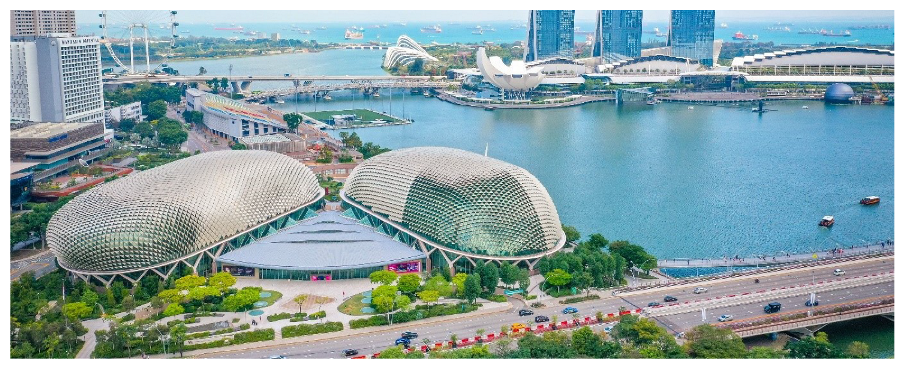
The analysis method developed was applied on a large-scale, complex structure to highlight its benefits in practice. The envelope of the Singapore Arts Centre was used as a realistic case study for the application of the proposed methodology. The building comprises two structures, the Concert Hall and the Lyric Theatre, both of which have freeform roof structures, as shown in Figure 9. The geometry of the Lyric Theatre was recreated, according to the information provided in [1]. The generated digital model of the space-frame roof has a constant structural depth of 0.9 m and contains 3300 joints. The goal of the analysis was to evaluate the construction complexity of the generated geometry and explore alternative fabrication scenarios. Since the geometry was recreated to represent an existing building, this study validates the applicability of the proposed workflow in practice, where it can inform the selection of appropriate joint design and fabrication methods in early stages of the design development.

4.1. Description

The first step of the proposed methodology requires the number of clusters k as an input, and a selection of the weighting factor w. Assuming that this analysis is realised during the early stages of design development, and that these parameters have not been defined by the brief, the roof structure is analysed for multiple values of k ∈ (10, 50, 100, 200), to obtain an overall estimation of the cluster characteristics. The joints are clustered for each value of k, using different values of the weighting factor w∈ [0, 0.25, 0.50, 0.75, 1.00]. The factor that generates the most compact clusters will then be taken forward for the detailed design of the fabrication process.

4.2. Results

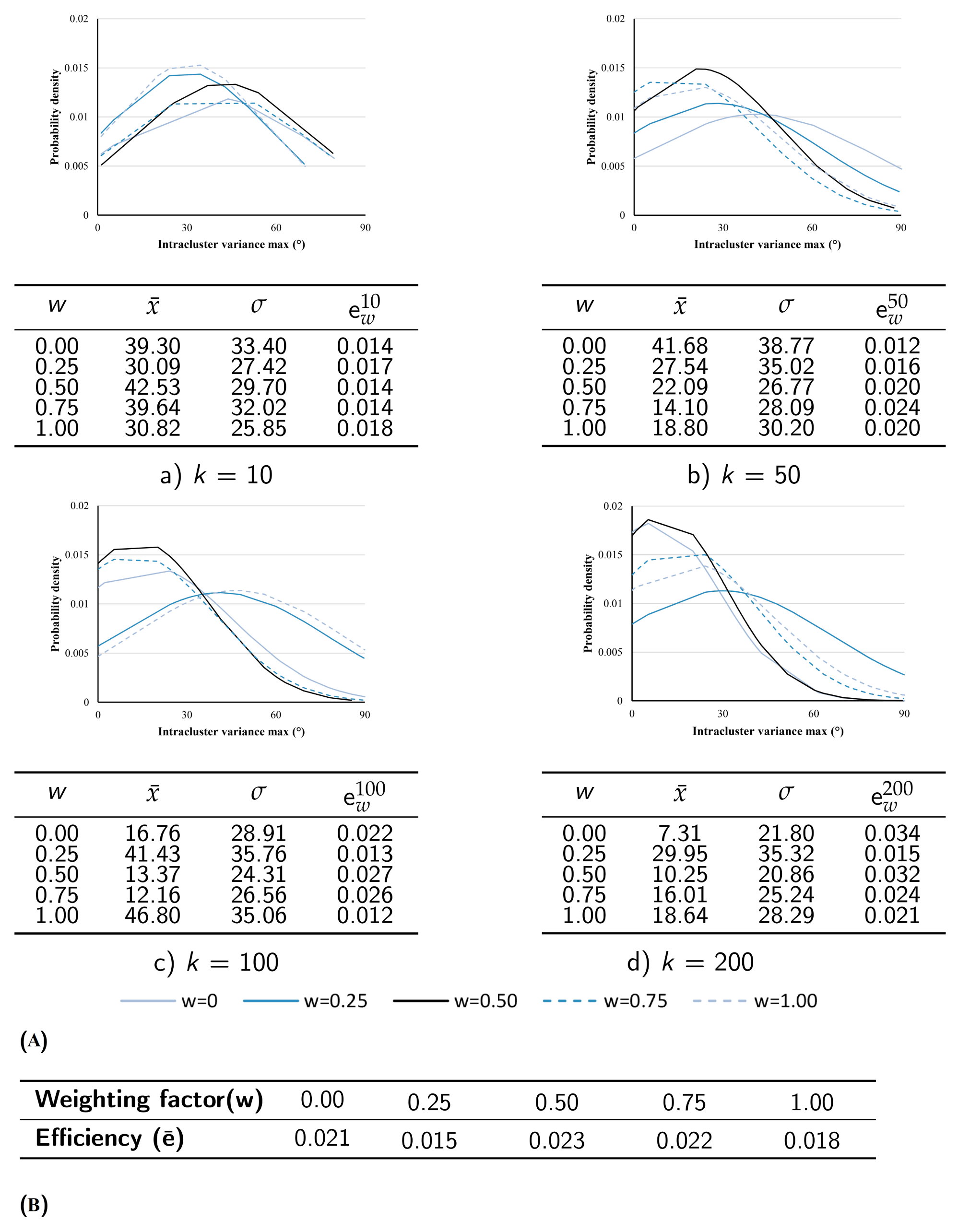
Due to the large-scale structure, the characteristics between different clusters are highly diverse. As a result, a simple extraction of the maximum intracluster variance for a given set of k and w values would not capture the variance distribution and the properties of different clusters, as in the previous example (Figure 6). The standard normal distribution of the maximum intracluster variance is therefore plotted for all cluster values, when different weighting factors are applied, as shown in Figure 10A. The horizontal axis describes the intracluster variance and the vertical axis the probability density of this variance for the respective k and w values. An efficient clustering analysis would exhibit a high probability density for low values of intracluster variance, and would therefore have a low mean and a low standard deviation. The efficiency of a weighting factor e w k , when joints are grouped into k clusters, is evaluated as the inverse of the sum of the mean and standard deviation for a given value of k, as described below:
e w k = 1 x ¯ w k + σ w k
where e is the efficiency ranking of the weighting factor w, x ¯ is the mean and σ the standard deviation for the w and k values given. The overall efficiency of each weighting factor is calculated as the average of its efficiency ranking for the different values of k studied. Figure 10 presents the average efficiency of the weighting factors evaluated. w = 0.5 has the highest overall performance across all values of k and is therefore used for this study.
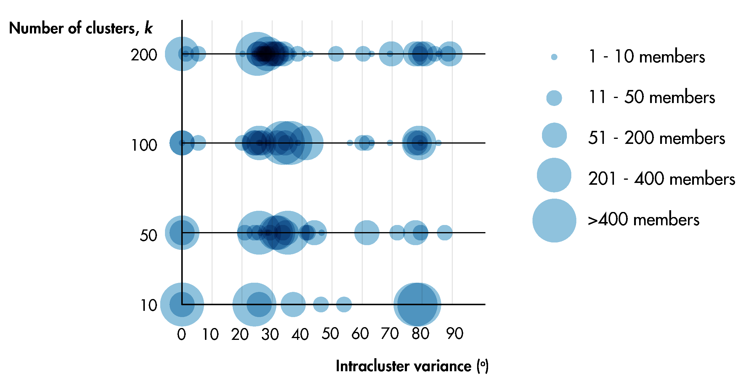
Figure 11 summarizes the relationship between the sizes, number of clusters and the respective intracluster variance to extract further details. Each horizontal line corresponds to a different value of k and each circle represents a cluster. The size of the circle is indicative of the number of joints in that cluster and its position on the x-axis represents the intracluster variance of the respective cluster. Hence the further left on the x-axis a circle is, the more compact that cluster. An efficient clustering algorithm would lead to a gradual shift in all the circles towards the left side of the graph, as the number of clusters increases, which would signify clusters of higher homogeneity between their members.
Observing the results of the clustering analysis in Figure 11, the size of clusters decreases as the value of k rises, indicating that a higher number of smaller clusters is created. Simultaneously, the large clusters of high intracluster variance, which can be observed for k = 10 (intracluster variance > 70 ) are gradually split into smaller, more compact clusters, represented by the smaller-sized circles at lower values of intracluster variance in the k = 50, 100, 200 rows. Moreover, the clusters, whose intracluster variance lies between 15 and 55 , gradually obtain higher compactness, as k rises. These observations highlight the efficiency of the algorithm in generating compact clusters as k increases. This relationship between the number of clusters and the intracluster variance plays an important role in designing an efficient fabrication process, as it describes the number of clusters that have similar characteristics. Figure 12 presents a frequency histogram describing this relationship for different values of k. The high number of clusters that have a minimal intracluster variance of only a few degrees is particularly interesting, as these are clusters of practically identical items. From a fabrication perspective, this means that their fabrication time and cost would be minimal, as their items would have similar geometry and could be produced with continuous processes. For k = 50 there are 24 such clusters, for k = 100 there are 69 clusters and for k = 200 there are 148. The increase in number of clusters of identical items is hence not proportional to the number of clusters; the higher the value of k, the higher the percentage of clusters of practically identical items required.

4.3. Assessing Fabrication Complexity

Comparative studies for different fabrication processes and joint designs can guide designers in selecting the most efficient fabrication method and joint designs for their structures. In terms of the fabrication process, the batch size and level of automation required will define whether a discrete or continuous process is more effective. In terms of the joint design, on the other hand, joints with a high embedded tolerance can accommodate significant intracluster variance, while joints with a small tolerance are more efficient in compact clusters. Due to the high impact that the fabrication automation and joint design tolerance have, their appropriateness can significantly vary, depending on the value of k.
If joints are grouped in a small number of clusters (k = 10), the large size of the generated clusters suggests that a continuous fabrication process, favouring the mass-production of identical elements, would be more efficient. However, due to the great variability in the members of each cluster, the joint design would need to accommodate a high level of tolerance. Therefore a joint design similar to the one described in Figure 3b, would be better suited, as demonstrated in Table 4, Scenario 1.
As k increases, the characteristics of the different clusters vary significantly. For this case study, the results for k = 200 are analysed in more detail. As previously described, there is a high number of large clusters of near-identical elements, while at the same time there is a small number of clusters with a high intracluster variance. If a joint type of minimal tolerance is selected (Figure 3a), then a combination of both discrete and continuous fabrication would be most efficient. The 148 clusters of near-identical items could be fabricated with a continuous process, while discrete fabrication could incorporate the variability of the remaining 52 clusters, as shown in Table 4, Scenario 2. On the other hand, if a joint with a high level of tolerance is selected, then a continuous process could be applied to all elements. The fabrication process could enable the production of large batches of identical members, in the case of the 148 clusters of minimal intracluster variance, while the joint design would also accommodate the variance of the remaining clusters (Table 4, Scenario 3). Finally, if two different joint types could be used, a joint that allows for minimal tolerance could be applied for the clusters of no intracluster variance (148 clusters) and a joint design that can accommodate variability for the remaining clusters (52 clusters), as described in Table 4, Scenario 4.
The analysis presented highlights that, when small values of k are used, all clusters share similar characteristics and the selection of the fabrication method and joint design is a linear process. As k increases, evaluating the fabrication complexity becomes a highly complex process in itself, as cluster sizes and variability are scattered. The co-existence of both large and small clusters suggests that a combination of different fabrication processes would be the most appropriate, with a continuous process for large clusters and a discrete process for the small clusters. In addition, the significant diversity in the level of intracluster variance implies that different levels of embedded variability in the joint design would be beneficial; applying multiple joint designs would therefore contribute to further facilitating fabrication. It is thus evident that high diversity in the cluster sizes and degrees of intracluster variance render the selection of a fabrication process and joint design a challenge. The computational workflow developed facilitates this process, by enabling the assessment of different fabrication options in early stages of the design.

5. Discussion

A novel initialisation method for the k-means algorithm has been developed, that selects the initial cluster centres according to the density distribution of the joint angles and the distance between them. Existing research has proposed deterministic approaches, in which the impact of the dataset density or the distance between initial cluster centres remains constant during the seeding process, whenever the algorithm is applied to different datasets [27,28,29,30,31,32]. The initialisation method developed, however, introduces a weighting factor that calibrates the relative impact of the density and cluster centres’ distance on the seeding process. Informed by the geometrical characteristics of the specific structure analysed, the value of the weighting factor is automatically adjusted to ensure improved clustering results. The performance of the initialisation method has been compared against the random initialisation of the original k-means algorithm [15], and shows to be 35% more efficient.
The case study analysed demonstrated that the design of an efficient fabrication process is highly complex, due to the variety of manufacturing methods available and the diverse characteristics that joint clusters present, while this might be expected in a building of such scale and geometrical complexity, the analysis presented enables a critical assessment of different fabrication and construction options. The results demonstrate that continuous fabrication processes and joint designs accommodating high levels of tolerance can be more appropriate for achieving an efficient construction process. However these findings are only valid when a reduction in the construction complexity is the main driver in the decision-making process. If the criteria change, the interpretation of the clustering analysis would need to adapt accordingly. For example, if achieving a specific geometry is the driver, a discrete fabrication process, which generates bespoke elements, would be appropriate. In addition, the availability of the different fabrication processes also plays a critical role. It therefore becomes evident that project-specific requirements and limitations are the drivers for the interpretation of the clustering analysis results and the design of an efficient fabrication process. The workflow developed provides a robust and automated tool for the analysis and consideration of such parameters in the early stages of design development.
This observation triggers a discussion of the relation between customisation and the performance of contemporary computational tools. On the one hand, the k-means algorithm is a widely used clustering algorithm, applicable in diverse contexts. Nevertheless, the randomness embedded in its seeding process can substantially compromise its performance, depending on the properties of the dataset [19]. On the other hand, the proposed clustering algorithm is a highly customised tool that responds to context-specific requirements. This is further accentuated by the introduction of the weighting factor, whose value is informed by the geometry of the given structure analysed. There is hence a clear distinction between heuristic algorithms that are applicable in diverse contexts, such as the k-means, and highly customised tools. Heuristic algorithms are efficient procedures that can find high-performing solutions, even if they are not optimal, in a quick and computationally efficient manner [51]. Their speed of execution and flexibility in formulation enable their application in diverse sets, that are often difficult to model. The method proposed, on the other hand, is an adaptation of the k-means that outperforms the heuristic algorithm. However, it has been developed in the context of space-frame joints and therefore remains applicable to this specific type of problem. Hence, it is essential to understand the limitations of the tools applied to solve a given design problem and to recognise the project-specific parameters that can affect their performance.

6. Conclusions

This paper proposes a novel framework for the evaluation of the construction complexity of freeform space-frame structures, as a factor of geometrical variability in their joints. It has been shown that designing an efficient construction process is highly complex, both due to the variety of available manufacturing tools and processes, as well as the high diversity in the distribution of geometrical variability within a single structure. A new initialisation method has been developed to cluster joints into fabrication batches, generating substantially more compact clusters compared to existing methods. This has been integrated into a computationally efficient and automated process that allows a detailed overview of alternative construction scenarios, in which different combinations of fabrication processes are assessed. It is thus possible to identify the most efficient solution, according to project-specific requirements and constraints, while applicable at any stage of the project development, the proposed method is most useful when applied in early stages of the design, when it can drive the project development in an informed manner. The robustness of the method makes it applicable on diverse projects in practice, where it can provide a framework for the critical evaluation and informed application of novel and existing fabrication processes and reduce the construction complexity of large-scale, freeform space-frame structures.

Author Contributions

Conceptualization, A.K., P.S. and M.E.; methodology, A.K., P.S. and M.E.; software, A.K.; validation, A.K., P.S. and M.E.; formal analysis, A.K., P.S. and M.E.; investigation, A.K.; resources, P.S.; data curation, A.K.; writing—original draft preparation, A.K.; writing—review and editing, A.K., P.S. and M.E.; visualization, A.K.; supervision, P.S. and M.E.; project administration, P.S.; funding acquisition, P.S. All authors have read and agreed to the published version of the manuscript.

Funding

This study was supported by the EPSRC Centre for Decarbonisation of the Built Environment (dCarb) [Grant Ref: EP/L016869/1].

Data Availability Statement

The data presented in this study are available on request from the corresponding author.

Acknowledgments

The authors would like to express their gratitude to LANIK Engineers and in particular to Goni Josu and Alain Cabanas for their views and insights into the opportunities and challenges of the construction of space-frame structures in practice.

Conflicts of Interest

The authors declare no conflict of interest. The funders had no role in the design of the study; in the collection, analyses, or interpretation of data; in the writing of the manuscript; or in the decision to publish the results.

References

  1. Klimke, H.; Sanchez, J.; Vasiliu, M.; Stühler, W.; Kaspar, C. The Envelopes of the Arts Centre in Singapore. In Proceedings of the IABSE Symposium: Towards a Better Built Environment—Innovation, Sustainability, Information Technology, Melbourne, Australia, 11–13 September 2002. [Google Scholar] [CrossRef]
  2. Sanchez-Alvarez, J. Practical aspects determining the modelling of the space structure for the free-form envelope enclosing Baku’s Heydar Aliyev Cultural Centre. In Proceedings of the Symposium of the International Association for Shell and Spatial Structures (50th. 2009. Valencia), Evolution and Trends in Design, Analysis and Construction of Shell and Spatial Structures: Proceedings, Valencia, Spain, 28 September–2 October 2009. [Google Scholar]
  3. Kalpakjian, S.; Schmid, S. Manufacturing Engineering and Technology, 7th ed.; Pearson: New York, NY, USA, 2013. [Google Scholar]
  4. Lan, T.T. Space Frame Structures. In Structural Engineering Handbook; Wai-Fah, C., Ed.; Number 1999; CRC Press: Boca Raton, FL, USA, 2005; pp. 1–50. [Google Scholar] [CrossRef]
  5. Koronaki, A.; Shepherd, P.; Evernden, M. Geometry optimization of space frame structures for joint modularity. In Proceedings of the Creativity in Structural Design, Boston, MA, USA, 16–20 July 2018. [Google Scholar]
  6. Koronaki, A.; Shepherd, P.; Evernden, M. Rationalization of freeform space-frame structures: Reducing variability in the joints. Int. J. Archit. Comput. 2020, 18, 84–99. [Google Scholar] [CrossRef]
  7. Asadpoure, A.; Guest, J.K.; Valdevit, L. Incorporating fabrication cost into topology optimization of discrete structures and lattices. Struct. Multidiscip. Optim. 2015, 51, 385–396. [Google Scholar] [CrossRef]
  8. Paulson, B. Designing to reduce construction cost. J. Constr. Div. 1976, 102, 587–592. [Google Scholar] [CrossRef]
  9. Ranalli, F.; Flager, F.; Fischer, M. A Ground Structure Method to Minimize the Total Installed Cost of Steel Frame Structures. World Acad. Sci. Eng. Technol. Int. J. Civ. Environ. Eng. 2018, 12, 115–123. [Google Scholar]
  10. Batta, M. Machine Learning Algorithms—A Review. Int. J. Sci. Res. 2020, 9, 381–386. [Google Scholar] [CrossRef]
  11. Carleo, G.; Cirac, I.; Cranmer, K.; Daudet, L.; Schuld, M.; Tishby, N.; Vogt-Maranto, L.; Zdeborová, L. Machine learning and the physical sciences. Rev. Mod. Phys. 2019, 91, 45002. [Google Scholar] [CrossRef] [Green Version]
  12. Wierzchoń, S.T.; Kłopotek, M.A. Modern Algorithms of Cluster Analysis; Springer: Cham, Switzerland, 2018. [Google Scholar] [CrossRef]
  13. Celebi, M.E. Partitional Clustering Algorithms; Springer International Publishing: Cham, Switzerland, 2015; pp. 1–415. [Google Scholar] [CrossRef]
  14. Xu, D.; Tian, Y. A Comprehensive Survey of Clustering Algorithms. Ann. Data Sci. 2015, 2, 165–193. [Google Scholar] [CrossRef] [Green Version]
  15. Lloyd, S.P. Least squares quantization in PCM. IEEE Trans. Inf. Theory 1982, 28, 129–137. [Google Scholar] [CrossRef] [Green Version]
  16. Ghazal, T.M.; Hussain, M.Z.; Said, R.A.; Nadeem, A.; Hasan, M.K.; Ahmad, M.; Khan, M.A.; Naseem, M.T. Performances of k-means clustering algorithm with different distance metrics. Intell. Autom. Soft Comput. 2021, 30, 735–742. [Google Scholar] [CrossRef]
  17. Jain, A.K. Data clustering: 50 years beyond K-means. Pattern Recognit. Lett. 2010, 31, 651–666. [Google Scholar] [CrossRef]
  18. Jiang, F.; Liu, G.; Du, J.; Sui, Y. Initialization of K-modes clustering using outlier detection techniques. Inf. Sci. 2016, 332, 167–183. [Google Scholar] [CrossRef]
  19. Celebi, M.E.; Kingravi, H.A.; Vela, P.A. A comparative study of efficient initialization methods for the k-means clustering algorithm. Expert Syst. Appl. 2013, 40, 200–210. [Google Scholar] [CrossRef] [Green Version]
  20. Blömer, J.; Lammersen, C.; Schmidt, M.; Sohler, C. Theoretical analysis of the k-means algorithm—A survey. In Algorithm Engineering; Lecture Notes in Computer Science—LNCS; Springer: Cham, Switzerland, 2016; Volume 9220, pp. 81–116. [Google Scholar] [CrossRef] [Green Version]
  21. Hussain, S.F.; Haris, M. A k-means based co-clustering (kCC) algorithm for sparse, high dimensional data. Expert Syst. Appl. 2019, 118, 20–34. [Google Scholar] [CrossRef]
  22. Ayech, M.W.; Ziou, D. Segmentation of Terahertz imaging using k-means clustering based on ranked set sampling. Expert Syst. Appl. 2015, 42, 2959–2974. [Google Scholar] [CrossRef]
  23. Mac Queen, J. Some methods for classification and analysis of multivariate observations. In Proceedings of the 5th Berkeley Symposium on Mathematical Statistics and Probability, Berkeley, CA, USA, 21 June–18 July 1965; University of California Press: Berkeley, CA, USA, 1967; Volume 1, pp. 281–297. [Google Scholar]
  24. Forgy, E. Cluster analysis of multivariate data: Efficiency versus interpretability of classifications. Biometrics 1965, 21, 768–769. [Google Scholar]
  25. Li, Z.; Berger, V.W. Adaptive Sampling. In Encyclopedia of Statistics in Behavioral Science; Everitt, B.S., Howell, D.C., Eds.; John Wiley & Sons, Ltd.: Chichester, UK, 2005; Volume 1, pp. 13–16. [Google Scholar]
  26. Aggarwal, A.; Deshpande, A.; Kannan, R. Adaptive sampling for k-means clustering. In Proceedings of the 12th International Workshop, APPROX 2009, and 13th International Workshop, RANDOM 2009, Berkeley, CA, USA, 21–23 August 2009; Volume 5687, pp. 15–28. [Google Scholar] [CrossRef]
  27. Katsavounidis, I.; Kuo, C.C.; Zhang, Z. A New Initialization Technique for Generalized Lloyd Iteration. IEEE Signal Process. Lett. 1994, 1, 144–146. [Google Scholar] [CrossRef]
  28. Arthur, D.; Vassilvitskii, S. k-means++: The advantages of careful seeding. In Proceedings of the SODA’07: Proceedings of the Eighteenth Annual ACM-SIAM Symposium on Discrete Algorithms, Society for Industrial and Applied Mathematics. Philadelphia, PA, USA, 7–9 January 2007; pp. 1027–1035. [Google Scholar]
  29. Khan, S.S.; Ahmad, A. Cluster center initialization algorithm for K-modes clustering. Expert Syst. Appl. 2013, 40, 7444–7456. [Google Scholar] [CrossRef] [Green Version]
  30. Gourgaris, P.; Makris, C. A Density Based k-Means Initialization Scheme. In Proceedings of the EANN ’15: 16th International Conference on Engineering Applications of Neural Networks (INNs), Rhodes Island, Greece, 25–28 September 2015; pp. 1–9. [Google Scholar] [CrossRef]
  31. El Alaoui, M.; Ben-azza, H. New initialization for clustering algorithms combining distance and density. In Proceedings of the BDCA 2017: 2nd International Conference on Big Data, Cloud and Applications, Tetouan, Morocco, 29–30 March 2017; pp. 1–5. [Google Scholar] [CrossRef]
  32. Kumar, K.M.; Reddy, A.R.M. An efficient k-means clustering filtering algorithm using density based initial cluster centers. Inf. Sci. 2017, 418–419, 286–301. [Google Scholar] [CrossRef]
  33. Yang, W.; Long, H.; Ma, L.; Sun, H. Research on clustering method based on weighted distance density and k-means. Procedia Comput. Sci. 2020, 166, 507–511. [Google Scholar] [CrossRef]
  34. Oti, E.U.; Unyeagu, S.I.; Nwankwo, C.H.; Alvan, W.K.; Osuji, G.A. New K-means clustering methods that minimize the total intra-cluster variance. Afr. J. Math. Stat. Stud. 2020, 3, 42–54. [Google Scholar]
  35. Niehe, P. Sand Printing Makes Complex Casted Structural Parts Affordable; European Press Office: Amsterdam, The Netherlands, 2017; Available online: https://www.arup.com/news-and-events/sand-printing-makes-complex-casted-structural-parts-affordable/ (accessed on 20 September 2022).
  36. Hubs. Geodesic Domes Made Simple. 2017. Available online: https://buildwithhubs.co.uk/ (accessed on 20 September 2022).
  37. Chun, J.; Lee, J.; Park, D. Topo-joint: Topology Optimization Framework for 3D-Printed Building Joints. In Proceedings of the 23rd International Conference of the Association for Computer-Aided Architectural Design Research in Asia (CAADRIA): Learning, Adapting and Prototyping, Beijing, China, 17–19 May 2018; Volume 1, pp. 205–214. [Google Scholar]
  38. Dritsas, S.; Chen, L.; Sass, L. Small 3D printers/large scale artifacts: Computation for Automated Spatial Lattice Design-to-Fabrication with Low Cost Linear Elements and 3D-Printed Nodes. In Proceedings of the CAADRIA 2017—22nd International Conference on Computer-Aided Architectural Design Research in Asia: Protocols, Flows and Glitches, Hong Kong, China, 5–8 April 2017; pp. 821–830. [Google Scholar]
  39. Sousa, J.P.; Varela, P.d.A.; Carvalho, J.; Santos, R.; Oliveira, M. Mass-customization of Joints for Non-Standard Structures through Additive Manufacturing: The Trefoil and the TriArch projects. In Proceedings of the eCAADe36: Applications in Construction & Optimization, Lodz, Poland, 19–21 September 2018; Volume 1, pp. 197–204. [Google Scholar]
  40. Tanadini, D.; Ohlbrock, P.O.; Kladeftira, M.; Leschok, M.; Skevaki, E.; Dillenburger, B.; D’Acunto, P. Exploring the potential of equilibrium-based methods in additive manufacturing: The Digital Bambloo pavilioin. In Proceedings of the IASS 2022 Symposium Affiliated with APCS 2022 Conference—Innovation-Sustainability-Legacy, Beijing, China, 19–22 September 2022. [Google Scholar]
  41. Kladeftira, M.; Leschok, M.; Skevaki, E.; Dillenburger, B. Redefining Polyhedral Space Through 3D Printing. In Proceedings of the AAG Advances in Architectural Geometry, Online, 26–29 April 2021. [Google Scholar]
  42. Kladeftira, M.; Leschok, M.; Skevaki, E.; Tanadini, D.; Ohlbrock, P.O.; D’Acunto, P.; Dillenburger, B. Digital Bamboo: A study on bamboo, 3D printed joints, and digitally fabricated building components for ultralight structures. In Proceedings of the ACADIA 2022: Hybrids & Haecceities, Philadelphia, PA, USA, 27–29 October 2022. [Google Scholar]
  43. Bach, P.; Giacomini, I.; Kladeftira, M. Self-interlocking 3D Printed Joints for Modular Assembly of Space Frame Structures. In Proceedings of the 8th Design Modelling Symposium (DMS 2022): Towards Radical Regeneration, Berlin, Germany, 26–28 September 2022. [Google Scholar]
  44. Ariza, I.; Mirjan, A.; Gandia, A.; Casas, G.; Cros, S.; Gramazio, F.; Kohler, M. In place detailing: Combining 3D printing and robotic assembly. In Proceedings of the ACADIA, Mexico City, Mexico, 18–20 October 2018; pp. 312–321. [Google Scholar] [CrossRef]
  45. LANIK. Lanik Ingenieros | Hacemos su Proyecto Realidad. 2018. Available online: http://www.lanik.com/ (accessed on 8 September 2022).
  46. MERO. Home—MERO. 2018. Available online: https://www.mero.de/ (accessed on 8 September 2022).
  47. Octatube. Octatube | Realizing Challenging Architecture. 2018. Available online: https://www.octatube.nl/ (accessed on 8 September 2022).
  48. Aghaei Meibodi, M.; Giesecke, R.; Dillenburger, B. 3D Printing sand mold for casting bespoke-Digital Metal: Additive Manufacturing for Casting Metal Parts in Architecture. In Proceedings of the Intelligent and Informed—Proceedings of the 24th International Conference on Computer-Aided Architectural Design Research in Asia, CAADRIA, Wellington, New Zealand, 15–18 April 2019; Volume 1, pp. 133–142. [Google Scholar]
  49. Bhattacharya, A.; Eube, J.; Röglin, H.; Schmidt, M. Noisy, Greedy and Not So Greedy k-means++. In Proceedings of the 28th Annual European Symposium on Algorithms, ESA 2020, Pisa, Italy, 7–9 September 2020; Volume 1, pp. 1–21. [Google Scholar]
  50. Dagli, M. Singapore Arts Centre, Singapore. 2019. Available online: https://unsplash.com/photos/Uii70ORiFPE (accessed on 26 May 2020).
  51. Martí, R. Exact and Heuristic Methods in Combinatorial Optimization; Springer: Berlin/Heidelberg, Germany, 2022. [Google Scholar]
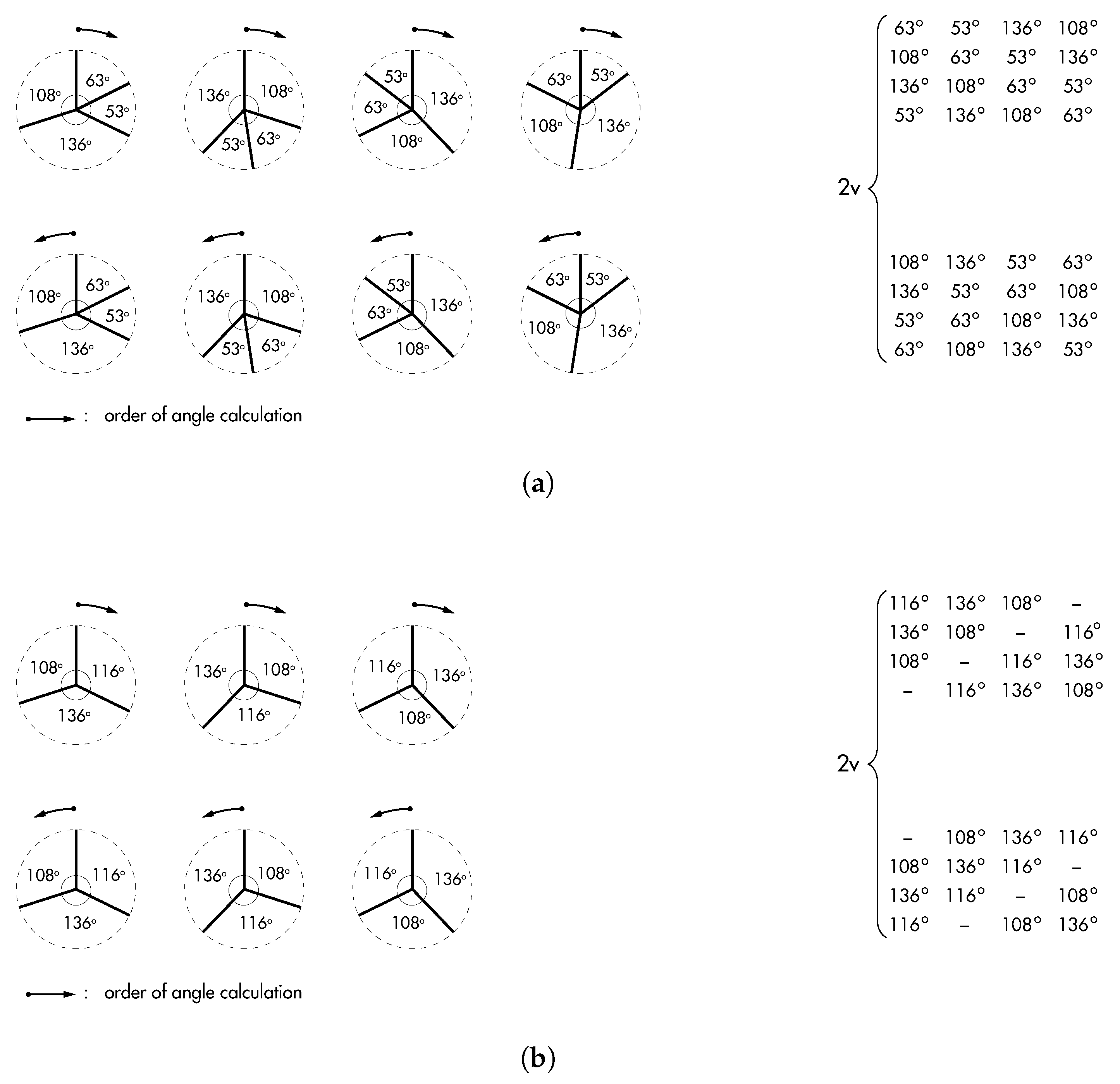
Figure 1. Every joint can be described by 2v possible configurations of its angles, where v is the maximum valence in the structure studied. Each of these configurations are stored in a matrix A with 2vn rows and n columns, where v is the maximum valence and n is the number of joints in the structure. In the case of joints of a smaller valence, the left over cells remain empty. (a) The 2v = 8 possible angle configurations for a joint with a valence v = 4. (b) The 2v = 8 possible angle configurations for a joint with a valence v = 3, when placed in a structure of a maximum valence of v = 4.
Buildings 13 00962 g001
Figure 2. Classification of joint fabrication processes depending on batch size and process automation, and literature examples for each (adapted form [6]). The boundaries between different fabrication types remain fluid and cannot be strictly defined. (a) Hubs [36], (b) Chun et al. 2018 [37], (c) Dritsas et al. 2017 [38], (d) Souza et al., 2018 [39], (e) Tanadini et al., 2022 [40], (f) Kladeftira et al. 2021 [41], (g) Kladeftira et al., 2022 [42], (h) Bach et al., 2023 [43], (i) Ariza et al. 2018 [44], (j) LANIK Engineers [45], (k) MERO [46], (l) Octatube [47], (m) Niehe 2017 [35], (n) Aghaei Meibodi et al., 2019 [48].
Buildings 13 00962 g002
Figure 3. The tolerance embedded in different joint designs. (a) Joint design with minimal tolerance [45,46]. The tolerance is measured rotationally around the members’ axis. (b) Joint design with a high level of tolerance [36]. The level of tolerance differs, depending on the plane the members move in. Reprinted with permission from [6].
Buildings 13 00962 g003
Figure 4. A two-dimensional truss with geometrically varying joints.
Buildings 13 00962 g004
Figure 5. Frequency histogram of the density distribution of the structure’s joint angles.
Buildings 13 00962 g005
Figure 6. Comparison of the novel initialisation method to the random initialisation of the k-means algorithm. The average intracluster variance of the generated clusters for the different weighting factors shows that the novel method outperforms the random initialisation of k-means.
Buildings 13 00962 g006
Figure 7. The pseudocode of the clustering analysis and the novel initialisation method.
Buildings 13 00962 g007
Figure 8. Two options to fabricate the case study joints with a (a) discrete fabrication or (b) fabrication in batches. The different colours represent joints that belong to different fabrication batches.
Buildings 13 00962 g008
Figure 9. Singapore Arts Centre with the Concert Hall and the Lyric Theatre [50].
Buildings 13 00962 g009
Figure 10. (A) Distribution of the intracluster variance of the k and w values studied. (B) The overall performance ranking of the different weighting factors.
Buildings 13 00962 g010
Figure 11. Thesize and intracluster variance of all clusters, when the structure’s joints are subdivided into different numbers of clusters, k.
Buildings 13 00962 g011
Figure 12. The frequency histogram of the intracluster variance, when joints are grouped into multiple values of clusters, k.
Buildings 13 00962 g012
Table 1. Summary of the k-means parameters that change in the context of space-frames, when compared to other applications in the literature.
DatasetValenceAdaptive SamplingDistance Metric
Literaturestaticconstantrandom, density, distanceSSE
Space-framesdynamicvaryingdensity and distanceintracluster var.
Table 2. The dataset of the joint angles for the case study analysed.
Joint IDa ( )b ( )c ( )d ( )
0-68.88291.12-
110.5568.88216.0064.57
221.1464.57216.0058.28
337.1658.28216.0048.56
462.5348.56216.0032.91
532.91--327.09
669.76114.18176.06-
747.71139.1690.2582.88
852.59136.15107.8263.43
951.03129.94128.1750.85
1041.2842.24276.48-
Table 3. Distance calculation between joints of different valences.
(a) Option 1: Joint 1, valence = 4 | Joint 2, valence = 4
Joint 1Joint 2Distance/AngleTotal Distance d 1 2
a 1 = 10.55 a 2 = 21.14 d a = | a 1 − a 2 | = 10.59 d 1 2 = j = 1 d d i
b 1 = 68.88 b 2 = 64.57 d b = | b 1 − b 2 | = 4.31
c 1 = 216.00 c 2 = 216.00 d c = | c 1 − c 2 | = 0
d 1 = 64.57 d 2 = 58.28 d d = | d 1 − d 2 | = 6.29 d 1 2 = 21.19
(b) Option 2: Joint 1, valence = 4 | Joint 6, valence = 3
Joint 1Joint 6Distance/AngleTotal Distance d 1 6
a 1 = 10.55 a 6 = 69.76 d a = | a 1 − a 6 | = 59.21 d 1 6 = j = 1 d d i
b 1 = 68.88 b 6 = 114.18 d b = | b 1 − b 6 | = 45.30
c 1 = 216.00 c 6 = 176.06 d c = | c 1 − c 6 | = 39.94
d 1 = 64.57 -n/ad 1 6 = 144.45
(c) Option 3: Joint 0, valence = 2 | Joint 5, valence = 2
Joint 0Joint 5Distance/AngleTotal Distance d 0 5
-a 5 = 32.91 n/an/apenalty
b 0 = 68.88 -n/a
c 0 = 291.12 -n/a
-d 5 = 327.09 n/a
Table 4. Fabrication options for the Singapore Arts Centre structure when different joint designs and fabrication processes are considered.
ScenariosJoint DesignFabrication ProcessClusters
1High toleranceContinuous10
2Low toleranceDiscrete (148 cl.)200
Continuous (52 cl.)
3High toleranceContinuous200
4Low tolerance (148 cl.)Continuous200
High Tolerance (52 cl.)
Disclaimer/Publisher’s Note: The statements, opinions and data contained in all publications are solely those of the individual author(s) and contributor(s) and not of MDPI and/or the editor(s). MDPI and/or the editor(s) disclaim responsibility for any injury to people or property resulting from any ideas, methods, instructions or products referred to in the content.