Article

Unsteady Heat Flux Measurement and Predictions Using Long Short-Term Memory Networks

1
Institute of Advanced Machines and Design, Seoul National University, Seoul 08826, Republic of Korea
2
Department of Mechanical Engineering, Seoul National University, Seoul 08826, Republic of Korea
*
Author to whom correspondence should be addressed.
Buildings 2023, 13(3), 707; https://doi.org/10.3390/buildings13030707
Submission received: 25 January 2023 / Revised: 27 February 2023 / Accepted: 6 March 2023 / Published: 8 March 2023
(This article belongs to the Topic Building Energy and Environment, 2nd Volume)

Abstract

:
Energy consumption modeling has evolved along with building technology. Modeling techniques can be largely classified into white box, gray box, and black box. In this study, the thermal behavior characteristics of building components were identified through time-series data analysis using LSTM neural networks. Sensors were installed inside and outside the test room to measure physical quantities. As a result of calculating the overall heat transfer coefficient according to the international standard ISO 9869-1, the U value of the multi-window with antireflection coating was 1.84 W/(m2∙K). To understand the thermal behavior of multiple windows, we constructed a neural network using an LSTM architecture and used the measured data-set to predict and evaluate the heat flux through deep learning. From the measurement data, a wavelet transform was used to extract features and to find appropriate control time-step intervals. Performance was evaluated according to multistep measurement intervals using the error metric method. The multistep time interval for control monitoring is preferably no more than 240 s. In addition, multivariate analysis with several input variables was performed. In particular, the thermal behavior of building components can be analyzed through heat flux and temperature measurements in the transient state of physical properties of pre-installed building components, which were difficult to access with conventional steady-state measurement methods.

1. Introduction

Global energy consumption has increased over the past decades due to economic development and changes in human lifestyles. According to the latest energy statistics report published by the IEA in 2021, the building sector is one of the most energy-intensive sectors, accounting for 30–40% of global final energy demand [1]. In addition, among building components, energy loss through glass windows accounts for the largest portion, at over 30%, and is on the rise with urbanization and high-rise development [2]. Therefore, in order to suppress global warming and reduce global energy consumption through the realization of zero carbon, it is important to develop more efficient materials, components, and thermal system equipment.
Since it is very difficult to translate experimental ideas into real buildings, simulation models play an important role in developing efficient thermal design techniques. However, thermal systems have highly nonlinear dynamics, and their thermal properties are strongly influenced by the external environment, such as the outdoor temperature. We have been working on developing accurate simulation models for a long time, and accurate simulation models allow new ideas to be incorporated and validated. Along with the development of building technology, various numerical modeling studies for building energy reduction are being conducted, focusing on advanced control technology and the use of renewable energy [3,4,5]. The American Society for Heating, Refrigeration and Refrigeration (ASHRAE) emphasizes several topics in building energy, such as calculating heat loads and controlling the thermal systems. Building energy modeling techniques used in various fields can be largely classified into three models: white box, black box, and gray box. White box models are fundamentally based on the laws of conservation of mass, momentum, and energy. Although this method is time-consuming, simulation results provide detailed information. Numerical solvers using the finite element method (FEM) and finite volume method (FVM), EnergyPlus, and TRNSYS are popular software that use white box models. The black box model is in the limelight as a data-based modeling representation method with the advent of machine learning algorithms. The basic conditions for this model are a sufficiently large amount of clean data and the selection of an appropriate algorithm. Since this method is a data input-data output method, it has the advantages of low cost and high adaptability. Although no physical meaning can be derived from the result, the so-obtained result can be applied to building energy management, dynamic system control, and so on. The gray box model is intermediate between the white and the black box models and has properties of both, so the analysis results are physically meaningful and computationally more efficient and simpler than the white box model. The biggest advantage of the most common RC model is that it can perform fast load calculations with physical dynamics, especially for control via state-space analysis. However, the theoretical limitations and assumptions are unclear, and the solver is insufficient. A hybrid reverse engineering model was proposed and was used to suggest the guidelines for the optimal use of data [6].
Artificial intelligence (machine learning and deep learning) technologies, currently hot topics around the world, have been applied to dynamic systems, control, energy prediction, and fuel cell applications [7,8,9,10]. Although energy modeling in the planning and design phases is important from the standpoint of energy conservation and efficient use, also important are the system instrumentation and AI control in the operation and maintenance phases. For the former, the mid- to long-term forecasts are used. For the latter, the very short-term predictions or forecasts in the control horizon are important. It should be noted that the occupant comfort conditions and the heat control become more demanding in accordance with the improvement of living standards.
There are many research articles related to energy and artificial intelligence; some recent reviews are available [11,12,13,14,15]. To name a few in relation to the present study, the artificial neural network has been used to predict the indoor temperature of an existing building and was successful in obtaining good results [16]. The long short-term memory (LSTM) model shows that the short-term temperature is best predicted by applying a convolutional neural network (CNN) to data from several weather stations [17]. A CNN-LSTM architecture was adopted to predict the room temperature with prediction horizons [18]. A statistical model was used to simulate the room temperature of an experimental test cell, and the error metrics thereof were studied [19]. To determine the transient heat flux of a system, a new method has been proposed that can measure the heat flux absorbed by the heating medium, both by collecting temperature histories and by using machine learning based on the gradient-boosting decision tree algorithm [20]. The temperature and the heat flux were measured to estimate the thermal resistance and the effective thermal mass of the wall [21].
Even though many energy analysis models are available, it is difficult to find how often and how many physical quantities are necessary to be measured for accurate predictions via adopting a data-driven model for control [22]. Our goal is to find clues to these questions. Recently, glass has been widely adopted in buildings to improve aesthetics and reduce construction periods and costs. Since the energy consumption of many buildings is due to heat loss through envelopes and windows are one of the most vulnerable thermal components, glazing systems have great potential to reduce building energy losses. Therefore, it is important to describe more accurately the heat transfer rate or heat flux in the components of the building. In this study, experiments were performed in a multiple-windows room inside an engineering building, and unsteady physical quantities were measured. Using these data-sets, a data-driven LSTM neural network has been investigated in detail, especially focusing on the effects of measuring-time intervals and/or the number of data. A variety of error metrics have been calculated to evaluate network performance. Further, other models, such as MLP and the hybrid model, are briefly discussed.

2. Data and Methods

2.1. Data Acquisition

To obtain physical quantity data related to the transient phenomenon by applying artificial intelligence technology to the thermal energy system, this study focused on predicting the heat flux in a test room (laboratory). The test room (size: 5.3 mW × 10 mL × 2.7 mH, glass 50 mm thick, metal frame 150 mm thick) was prepared on the middle floor of the Engineering Building, Seoul National University, facing to the north, with multi-glazed windows. In order to identify the heat transfer characteristics required for AI training and acquire learning data, two heat flux sensors, six temperature sensors, and one illuminance sensor were installed inside and outside the test room to measure related physical quantities. Figure 1 shows a photograph of (a) windows facing to the north and a schematic of (b) the test room.

2.2. Overall Heat Transfer Coefficient

Assuming a one-dimensional heat flow through the depth of the windows, the heat transfer and total thermal resistance can be expressed by the following equations.
q ˙ = U A Δ T = Δ T R t o t
R t o t = 1 U A = 1 h i A + Δ x k e f f A + 1 h o A
The overall heat transfer coefficient U of a multi-glazed window can be calculated according to the International Standard ISO 9869-1:2014 using the above equations with known values of the heat flux and the indoor and outdoor temperatures [23].

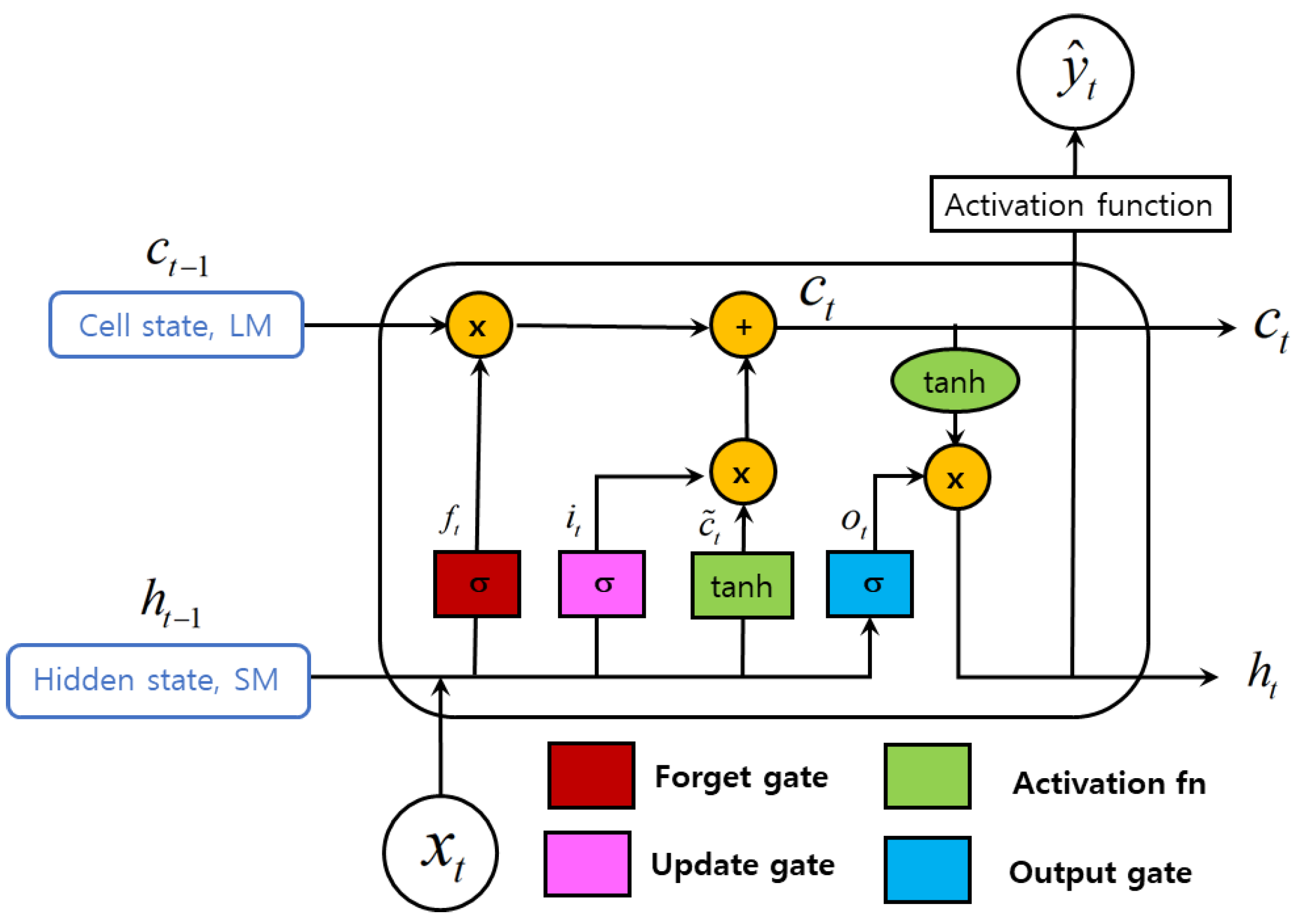
2.3. Deep Learning Model

In time-series forecasting problems, traditional statistical methods have been reported to outperform complex methods, such as MLP, CNN, and RNN [24]. However, machine learning and deep learning are expected to outperform statistical methods in many predictive modeling problems [25]. Researchers are competing to conduct various application studies. In this study, LSTM, among artificial neural network structures, was used for heat flux modeling. The main characteristics and advantages and disadvantages of this LSTM are briefly described. The key idea of LSTM is that the degree of opening and closing of the input gate and output gate at each moment determined by learning can be adjusted in the range of 0 to 1. A LSTM neural network is a type of recurrent neural network (RNN) that can learn long-term dependencies between time-steps in sequence data. LSTM’s memory blocks are connected to each other by hidden nodes, and the output of the memory blocks can go into input gates and output gates. LSTMs can learn the short- and long-run dependencies of a problem and can handle the vanishing gradient problem, which most RNN architectures struggle with. It is very suitable for indoor temperature modeling because it includes both low-speed and high-speed movement phenomena [26].
A cell, the main information processing unit of an LSTM, has several gates that maintain and control the flow of information for sequences of arbitrary length. A feature of this cell is that LSTMs can determine whether information is useful in the long run or in the short run, making it suitable for sequential problems. An LSTM cell can be defined as follows [9,18].
f t = σ ( W f [ h t 1 , x t ] + b f )
i t = σ ( W i [ h t 1 , x t ] + b i )
c ˜ t = tanh ( W c [ h t 1 , x t ] + b c )
c t = f t c t 1 + i t c ˜ t
o t = σ ( W o [ h t 1 , x t ] + b o )
h t = o t tanh ( c t )
where x and h are the input state and hidden state, respectively; t is the current time-step; ⊙ is the Hadamard product; and σ is the sigmoid activation function. c ˜ t , f t , i t , and o t are the current state cell, forget, input, and output gates, respectively, and W and b denote learnable weights and biases, respectively. Figure 2 shows the internal structure of an LSTM cell to intuitively understand the flow of information.
The ultimate goal of machine learning is to find the optimal function that maps the input data to the measured output values and, consequently, the optimal parameters that minimize the error between the model output data and the measured output values.
In this study, the bi-directional long short-term memory (BiLSTM) network architecture is used for time-series data, and a feature matrix is created by considering the time delay of features. Including lagged input vectors allows the model to learn different dynamics of the system that may occur in different time periods. Choosing too small a lag can reduce the comprehensiveness of the learned dynamics, while too many lags needlessly increase it and can lead to overfitting.
As a structural detail of BiLSTM, this study used 2 hidden layers and 60 time-step delays for each feature. Each previous state is connected to an individual LSTM cell, resulting in a layer of 60 cells with a channel for each function. We then deepened the LSTM network into two layers by modifying the replicas of these layers. Finally, we flatten the output of the LSTM layer and use the fully connected layer to obtain a single prediction. The max epoch is 200, the mini-batch size is 128, the number of neurons in the first hidden layer is 120, the number of neurons in the second hidden layer is 80, the dropout is 0.5, and the learning algorithm is Adam.
The method for comparing and evaluating the performance of the deep learning architecture described above is defined and used in various ways [7]. Typically, R2, RMSE, and MAE error metrics are expressed as formulas and defined as follows.
R 2 = 1 ( i = 1 m ( y i y ^ i ) 2 i = 1 m ( y i y ¯ i ) 2 )
R M S E = i = 1 m ( y i y ^ i ) 2 m
M A E = 1 m i = 1 m ( y i y ^ i ) 2
where y ^ and y are the model predicted and actual outputs, respectively; y ¯ is the average of the outputs; and m is the number of samples.

3. Results and Discussion

3.1. Measurement Data and Analysis

Physical quantities were measured under ideal conditions in the model room of the Engineering Building. The data measured by installing temperature and heat flux sensors on the inside and outside of the sample room, fan coil outlet, and north-facing multi-glass windows were analyzed. First, the overall heat transfer coefficient of a building component in the unsteady state can be obtained according to the international standard ISO 9869-1:2014. This standard presents average value calculation methods and dynamic calculation methods for data analysis methods. If there is no phase change material, or the heat storage effect is not large, the heat flux and indoor/outdoor temperature can be measured and calculated using Equation (1). The indoor/outdoor convective heat transfer coefficient required here varies greatly depending on the shape of the environment, and various relationships exist. However, in the case of buildings, h i = 9.30 W/(m2∙K) and h o = 23.26 W/(m2∙K) were used as empirical approximations [27]. In addition, the ISO standard recommends a measurement time of at least 72 h and an analysis error of 5% or less in the consideration of thermal inertia in the case of wall structures. The overall heat transfer coefficient was calculated according to the international standard ISO 9869-1:2014. The U value of the multilayer glass window with anti-reflective coating was 1.84 W / ( m 2 K ) , with an error of 3.4% (Figure 3).
The temperature in the laboratory, roughly regulated by a central plant control system, could also be mildly tuned by a local heater. The air flow rate could also be set by the switch in the fan coil unit (FCU). The air temperatures both inside and outside the room were measured with sensors placed near the center and edges of the walls. Since the room was empty, the impact of occupant movements was negligible. Instead of measuring scattered insolation indirectly, illuminance was measured and considered to improve future prediction accuracy.
Measurements were made every 1-s interval over approximately 7 days, and thereby, a total of 592,124 samples were collected. Detailed information on the measured variables and statistics is summarized in Table 1. Data subsampling was performed at multistep time intervals of 1, 60, 180, 300, 600, 900, 1800, and 3600 s. The heat flux measured through multiple windows is the model’s output variable for prediction. The variable profile is visualized and presented in the Supplementary Material Figure S1. Since the heat flux dynamics are repeatable, the previous values of the output variables were used as features of the model. We split the first 80% of the data into a training set and the remaining 20% into validation and test data.
Figure 4 shows the results obtained using a wavelet transform to extract and visualize features from the measured heat flux. It is obtained using the analytic Morse wavelet with the symmetry parameter, gamma (γ), equal to 3. The minimum and maximum scales are determined automatically based on the energy spread of the wavelet in frequency and time [28]. It shows a more accurate representation of the signal by using L1 normalization. In this three-dimensional scalogram, it can be seen that when the frequency is very low, the magnitude is maintained at a high level regardless of time. In the case of time greater than 440,000 s and frequency greater than 10−3 Hz, the magnitude is apt to be very low, and this specific case mainly happened during the weekend. For the case of the frequency from 0.001 to 0.1 Hz, the time-dependent characteristics are relatively high. It is estimated that peaks in power levels are time-dependent, but are generated at approximately 3.377 × 10⁻⁶ Hz (82.2 h), 1.182 × 10⁻⁵ Hz (23.5 h), 2.364 × 10⁻⁵ Hz (11.8 h), 3.377× 10⁻⁵ Hz (8.2 h), 4.56 × 10⁻⁵ Hz (6.1 h), 5.742 × 10⁻⁵ Hz (4.8 h), 6.418 × 10⁻⁵ Hz (4.3 h), etc. from the Fourier transform. Note that the frequency information can also be obtained conceptually by integrating the temporal spectral function g(f,t) with respect to time. At frequencies higher than 0.2 Hz (5 s), power levels were found to be low and insignificant. Therefore, the characteristics of the system can be understood, and it is considered appropriate to adopt the control-monitoring interval of the system as 1 s, 60 s, 180 s, 300 s, etc. through subsampling. Considering the thermal conductivity of glass, the reason for the large system characteristic time is considered to be due to the effect of the air layer insulation inside the multi-window room and the thermal mass of concrete slab on the ceiling and floor.

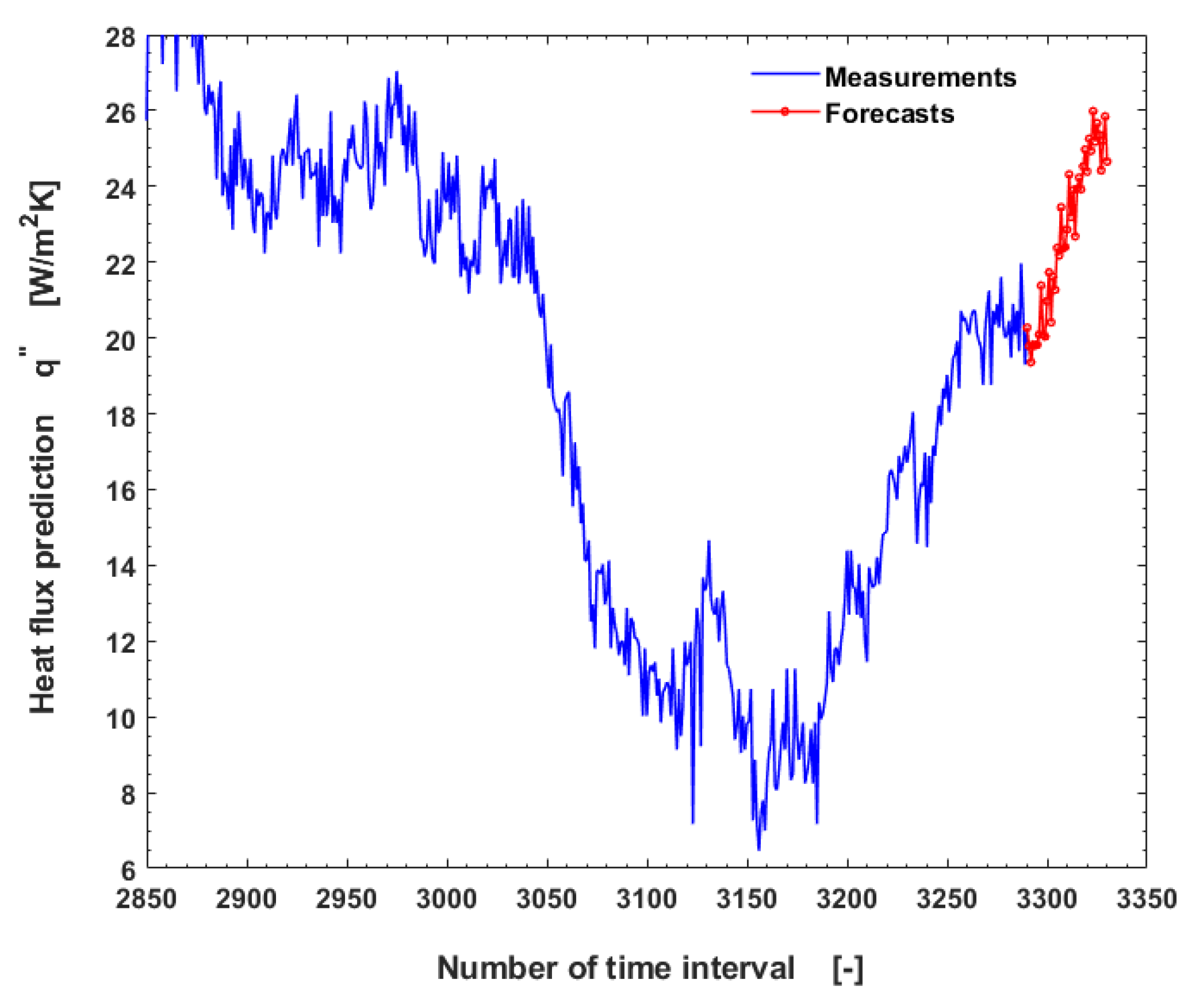
3.2. LSTM Neural Networks

The LSTM neural network was used for prediction of heat flux in this study, and the configuration of the neural network is 60-120-80-1. The input size depends on the network architecture. We apply 60 time-step lag observations for every function and output, and train it to predict the heat flux at the next time-step. Performance evaluation was performed on training, testing, and full sets. To evaluate the short-term predictive ability of the model, we used 40 prediction horizons.
Figure 5 shows the heat flux measurement and deep learning prediction, along with lines splitting the training and test data. In Figure 5a–h, we feel that the predictions of all measuring time intervals are plausible, except for 3600 s. It shows that the shorter the subsampling time interval, the higher the prediction accuracy. It can be seen that the trained and test data-sets agree very well with the outputs when the multistep time interval tmsi is 600 s or less.
Figure 6 is the error histogram for all training and test data over several multistep time intervals. When the tmsi was 1 s, the mean and standard deviation of errors were good at −0.0641 and 0.6771, respectively. Good symmetry was shown when the subsampling time interval tmsi was 180 s or less.
Figure 7 shows the regression graph of heat flux targets and predictions by fitting all data. When the multistep time interval is 180 s or less, the coefficient of determination R2 for the test data is good at 0.918 or more. When the multistep time interval tmsi is 600 s, the decision R2 of the entire data is 0.7 or more (Table 2).
The control and monitoring time intervals are critical in real plant operation and management. To investigate the effect of the sampling rate on predictions, the data are extracted by subsampling, as was described previously. That is, the data for tmsi at 1800 s are a subset of that of 60 s because the sample pick-up is performed at multiples of 60. For every target and prediction of heat flux, several error metrics, such as R2, RMSE, and MAE, were calculated [7]. In order to understand the effect of the sampling rate on prediction accuracy, modeling was performed. Various error metric indicators were compared, as shown in Table 2 and Table 3. As expected, when training data are included as a precision measurement index, the index value is higher. Yet, the sensitivity for comparison and differentiation between models is lower. Looking closely at the coefficient of determination R2 for the test data, it can be seen that R2 is higher than 0.757 when the heat flux measurement interval is less than 180 s, and then drops to less than 0.6 when it is greater than 900 s. Therefore, it can be seen that it is desirable to maintain the sampling interval at a level of at least 180 s or less, if possible. Even if the window area is small and the indoor temperature change is relatively slow compared to the heat flux change, it is desirable to keep it within 1000 s. For other error metric indicators (MAE, MAPE, MSE, and CVRMSE) shown in Table 3, they increase as the multistep time increases. From an instrument control point of view, the faster the sampling rate, the better. It should be noted that the computational cost increases significantly as the sampling rate increases. Therefore, the exponentially increasing computation time must be taken into account when performing dynamic simulations, as well as real machine controls. This shows that the LSTM network structure can be usefully utilized for heat flux modeling. This allows transient physical characterization of pre-installed building components, which was difficult to access with conventional steady-state methods.
To forecast or predict future outcomes, modeling was performed over the prediction horizon. Figure 8 shows a short-term forecast of the future output for a prediction horizon of 40, i.e., 40 steps, after predicting the test data. In this process, the model uses the results to make further predictions for the future. In general, for one-step ahead predictions, the model performs satisfactorily for target predictions, but care must be taken when increasing the prediction horizons. In Figure 8a–h, we feel that the predictions of all measuring time intervals are plausible, apparently in spite of very low R2. The forecasts behave similarly or differently over the sampling interval. Figure 9 shows a typical, right, enlarged view of Figure 8c for the multistep time interval of 180 s. Intuition and experience are still helpful in the data-driven engineering. We can presume a little bit because it starts around 21:00 on Sunday. Heat flux has highly sensitive and repeatable dynamics, so previous values have a significant impact on future predictions. As the time of the prediction horizon increases, deviations between measured and predicted values are inevitable in the next step due to an error accumulation effect similar to extrapolation [29]. Even if we can challenge to predict the future, the exact details are in the realm of the gods.
We have also used other models, such as multilayer perceptron (MLP) and hybrid convolutional neural network-long short time memory (CNN-LSTM) models [25,26]. The results are shown in Table 4. For the hybrid CNN-LSTM model, the performance index is unexpectedly similar and not the best [13], but the computation time is about 10 times longer [18]. Further investigations are necessary, and details will appear later in another article.
On the other hand, an analysis was performed on a multivariable input single-variable output system (MISO) considering inputs such as the indoor temperature, outdoor temperature, indirect illuminance, and outlet air temperature of the fan coil units, in addition to heat flux on the window [30]. Although not optimized, Table 5 shows the compared results using the same network configuration. For the multivariate models, computing time increased significantly, and data variance was slightly greater. As can be seen from the table, the overall error metrics show almost similar results. Detailed results are presented in the supplementary material. In future studies, it is necessary to seek ways to solve the limitations of the number of data with various approaches, increase the long-term and short-term prediction accuracy, improve the accuracy, and reduce the calculation time used for system control.

4. Conclusions

In this study, the BiLSTM structure was used to predict the heat flux of multiple windows. A data-set consisting of various physical quantities was measured at intervals of 1 s, using heat flux sensors and temperature sensors in the test room to obtain time-series data. As a result of calculating the overall heat transfer coefficient according to the international standard ISO 9869-1:2014, the U value of the multi-window with anti-reflection coating was 1.84 W/(m2∙K). Features were extracted from the measured data using a wavelet transform and visualization. To understand the thermal behavior of multiple windows, we constructed the BiLSTM network configurations, trained and tested the measured heat flux, and predicted future values. Error metrics were used to evaluate the performance of the neural network structures over multistep time intervals and to provide reasonable baseline values for monitoring and control time intervals. The BiLSTM structure has been shown to be useful for heat flux predictions. It is found that the multistep time interval for control and monitoring is preferably no more than 240 s. The coefficient of determination (R2, R-squared) is recommended for evaluating the performance of networks. Forecasts or future prediction in short time behave similarly or differently over the sampling interval. Intuition and experience are still helpful in the data-driven engineering. Transient measurement of building components has been found to be useful for analyzing the thermal behavior of a building. Multivariate analysis with several input variables was also performed, and similar results were obtained.

Supplementary Materials

The following supporting information can be downloaded at: https://www.mdpi.com/article/10.3390/buildings13030707/s1, Figure S1: Data-set for multivariate LSTM neural network analysis; Figure S2: Regression evaluation for target and prediction values using eight inputs (multistep time interval = 60 s, LSTM 2 layers); Figure S3: Variation of target and predicted heat fluxes for test data-set (multistep time interval = 60 s, LSTM 2 layers).

Author Contributions

Conceptualization, B.K.P.; data curation, C.-J.K.; formal analysis, B.K.P.; funding acquisition, B.K.P.; investigation, C.-J.K.; methodology, C.-J.K. and B.K.P.; project administration, B.K.P. and C.-J.K.; validation, B.K.P.; writing—original draft B.K.P.; writing—review and editing, C.-J.K. All authors have read and agreed to the published version of the manuscript.

Funding

This research was supported by Ministry of Land, Infrastructure and Transport of the Korean government through Korea Agency for Infrastructure Technology Advancement(KAIA) Grant 22TBIP-C161109-02 and Grant 22CTAP-C163752-02.

Data Availability Statement

Not applicable.

Conflicts of Interest

The authors declare no conflict of interest. The authors identify and declare no personal circumstances or interest that may be perceived as inappropriately influencing the representation or interpretation of the research results. The funders had no role in the design of the study; in the collection, analyses, or interpretation of data; in the writing of the manuscript; or in the decision to publish the results.

References

  1. International Energy Agency. Buildings, Energy. Available online: https://www.iea.org/reports/buildings (accessed on 19 January 2023).
  2. Tafakkori, R.; Fattahi, A. Introducing novel configurations for double-glazed windows with lower energy loss. Sustain. Energy Technol. Assess. 2021, 43, 100919. [Google Scholar] [CrossRef]
  3. ASHRAE. Handbook Fundamentals, SI, International Edition, 1997; ASHRAE Handbook—HVAC Applications; ASHRAE Parsons: Peachtree Corners, GA, USA, 2007. [Google Scholar]
  4. Lu, C.; Li, S.; Lu, Z. Building energy prediction using artificial neural networks: A literature survey. Energy Build. 2022, 262, 111718. [Google Scholar] [CrossRef]
  5. Wang, Z.; Chen, Y. Data-driven modeling of building thermal dynamics: Methodology and state of the art. Energy Build. 2019, 203, 109405. [Google Scholar] [CrossRef]
  6. Rouchier, S. Solving inverse problems in building physics: An overview of guidelines for a careful and optimal use of data. Energy Build. 2018, 166, 178–195. [Google Scholar] [CrossRef]
  7. Bourdeaua, M.; Zhaia, X.Q.; Nefzaouib, E.; Guo, X.; Chatellier, P. Modeling and forecasting building energy consumption: A review of data-driven techniques. Sustain. Cities Soc. 2019, 48, 101533. [Google Scholar] [CrossRef]
  8. Kirubakaran, V.; Sahu, C.; Radhakrishnan, T.K.; Sivakumaran, N. Energy efficient model based algorithm for control of building HVAC systems. Ecotoxicol. Environ. Saf. 2015, 121, 236–243. [Google Scholar] [CrossRef]
  9. Ming, W.; Sun, P.; Zhang, Z.; Qiu, W.; Du, J.; Li, X.; Zhang, Y.; Zhang, G.; Liu, K.; Wang, Y.; et al. A systematic review of machine learning methods applied to fuel cells in performance evaluation, durability prediction, and application monitoring A systematic review of machine learning methods applied to fuel cells in performance evaluation, durability prediction, and application monitoring. Int. J. Hydrogen Energy 2023, 48, 5197–5228. [Google Scholar]
  10. Brunton, S.L.; Kutz, J.N. Data-Driven Science and Engineering—Machine Learning, Dynamical Systems, and Control, 2nd ed.; Cambridge University Press: Cambridge, UK, 2022. [Google Scholar]
  11. Roman, N.D.; Bre, F.; Fachinotti, V.D.; Lamberts, R. Application and characterization of metamodels based on artificial neural networks for building performance simulation: A systematic review. Energy Build. 2020, 217, 109972. [Google Scholar] [CrossRef]
  12. Tien, P.W.; Wei, S.; Darkwa, J.; Wood, C.; Calautit, J.K. Machine Learning and Deep Learning Methods for Enhancing Building Energy Efficiency and Indoor Environmental Quality—A Review. Energy AI 2022, 10, 100198. [Google Scholar] [CrossRef]
  13. Chen, Z.; Xiao, F.; Guo, F.; Yan, J. Interpretable machine learning for building energy management: A state-of-the-art review. Adv. Appl. Energy 2023, 9, 100123. [Google Scholar] [CrossRef]
  14. Noye, S.; Martinez, R.M.; Carnieletto, L.; DeCarli, M.; Aguirre, A.C. A review of advanced ground source heat pump control: Artificial intelligence for autonomous and adaptive control. Renew. Sustain. Energy Rev. 2022, 153, 111685. [Google Scholar] [CrossRef]
  15. Mohanraj, M.; Jayaraj, S.; Muraleedharan, C. Applications of artificial neural networks for refrigeration, air-conditioning and heat pump systems—A review. Renew. Sustain. Energy Rev. 2012, 16, 1340–1358. [Google Scholar] [CrossRef]
  16. Attoue, N.; Shahrour, I.; Younes, R. Smart building: Use of the artificial neural network approach for indoor temperature forecasting. Energies 2018, 11, 395. [Google Scholar] [CrossRef] [Green Version]
  17. Kreuzer, D.; Munz, M.; Schlüter, S. Short-term temperature forecasts using a convolutional neural network—An application to different weather stations in Germany. Mach. Learn. Appl. 2020, 2, 100007. [Google Scholar] [CrossRef]
  18. Elmaz, F.; Eyckerman, R.; Casteels, W.; Latré, S.; Hellinckx, P. CNN-LSTM architecture for predictive indoor temperature modeling. Build. Environ. 2021, 206, 108327. [Google Scholar] [CrossRef]
  19. Rouchier, S.; Rabouille, M.; Oberlé, P. Calibration of simplified building energy models for parameter estimation and forecasting: Stochastic versus deterministic modelling. Build. Environ. 2018, 134, 181–190. [Google Scholar] [CrossRef]
  20. Wu, W.; Wang, J.; Huang, Y.; Zhao, H.; Wang, X. A novel way to determine transient heat flux based on GBDT machine learning algorithm. Int. J. Heat Mass Transf. 2021, 179, 121746. [Google Scholar] [CrossRef]
  21. Biddulph, P.; Gori, V.; Elwell, C.A.; Scott, C.; Rye, C.; Lowea, R.; Oreszczyn, T. Inferring the thermal resistance and effective thermal mass of a wall using frequent temperature and heat flux measurements. Energy Build. 2014, 78, 10–16. [Google Scholar] [CrossRef] [Green Version]
  22. Park, B.K.; Cho, D.W.; Shin, H.J. Energy Analysis for Variable Air Volume System. Mag. Soc. Air-Cond. Refrig. Eng. Korea 1988, 17, 575–582. [Google Scholar]
  23. ISO 9869-1; Thermal Insulation—Building Elements—In-Situ Measurement of Thermal Resistance and Thermal Transmittance. International Standard: Brussels, Belgium, 2014.
  24. Makridakis, S.; Spiliotis, E.; Assimakopoulos, V. Statistical and Machine Learning forecasting methods: Concerns and ways forward. PLoS ONE 2018, 13, e0194889. [Google Scholar] [CrossRef] [Green Version]
  25. Ibrahim, B.; Rabelo, L.; Gutierrez-Franco, E.; Clavijo-Buritica, N. Machine Learning for Short-Term Load Forecasting in Smart Grids. Energies 2022, 15, 8079. [Google Scholar] [CrossRef]
  26. Mtibaa, F.; Nguyen, K.-K.; Azam, M.; Papachristou, A.; Venne, J.-S.; Cheriet, M. LSTM-Based indoor air temperature prediction framework for HVAC systems in smart buildings. Neural. Comput. Appl. 2020, 32, 17569–17585. [Google Scholar] [CrossRef]
  27. Lavine, A.S.; Bergman, T.L.; Incropera, F.P.; DeWitt, D.P. Fundamentals of Heat and Mass Transfer, 8th ed.; Wiley: Hoboken, NJ, USA, 2019. [Google Scholar]
  28. Mathlab. Deep Learning Toolbox; Mathoworks: Natick, MA, USA, 2022. [Google Scholar]
  29. Chapra, S.C.; Canale, R.P. Numerical Method for Engineers, 4th ed.; McGraw Hill: New York, NY, USA, 2002. [Google Scholar]
  30. Brownlee, J. Deep Learning for Time Series Forecasting—Predict the Future with MLPs, CNNs, and LSTMs in Python; Machine Learning Mastery: San Juan, PR, USA, 2020. [Google Scholar]
Figure 1. Photograph (a) and schematic (b) of the test room.
Buildings 13 00707 g001
Figure 2. Diagram of LSTM cell structure (operations are marked by yellow color).
Buildings 13 00707 g002
Figure 3. Thermal measurements and U-value analysis for the North window based on ISO 9869-1: 2014.
Buildings 13 00707 g003
Figure 4. Three-dimensional scalogram showing heat flux features.
Buildings 13 00707 g004
Figure 5. Evaluation of output graph for all data using LSTM model.
Buildings 13 00707 g005aBuildings 13 00707 g005b
Figure 6. Error histogram for all data using LSTM model.
Buildings 13 00707 g006aBuildings 13 00707 g006b
Figure 7. Evaluation of regression graph for all data using LSTM model.
Buildings 13 00707 g007aBuildings 13 00707 g007b
Figure 8. Forecasts (future prediction) on prediction horizon 40 using LSTM model.
Buildings 13 00707 g008aBuildings 13 00707 g008b
Figure 9. Right enlarged view of Figure 8c, multistep time interval of 180 s.
Buildings 13 00707 g009
Table 1. Statistical summary of the data-set.
MinimumMaximumMeanStandard Dev.
Heat_Flux−3.1658.5022.458.18
T117.0027.0021.231.86
T22.7518.888.843.39
T3_116.0048.7523.367.38
T3_215.0027.0018.802.35
T3_36.7523.0011.843.32
T3_416.0026.0020.421.83
Ev_Flex720.09201.6030.9241.99
Table 2. Comparison of calculated error metrics between test and all data for various multistep time intervals.
tmsiRank CorrelationError-MeanError-StdR-SquaredRank CorrelationError-MeanError-StdR-Squared
allallallalltesttesttesttest
10.99625−0.064090.67710.993290.99503−0.05920.51580.9936
600.968810.218591.83210.947610.942320.10821.95280.9018
1800.97433−0.211601.72450.955800.87300−0.60963.19140.7571
3000.95255−0.138892.29130.923550.78438−0.75414.17310.5557
6000.94454−0.089212.41180.918430.76105−0.14664.07790.6046
9000.90634−0.533803.17760.860690.75344−1.97844.72840.5914
18000.83488−0.869574.84970.696650.73051−2.81454.66130.4865
36000.92751−0.476792.58830.883620.54675−2.38415.4823-
Table 3. Calculated error metrics for various multistep time intervals (tmsi) in test data.
tmsiMAEMAPEMSECVRMSESSEMBENMBEMRE
10.3979732.0796770.26954411.59130131917.574−0.0591680.2949330.002949
601.2793736.9107303.82316243.8994787531.6300.1081670.5452430.005452
1802.27692911.97271010.54083271.5427856809.377−0.6096292.9602120.029602
3002.44438413.09541312.26793277.3309867925.084−0.5301712.5843530.025843
6002.91206915.00225817.93765893.0621566870.123−0.7541233.6410180.036410
9003.08905716.36696216.56110090.1133423063.803−0.1466560.7191030.007191
18003.92245216.59594926.085100107.813363130.211−1.978366−8.8157540.088157
36004.25476418.24489429.246843110.984421579.329−2.81448411.8534270.118534
Table 4. Error metrics comparison for typical models.
(tmsi = 60 s)RsquaredRMSEMAEMAPEMSECVRMSESSEMBENMBEMRE
MLP0.92031.8001.2066.523.24340.2466363.3−0.061−0.3020.003
CNN-LSTM0.90462.0271.4357.564.11044.9968063.8−0.337−1.6580.017
Table 5. Performance evaluation of the LSTM model for test data (tmsi = 60 s); LSTM 2 layers.
RsquaredRMSEMAEMAPEMSECVRMSESSEMBENMBEMRE
BiLSTM
(univariate)
0.90181.9551.2796.913.82343.8997531.60.1080.5450.005
BiLSTM
(multivariate)
0.8882.2631.6428.345.12147.92114,717.60.1470.6590.007
Disclaimer/Publisher’s Note: The statements, opinions and data contained in all publications are solely those of the individual author(s) and contributor(s) and not of MDPI and/or the editor(s). MDPI and/or the editor(s) disclaim responsibility for any injury to people or property resulting from any ideas, methods, instructions or products referred to in the content.

