A Case Study of Empirical Validation of EnergyPlus Infiltration Models Based on Different Wind Data

Abstract

Building retrofitting is an efficient means of reducing greenhouse gas emissions. Its first focus is on building façade, as transmission and air leakage are the main sources of energy loss in buildings. Nowadays, building modellers cannot easily implement envelope air leakage and assume constant values, which results in erroneous energy estimates. Additionally, in energy simulations, a weather file is usually inserted with measurements provided by a weather station. In this study, we revealed the use of wind data from the weather file (herein as global wind) to calculate the infiltration of a test case in Spain, using the three algebraic equations of EnergyPlus. Furthermore, four other wind data were applied: eastbound and westbound winds from the weather file and two from in situ measurements (on the southeast and on the northwest façades). The fifteen combinations of the three infiltration models and the five wind data were empirically evaluated, using the tracer gas results performed during three different periods. The combinations were validated according to the American Society for Testing Materials D5157 standard criteria, and the best and the only ones that complied with the standard were those using the wind data from the southeast in situ sensor and the west wind from the weather station. The global wind was not able to generate accurate infiltration models, which raises doubts about its use in the highly-time calibration of energy models. However, its disaggregation was a cost-effective strategy to estimate the infiltration of this case study.

1. Introduction

In 2020, the European Union (EU) provided an unprecedented response to the coronavirus crisis that hit Europe and the world through hlNext Generation EU (NGEU): a temporary instrument called Recovery and Resilience Facility (RRF). The RRF makes EUR 750 billion (in 2018 prices) in grants to ease the recovery actions and investments carried out by Member States [1]. The main goal of the RRF is to reduce the social and economic footprint created by the pandemic and to make European societies and economies more resilient, sustainable, and ready for a new paradigm based on green and digital transitions. A minimum of 30% of expenditure should be dedicated to climate investment and reforms [2]. Among the flagship areas, buildings renovation appears as the most crucial, because building retrofitting is probably the most cost-effective way of cutting down greenhouse gas emissions [3].

Furthermore, the European Union proposed a set of directives to eradicate inefficient buildings, by enforcing the Energy Performance of Buildings Directive (EPBD). In this framework, building energy retrofit projects will rely on using digital twins, which can be created by using building information modelling (BIM) technology, followed by a building energy model (BEM) to quantify energy savings. For this purpose, the interoperability between BIM and BEM should be considered, in order to guarantee the confidence of investors in the energy efficiency sector [4]. However, BEM requires adjustments of input parameters that are unknown and difficult to measure, leading to high unpredictability in energy savings. Therefore, the limitations in the analysis of building energy retrofit are mainly due to the lack of accuracy of the model.

1.1. Background and Motivation

Retrofit projects typically use a calibrated BEM to ensure that building systems are properly modeled. There are challenges in the calibration process for the measurement and verification of energy savings, which can be based on mathematical algorithms and physical-based models and are evaluated according to uncertainty analysis [5,6,7]. As stated by the ASHRAE Handbook: Fundamentals: SI edition (2017) [8], several difficulties prevent achieving a calibrated simulation [9,10,11,12]. One of them is the method used to measure the input parameters needed for the simulation, i.e., infiltration values [13,14,15,16].

Infiltration is also known as the flow of outdoor air into a building through unintentional openings. Similar to natural ventilation, infiltration is driven by the pressure differences across the envelope caused by air and wind density variability generated by the temperature differences between indoor and outdoor air. For that reason, infiltration has two components: stack pressure and wind pressure. Stack pressure is the hydrostatic pressure produced by the mass of a column of air inside or outside a building [17]. When wind impinges on a façade, it creates a distribution of static pressures that depends on the wind speed, wind direction, surface orientation, air density, and surrounding conditions [18]. Moreover, if there is infiltration in a building envelope, it could affect the heating and cooling loads. If the outside air entering the building is cold, the heating load could increase by 13% to 30%. On the other hand, if it is warm, the cooling load could increase by 4% to 14% [19,20]. Furthermore, some studies estimated that air leakage could be responsible for 50% of energy loss [21,22]. In the current context, where regulations are being created to reduce carbon emissions [23], it is relevant to control any cause of increasing building loads, one of the most important of which is leakage airflow, and, therefore, its precise measurement and correct input in BEM software should be carried out.

1.2. Infiltration Modelling

Detailed models for air leakage can be produced by using multizone airflow or CFD software. In EnergyPlus, the AirFlowNetwork (AFN) model can be used to determine model infiltration and mixing airflow between zones with or without HVAC operation. It presents three empirical equations to calculate infiltration: ZoneInfiltration:DesignFlowRate, ZoneInfiltration:FlowCoefficient, and ZoneInfiltration:EffectiveLeaka-geArea. In addition to facilitating more accurate calculations of wind-driven infiltration, EnergyPlus calculates the wind speed as a function of height by using the input or default wind speed profile coefficients [24].

CONTAM is another multizone simulation software, which was developed at the National Institute of Standards and Technology (NIST) and is widely accepted to estimate infiltration [25]. In CONTAM models, it is possible to implement wind direction and wind speed, ideally for each thermal zone. Therefore, another possibility is coupling CONTAM with EnergyPlus (EP), but it can be a cumbersome process, and the main limitation of this co-simulation technique is related to the synchronisation time-step size of the quasi-dynamic method [26]. Additionally, when translating these results to EnergyPlus, infiltration rates are averaged over the entire exterior surface area, as was explained by Ng et al. [25,27]. Empirical approaches simplify multizone building airflow models and represent cost-effective solutions for non-expert users.

The wind is a key factor in the generation of air leakage, and since the EP empirical equations consider the wind speed data to quantify infiltration, it is important to analyse which wind speed values should be applied. In some studies, authors installed a dedicated weather station on the roof of their test case to use actual weather data in modelling, as is the case in Shrestha et al. and Bae et al. [28,29]. In contrast, Taddeo et al. [16] collected the wind speed data from a weather station 1 km far from their test space. Their wind speed values were corrected according to the height of the building. Winkler et al. [30] evaluated EnergyPlus AFN models for residential infiltration. They determined five cases, and in each, they changed the test conditions. In relation to the wind speed, in the second and fifth cases, they used a typical meteorological year (TMY) wind speed data, while in the first and third cases, they applied a wind speed value of 5 m/s, and in the fourth case, 0 m/s. The aim of their study was to compare EP AFN models with CONTAM and building energy optimisation (BEopt) [31] models, but they did not use in situ wind speed data, and it was not in their scope to empirically assess the models.

1.3. Tracer Gas Technique

The most accurate way to determine a building’s infiltration rate is to measure it. According to ASHRAE [8], tracer gas measurement is the reference technique. There are procedures (e.g., the Standard ASTM E741 test method [32]) that use gas to label indoor air, as stated by Sherman in different works [33,34,35]. There are three methods for tracer gas test: constant injection, constant concentration, and concentration decay; the latter is the easiest to implement [36].

As described by Cui et al. [37], the concentration decay method consists of injecting a dose of CO${}_2$ and mixing it into the room. The decay method is based on the assumptions that (1) the background concentration is known, (2) infiltration out of the building is the main way of removing the CO${}_2$ from the room, and (3) the CO${}_2$ concentration within the room should be uniform. The decrease in CO${}_2$ is recorded during a given period.

1.4. Contribution and Originality of the Research

This preliminary study aims to reduce the uncertainty of infiltration in the building energy model calibration, using only the EnergyPlus infiltration objects and different wind data. Although many studies evaluate wind-driven infiltration modelling, as far as the authors know, none of the published validation reports on air leakage empirically compare different wind data applied with the EnergyPlus infiltration models, with one of the wind data being measured in situ. In this study, we revealed the use of the wind data from the weather file (hereafter, the global wind) against four other wind data to estimate the infiltration of a test room in an apartment in Spain. The global wind is usually applied in energy simulations. There is a general consensus that EP only accounts for wind speed and does not have a wind direction component in the infiltration objects [38]. Therefore, we focused on the global wind and disaggregated it into two types of data: the eastbound wind and the westbound wind. In addition, we used the wind data recorded with sensors in situ: one on the southeast façade and the other on the northwest façade. We applied the five wind data to the three infiltration models of EnergyPlus, resulting in fifteen combinations, to verify which of these most accurately represented the infiltration of the test space.

We performed a tracer gas test based on the concentration decay method [37], to measure infiltration and empirically validate the results. CO${}_2$ was chosen as tracer gas because it complies with the desirable qualities such as detectability, non-reactivity, and non-toxicity at low concentrations, and it is well stirred with air (similar density), so it should be differentiated from other components of air [39]. This in situ experiment was performed over 31 days in three different periods (summer, winter, and spring), and a total of 48.439 time-steps of one-minute data of CO${}_2$, wind speed, and temperature were recorded.

The results were statistically verified. We calculated the standard deviation values for the analysis of the measurements. In addition, we assessed the accuracy of the 15 combinations with the mean bias error (MBE) values [40] and presented in Equation (A4). Then, we evaluated their correlation between the measured and predicted values according to the Standard Guide for Statistical Evaluation of Indoor Air Quality Models (ASTM D5157) requirements [41], which is suggested by ASHRAE [8] for the empirical validation of experimental evidence of indoor environment modelling. To the authors’ knowledge, no previous study has ever used all ASTM D5157 requirements to evaluate EP infiltration models.

The remainder of this paper is organised as follows: Section 2 describes the test room, the monitoring system, and the tracer gas experiment; Section 3 explains the method to calculate the air leakage of the test space, and Section 4 presents the MBE and the ASTM D5157 Standard used to evaluate the models. Finally, in Section 5, we analyse the recorded data, and Section 6 shows the results of the fifteen combinations. Section 7 concludes this research.

2. Experimental Procedure

2.1. Test Room and Instrumentation

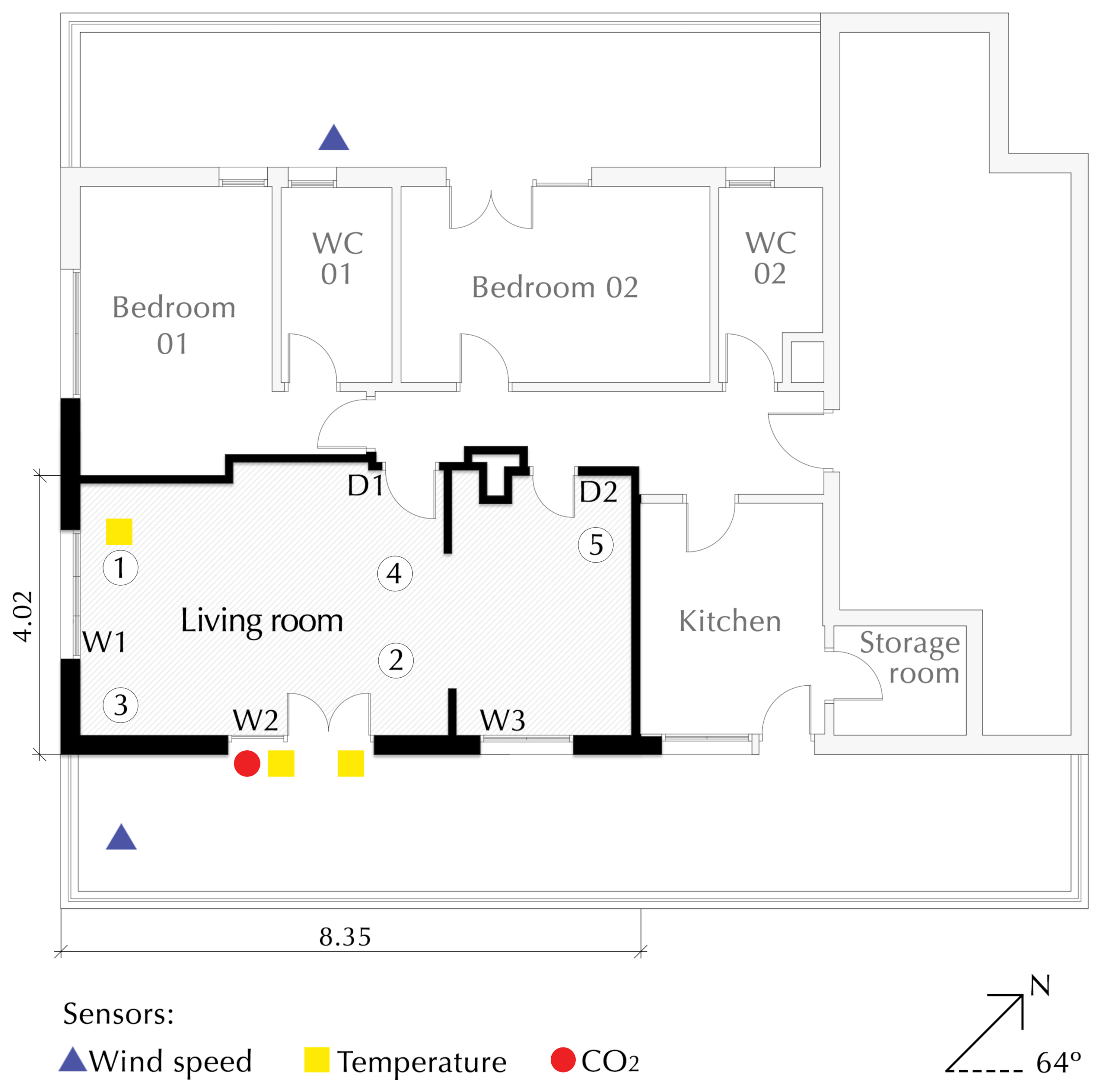
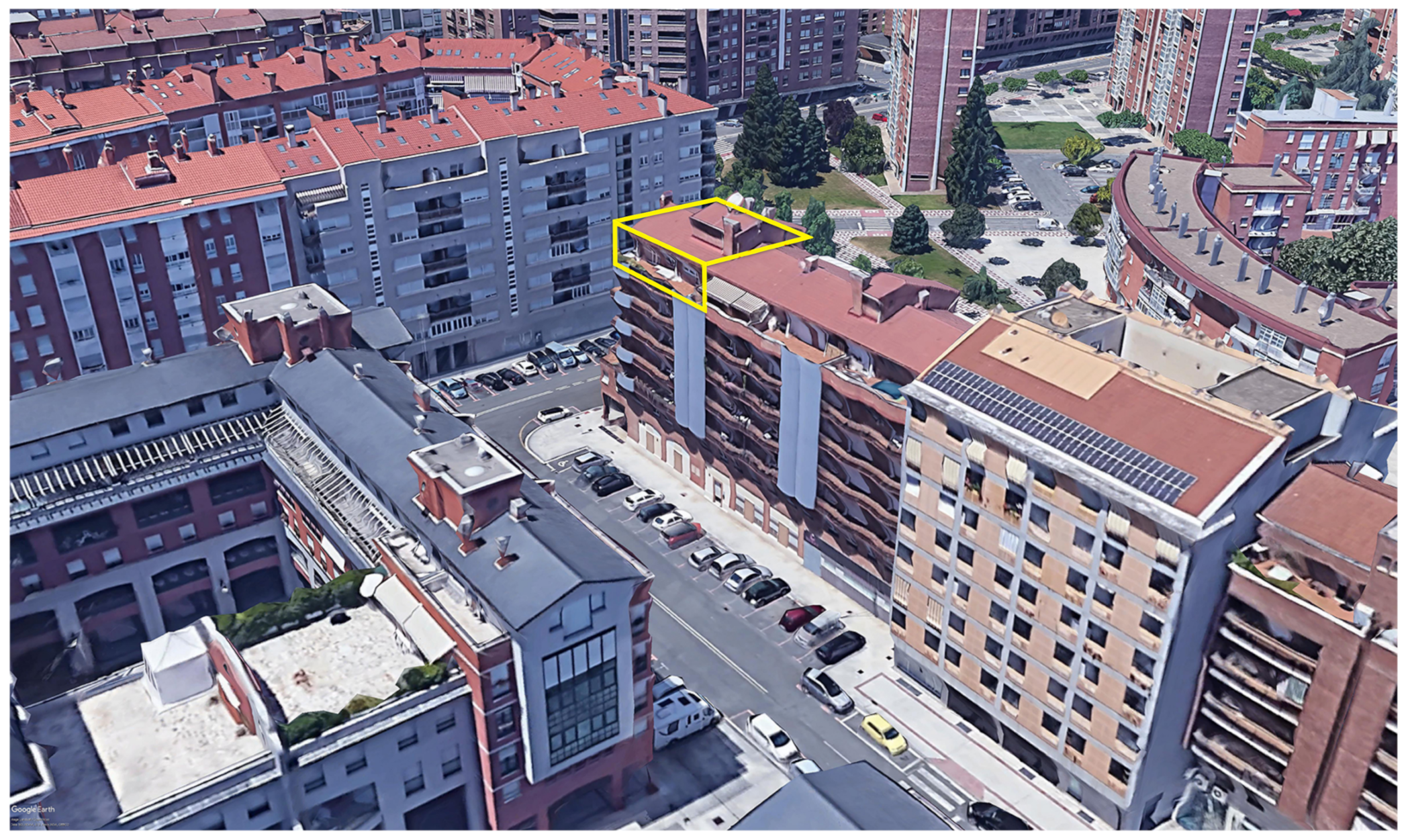
A tracer gas test of the concentration decay method was conducted in the living room of an attic of a seven-story apartment building in Pamplona, Spain (see Figure 1). The room with an area of 29.50 m² has two main façades (southeast and southwest) made of perforated brick of 115 mm, with an air cavity of 30 mm, as well as 50 mm EPS foam, 70 mm hollow brick, and a last layer of gypsum plaster of 15 mm. The interior walls are constructed with gypsum plaster (20 mm), hollow brick (75 mm), and gypsum plaster (20 mm). Figure 2 shows the dimensions of the openings and their position in the room.

The in situ monitoring system consisted of two types of sensors: DELTA (model OHM HD37VBTV.1) and EXTECH (model CO210). Besides the two CO${}_2$ DELTA sensors (ppm) installed in the living room, three CO${}_2$ EXTECH sensors (ppm) were also implemented, in order to verify the homogeneity of the injected gas (see Figure 3 and Figure 4). Both had the same accuracy of ± 50 ppm, but the DELTA sensors were connected to the HOBO management system of the room, making it easier to manage and download their data.

Moreover, two sensors of indoor ambient temperature (°C), model HOBO ZW-006 (with $\pm 2\%$ precision), were installed at different heights (0.80 m and 1.75 m above the ground), and their average was used in the equations.

In relation to weather conditions, a total of five sensors were placed outside the apartment. Two wind speed sensors (m/s) were installed, model AHLBORN FVA 615-2 with ±0.5 m/s accuracy: one at 1.60 m above the ground on the northwest terrace and the other at 1.90 m above the ground on the southeast terrace. The three other sensors were placed 2.32 m above the ground on the southeast façade: one for CO${}_2$ (ppm), model Delta OHM HD37VBTV.1, and two for outdoor ambient temperature (°C), model HOBO ZW-006.

In order to capture the variation in the data as completely as possible, both indoor and outdoor data were recorded at a time-step of one minute.

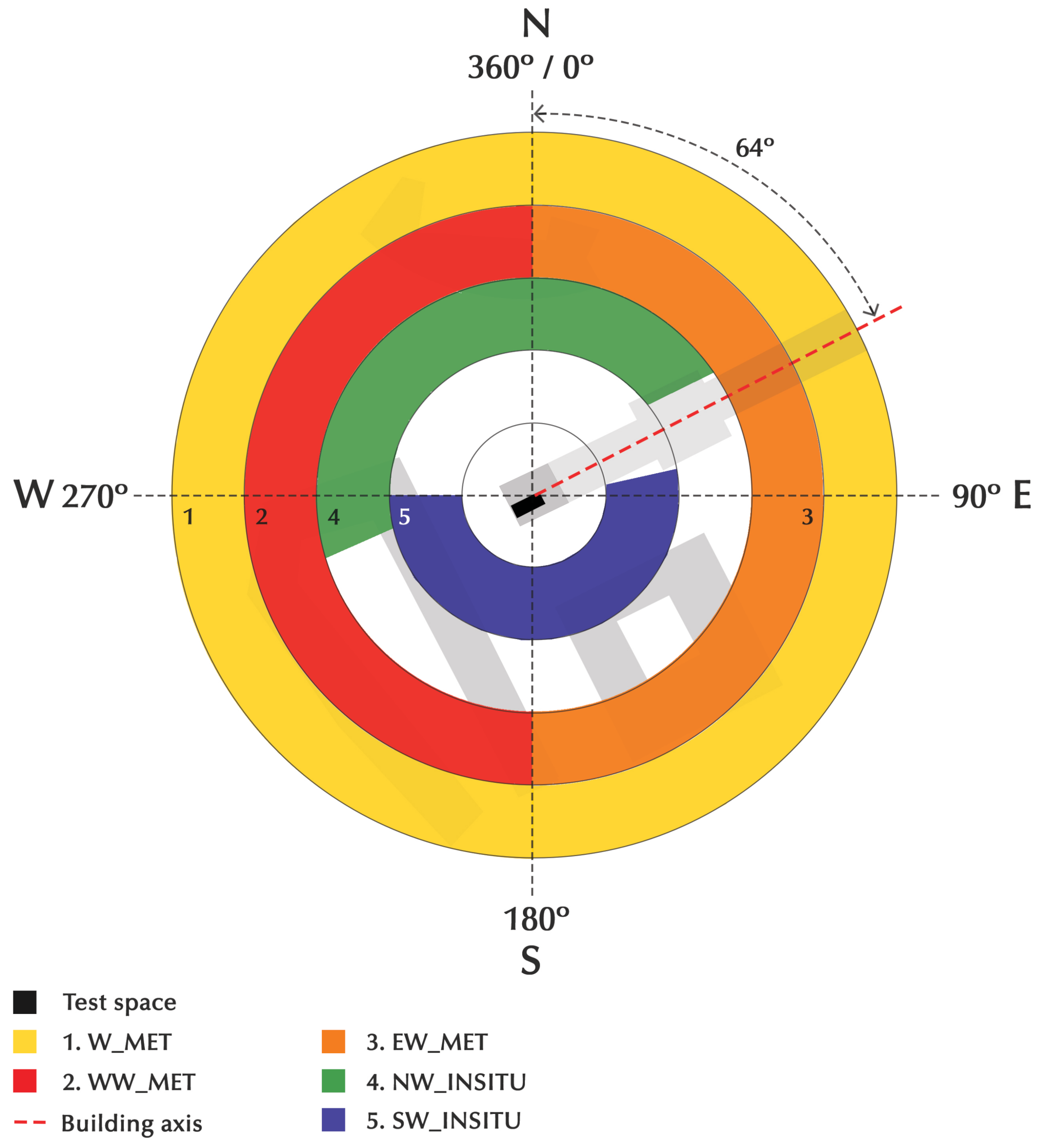
In addition to the in situ data, the wind speeds collected at a weather station were also used. The station was installed on the roof of a commercial building located 2 km away from the test house. Therefore, five different wind data were used to calculate infiltration, and they were organised as explained in Figure 5.

2.2. Tracer Gas Test

The tracer gas concentration decay test was carried out during three different seasons, and its data were organised into three periods, where T represents training, and C represents checking. The first period (P_1_T) refers to 9 days of summer, from 20 June to 2 July 2021 (10.545 time-steps of data); P_1_C represents 11 days of winter from 10 December 2021 to 9 January 2022 (24.869 time-steps); and P_2_C is the last period with 11 days of experiment in spring from 24 March to 24 April 2022 (13.025 time-steps). Normally, the apartment is occupied, but in all periods, it was maintained unoccupied, in order to avoid occupancy contamination in the data.

It is important to have in mind that the interior doors of the living room were closed and sealed from the other rooms, which physically constitute the thermal zones in a BEM. If the zones are not defined and analysed in a separate manner, modellers should use ZoneMixing EnergyPlus object. Furthermore, the openings of the test room were kept closed during the experiment. Under these conditions, the procedure consisted of an injection of CO${}_2$ twice into the room, once to the east and once to the west. Before spraying the CO${}_2$, the windows were opened with the aim of not over-pressurising the test room.

This experiment was applied as a tool to empirically evaluate the estimated infiltration values. Therefore, the analysis of the results presented in Section 6 was carried out by comparing the observed CO${}_2$ versus predicted CO${}_2$.

3. Method of Calculating Air Leakage

To accurately calculate infiltration, the analysis of the fifteen combinations was performed in three main steps, which are explained in the following subsections.

3.1. First Step: State of the Art of Infiltration in EnergyPlus Software

The first step was the air leakage calculation using the three airflow objects provided by EnergyPlus: ZoneInfiltration: DesignFlowRate (DFR), ZoneInfiltration: FlowCoefficient (IFC), and ZoneInfiltration: EffectiveLeakageArea (ELA). All equations are detailed in Appendix A: Equations (A1)–(A3).

Each equation requires coefficient values that are often debated. For DFR, the EnergyPlus Input–Output manual [24] defaults to constant infiltration, A = 1, B = C = D = 0.0. DOE-2, a predecessor of EnergyPlus, uses a base wind speed of 4.47 m/s to calculate I${}_{design}$ with C = 0.224, A = B = D = 0.0. BLAST, another predecessor of EnergyPlus, uses a base wind speed of 3.35 m/s to calculate I${}_{design}$ with A = 0.606, B = 0.03636, C = 0.1177, D = 0.0. Other methods have been developed and published to calculate the coefficients and I${}_{design}$, such as those by Ng et al. [42]. For IFC and ELA, the coefficients were determined by EnergyPlus for a three-story building.

The Input–Output document [24] of EnergyPlus recommends using ad hoc coefficients for a specific site. For this reason, in this work, there was no limitation in the range of the coefficients during model fitting, except I${}_{design}$, which was set to 1 in order to easily compare the results of the other coefficients, and n value for IFC was limited between 0.60 and 0.70, as EnergyPlus determines in its document. The calculation of infiltration was carried out for each day and with each of the five wind data. To initiate the calculations, random coefficients were implemented in these objects, resulting in inaccurate infiltration values.

3.2. Second Step: CO${}_2$ Decay Method

The second step was the generation of the CO${}_2$ predicted curve. In this regard, Equation (1) is fed by the infiltration values generated by the three EnergyPlus models Equations (A1)–(A3). For a better estimation of the CO${}_2$ concentration, the first 40 min, which refer to the concentration peaks, were removed, so that only the uniform mixture of CO${}_2$ was used in Equation (1). Although there were five CO${}_2$ sensors in the room, only the mean data of the two CO${}_2$ DELTA sensors were used in the calculations, to facilitate the data management of the HOBO system.

In this study, the multi-point decay method was implemented, which yields more accuracy and fewer uncertainties than the two-point method [43]. The first value of $C_p$ is calculated with $C_o-C_{bg}$ equal to the observed CO${}_2$ concentration minus the daily average of outdoor CO${}_2$ concentration at t = 0. Then, to estimate the second value of $C_p$, $C_o-C_{bg}$ is equal to the $C_p$ value of the time-step before. This process was repeated for each time-step to generate the CO${}_2$ predicted curve.

The decay method is described by [44]:

$$C_p=\left(C_o-C_{bg}\right)e^{-It}$$

(1)

where

$C_p$ = predicted CO${}_2$ concentration at time, t;

$C_o$ = average of observed indoor CO${}_2$ concentration in the space;

$C_{bg}$ = daily average of measured outdoor CO${}_2$ concentration in the air;

t = time, s;

I = infiltration of each time-step calculated by EP models.

As for infiltration, the simulation of CO${}_2$ was performed for each decay day and with each wind data. As random coefficients of EP models were selected to start this process, a third step was necessary to increase the accuracy of the calculations.

3.3. Third Step: Model Fitting

The last step was to perform multivariate regression to find the suitable coefficients for Equations (A1)–(A3) based on each wind data. Therefore, the regression model was based on the objective function of minimising the sum of mean absolute error (MAE) between the observed and predicted CO${}_2$ concentration, $C_o$, and $C_p$, and to this end, the model searched for the most accurate coefficients for the period and wind data. In this study, the coefficients found for P_1_T were applied to the winter and spring data as checking periods.

4. Statistical Evaluation

ASHRAE Handbook: Fundamentals: SI edition (2017) declares that it is crucial to apply valid statistical tools in order to compare predictions and measurements and suggests the use of the "American Society for Testing Material (ASTM) D5157: Standard Guide for Statistical Evaluation of Indoor Air Quality Models" for evaluating empirical models [8]. It focuses on the accuracy of indoor concentrations predicted by a model, instead of operational details (for example, the ease of model implementation) [41]. Additionally, it provides details on setting evaluation objectives, statistical instruments for assessing IAQ model performance, choosing datasets for evaluation, and considerations in applying these instruments. Moreover, the standard highlights the idea of using two independent datasets, one for the training process and the other for the validation of the trained model; in this way, model overfitting is avoided. In this study, each model was checked twice in two different periods, thus going beyond the standard criteria. Both types of periods must reach the standard requirements to be classified as an accurate model. This study follows other similar works for the validation of multizone airflow and contaminants [8,45].

The ASTM D5157 Standard provides three statistical instruments for assessing the agreement between predictions and measurements and two others for assessing bias [41]. R², NMSE, and the line of regression (m) must be ≥0.90, ≤0.25, and between 0.75 and 1.25, respectively. The intercept of the average measured concentration, $b/{\overline{C}}_o$, should be ≤25%. The indices to assess bias, FB, and FS have limits equal to ≤0.25 and ≤0.50, in this order.

In addition to these statistical indices proposed by ASTM D5157, we calculated the mean bias error (MBE) of each combination to understand their accuracy. MBE (Appendix B) indicates how much bias there is in a model and what is its direction. If an MBE value is positive, it means the model overestimates the values in comparison to the observed values. If it is negative, it underestimates the values.

Moreover, in order to understand the degree of errors in the results, we calculated the standard deviation of the measurements ($\sigma$) according to the International Performance Measurement and Verification Protocol (IPMVP) [46]. The $\sigma$ is calculated from the mean value of each measured data for each period (see Appendix C). It represents the precision of the measurement, i.e., how close the measured values are to each other.

5. Measurements Analysis

5.1. Weather Conditions of Each Period

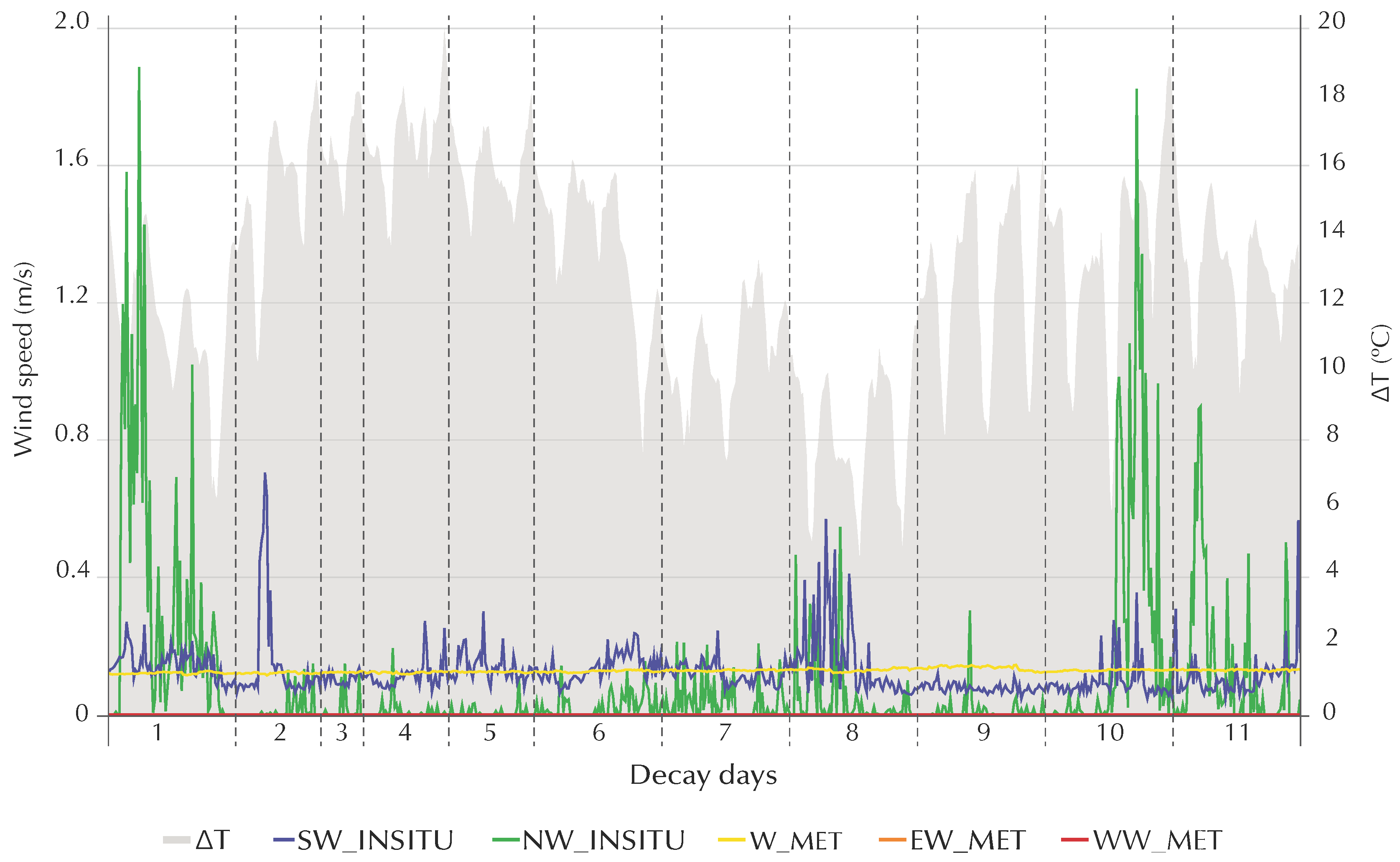
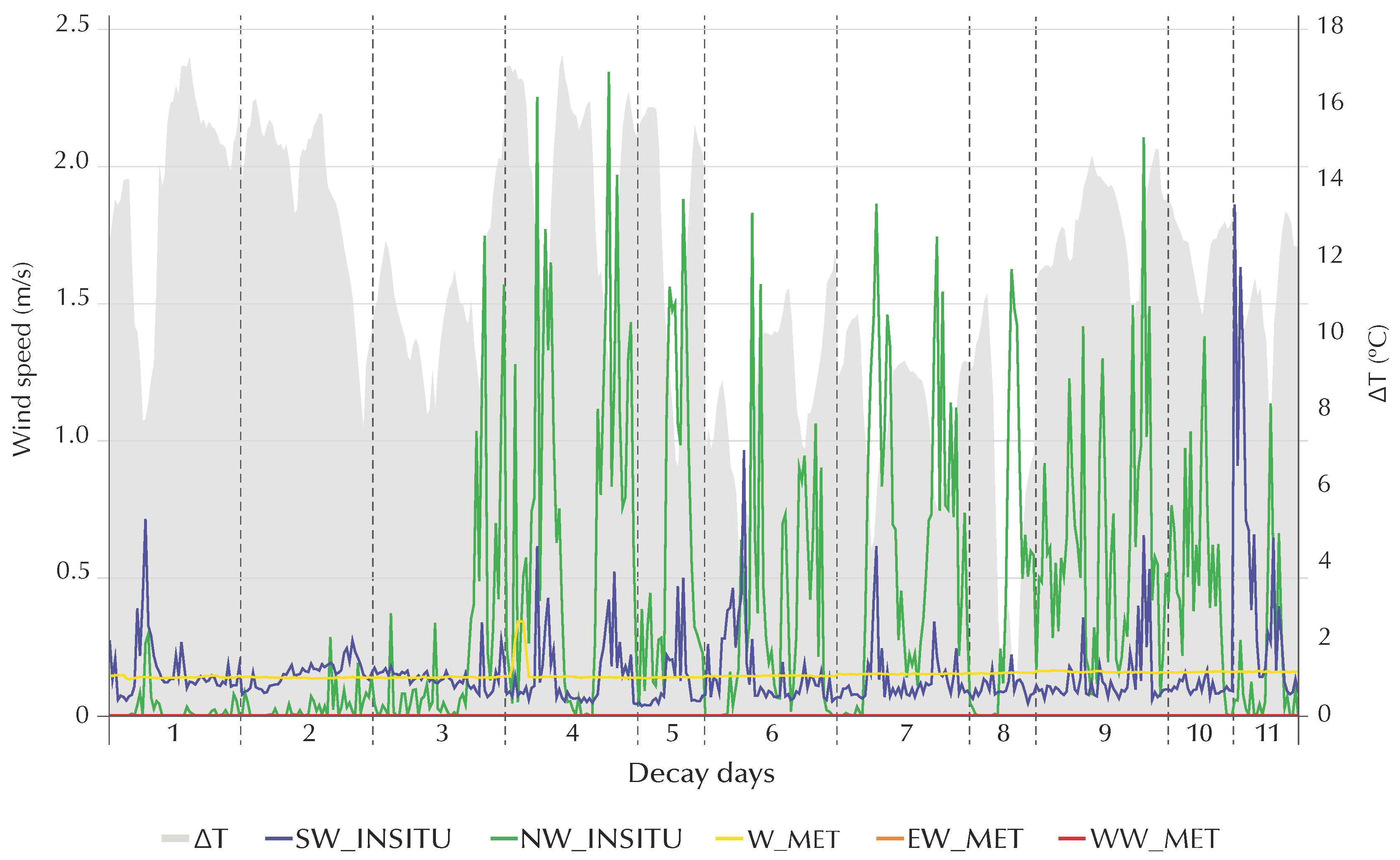
The precision of the weather conditions data is shown in

Table 1. Mean (µ) and standard deviation ($\sigma$) values of each measured data for each period.

Parameter	Index	P_1_T	P_2_C	P_3_C
CO${}_2$	µ (ppm)	613.75	561.14	629.78
	$\sigma$ (ppm)	316.80	378.57	278.47
$\Delta T$	µ (°C)	4.80	13.08	11.26
	$\sigma$ (°C)	10.29	3.17	3.85
W_MET	µ (m/s)	4.54	0.13	0.14
	$\sigma$ (m/s)	1.99	0	0
WW_MET	µ (m/s)	0.56	0	0
	$\sigma$ (m/s)	1.78	0	0
EW_MET	µ (m/s)	4.17	0.13	0.14
	$\sigma$ (m/s)	2.12	0	0
NW_INSITU	µ (m/s)	0.33	0.06	0.34
	$\sigma$ (m/s)	0.59	0.23	0.64
SW_INSITU	µ (m/s)	0.18	0.13	0.13
	$\sigma$ (m/s)	0.33	0.11	0.16

. P_1_T has 70% of the highest $\sigma$ values, which confirms it is a valuable period to train the models. Additionally, in this period, EW_MET has the highest dispersion of the data spread around the mean, mean = 4.17, and $\sigma$ = 2.12. On the other hand, the lowest one in the same period is SW_INSITU with a mean = 0.18, and $\sigma$ = 0.33, which means it is the most precise measurement. Figure 6, Figure 7 and Figure 8 demonstrate the wind speed and $\Delta T$ curves.

5.2. CO${}_2$ Uniformity

The tracer gas was homogeneous in the whole zone. We based the CO${}_2$ uniformity analysis on the method and requirements of ASTM E741 Standard for Air Change Measurements. This standard states that gas concentrations at representative locations throughout the zone should differ by less than 10% of the average concentration for the zone.

Table 2. Standard deviation ($\sigma$) values in % of each sensor from the average CO${}_2$ concentration.

Number	Model	$\mathsf{\sigma }$
1	OHM HD37VBTV.1	6.78
2	OHM HD37VBTV.1	4.87
3	CO210	4.98
4	CO210	9.15
5	CO210	6.52

shows the standard deviation ($\sigma$) in % of each sensor with respect to the mean value. This confirms that the calculations are according to the standard criteria.

5.3. Daily CO${}_2$ Measurements

Table 3. CO${}_2$ daily measurements at t = 0 in ppm. $C_{bg}$ means the daily average of the measured outdoor CO${}_2$ concentration in the air; $C_o$ is the average of the observed indoor CO${}_2$ concentration in the space, and $\sigma$ is the standard deviation of the day in ppm. Red is the highest value and green the lowest one.

Period	Days	${\mathit{C}}_{\mathbf{bg}}$	${\mathit{C}}_0$	$\mathsf{\sigma }$
P_1_T	1	379.19	1478.75	235.83
	2	390.02	1424.80	151.67
	3	378.06	3042.00	632.15
	4	380.58	1407.90	199.49
	5	394.63	1621.75	125.36
	6	382.85	1734.20	197.68
	7	389.84	2510.30	190.40
	8	394.37	1340.95	81.94
	9	389.67	2029.95	342.26
P_2_C	1	387.14	2001.00	384.65
	2	407.09	1992.00	429.72
	3	430.93	2010.00	326.85
	4	423.53	2002.2	389.57
	5	396.32	1996.80	390.57
	6	396.32	1831.20	300.96
	7	396.32	1898.40	344.78
	8	396.32	1509.00	260.68
	9	396.32	1798.80	343.96
	10	396.32	1898.40	389.03
	11	396.32	2002.20	396.81
P_3_C	1	393.89	1995.00	359.09
	2	435.66	1831.20	273.82
	3	408.42	1898.40	316.03
	4	377.11	1264.20	134.08
	5	381.34	1987.80	369.05
	6	385.24	1665.60	209.39
	7	386.35	1383.00	178.41
	8	399.52	1483.80	206.08
	9	373.74	1123.80	106.45
	10	371.24	1522.20	166.58
	11	384.37	1097.40	104.73

shows CO${}_2$ concentrations after injection, at the initial point t = 0. The color scale of the standard deviation is according to the values of each period. Although the correlation between the CO${}_2$ concentration and the wind is not linear, and infiltration also depends on the stack effect, it is possible to see some matching between them: When the SW_INSITU and WW_MET speeds are high, the standard deviation of that period is low, as happens in the second day of P_1_T and in the eleventh day of P_3_C. As illustrated in this table, the P_2_C has a high standard deviation on all days and a narrow range of $\sigma$ values. In contrast, the training period has a wide range of 81 ppm to 632 ppm of standard deviation, which is logical, because one of the main causes of air leakage is the wind speed, and the first nine days present more variable wind speed data than the other periods.

6. Results and Discussion

Before introducing the statistical indices proposed by ASTM D5157 for each of the fifteen combinations, it is important to look at the MBE values of the combinations. As shown in

Table 4. MBE values for each combination in P_1_T. The colors of the scale refer to each row, from the lowest (red) to the highest (green) values.

Model	Wind Speed Data
	W_MET	WW_MET	EW_MET	NW_INSITU	SW_INSITU
DFR	−58.42	0.56	−73.58	−69.20	−4.48
IFC	−65.44	−2.67	−65.43	−80.97	1.42
ELA	−58.99	1.14	−78.68	−81.88	−6.53

, the models with WW_MET and SW_INSITU present values very close to zero, having the lowest bias to represent the observed CO${}_2$ measurements: DFR with WW_MET, IFC with SW_INSITU, and ELA with WW_MET. On the other hand, the EP models with W_MET, EW_MET, and NW_INSITU data are the most inaccurate combinations, with the lowest MBE values, reaching as low as −81% underestimation, e.g., ELA with NW_INSITU. MBE was calculated only for P_1_T because the coefficients of the models were calculated for this period.

All results are presented in

Table 5. Results of the fifteen combinations according to ASTM D5157. The colors are the same as those defined in Figure 5. (Text in red color the values that do not meet the standard.)

Model	Wind	Period	$\overline{\mathit{C}}$${}_{\mathit{o}}$(ppm)	$\overline{\mathit{C}}$${}_{\mathit{p}}$(ppm)	R²	m	b	b/$\overline{\mathit{C}}$${}_{\mathit{o}}$ (%)	NMSE	FB	FS
DFR	W_MET	P_1_T	613.75	672.17	0.77	0.74	218.75	35.64	0.066	0.091	−0.335
		P_2_C	561.14	561.08	0.99	1.01	−4.11	−0.73	0.025	0.000	0.029
		P_3_C	629.78	633.54	0.93	1.06	−34.09	−5.41	0.017	0.006	0.095
	WW_MET	P_1_T	613.75	613.19	0.98	1.02	−14.32	−2.33	0.005	−0.001	0.062
		P_2_C	561.14	513.62	0.98	1.02	−58.20	−10.37	0.061	−0.088	0.053
		P_3_C	629.78	654.50	0.92	1.05	−5.58	−0.89	0.019	0.038	0.086
	EW_MET	P_1_T	613.75	689.16	0.71	0.71	254.43	41.45	0.083	0.116	−0.340
		P_2_C	561.14	453.47	0.97	1.01	−115.00	−20.49	0.237	−0.212	0.054
		P_3_C	629.78	608.74	0.93	1.08	−69.38	−11.02	0.021	−0.034	0.112
	NW_INSITU	P_1_T	613.75	682.95	0.73	0.71	249.37	40.63	0.077	0.107	−0.369
		P_2_C	561.14	546.98	0.99	1.02	−23.54	−4.19	0.026	−0.026	0.046
		P_3_C	629.78	667.60	0.99	1.02	−21.02	−3.34	0.021	0.058	0.076
	SW_INSITU	P_1_T	613.75	618.23	0.99	1.00	4.34	0.71	0.003	0.007	0.011
		P_2_C	561.14	478.58	0.99	1.03	−97.75	−17.42	0.034	−0.159	0.034
		P_3_C	629.78	617.04	0.99	1.03	−104.72	−16.63	0.014	−0.020	0.096
IFC	W_MET	P_1_T	613.75	679.19	0.68	0.73	230.51	37.56	0.087	0.101	−0.246
		P_2_C	561.14	402.32	0.96	1.00	−158.63	−28.27	0.533	-0.330	0.043
		P_3_C	629.78	625.57	0.93	1.07	−48.55	−7.71	0.019	-0.007	0.105
	WW_MET	P_1_T	613.75	616.42	0.97	1.05	−27.43	−4.47	0.011	0.004	0.130
		P_2_C	561.14	436.66	0.97	1.01	−130.01	−23.17	0.317	−0.250	0.052
		P_3_C	629.78	594.10	0.92	1.08	−86.08	−13.67	0.025	−0.058	0.118
	EW_MET	P_1_T	613.75	679.18	0.68	0.73	230.50	37.56	0.087	0.101	−0.246
		P_2_C	561.14	402.31	0.96	1.00	−158.63	−28.27	0.533	−0.330	0.043
		P_3_C	629.78	560.19	0.91	1.09	−128.74	−20.44	0.041	−0.117	0.136
	NW_INSITU	P_1_T	613.75	694.72	0.66	0.69	271.81	44.29	0.094	0.124	−0.333
		P_2_C	561.14	478.56	0.98	1.01	−90.21	−16.08	0.148	−0.159	0.051
		P_3_C	629.78	600.35	0.98	1.02	−103.60	−16.45	0.017	−0.048	0.092
	SW_INSITU	P_1_T	613.75	612.33	0.99	1.01	−9.64	−1.57	0.004	−0.002	0.041
		P_2_C	561.14	469.69	0.99	1.04	−82.75	−14.75	0.040	−0.177	0.037
		P_3_C	629.78	603.99	0.99	1.03	−111.95	−17.78	0.017	−0.042	0.097
ELA	W_MET	P_1_T	613.75	672.74	0.76	0.73	222.24	36.21	0.068	0.092	−0.336
		P_2_C	561.14	567.94	0.99	1.01	2.83	0.50	0.024	0.012	0.027
		P_3_C	629.78	642.73	0.92	1.05	−19.61	−3.11	0.019	0.020	0.092
	WW_MET	P_1_T	613.75	612.61	0.97	1.04	−25.45	−4.15	0.009	−0.002	0.107
		P_2_C	561.14	388.64	0.98	1.02	−112.34	−20.02	0.214	−0.202	0.058
		P_3_C	629.78	609.01	0.92	1.07	−65.59	−10.41	0.022	−0.034	0.110
	EW_MET	P_1_T	613.75	692.43	0.67	0.68	272.34	44.37	0.093	0.120	−0.353
		P_2_C	561.14	511.58	0.98	1.02	−59.28	−10.56	0.067	−0.092	0.052
		P_3_C	629.78	657.42	0.93	1.04	0.53	0.08	0.018	0.043	0.079
	NW_INSITU	P_1_T	613.75	695.63	0.68	0.69	270.87	44.13	0.091	0.125	−0.345
		P_2_C	561.14	508.33	0.98	1.02	−61.83	−11.02	0.073	−0.099	0.050
		P_3_C	629.78	624.93	0.99	1.02	−70.62	−11.21	0.015	−0.008	0.080
	SW_INSITU	P_1_T	613.75	620.28	0.99	0.98	19.65	3.20	0.004	0.011	−0.029
		P_2_C	561.14	498.13	0.99	1.03	−108.97	−19.42	0.020	−0.119	0.040
		P_3_C	629.78	623.77	0.99	1.04	−82.69	−13.13	0.014	−0.010	0.086

, followed by analysis and dispersion graphs, to facilitate a comparison between the three EnergyPlus models and the five wind inputs. As mentioned before, they were evaluated according to the criteria of the ASTM D5157 Standard, which requires compliance in all periods.

The SW_INSITU with the three infiltration models is the wind data that delivers the best results in all periods. This was expected because these data refer to the wind that impinges directly on the main façade of the test room. The WW_MET was used as the second wind data, and it performs the best in the three seasons and with the three models. These two wind data that meet the ASTM D5157 criteria are related to the room orientations, southeast and southwest, which could be the reason for their good agreement. In Appendix D, it can be seen that these combinations are the only ones that present a quadratic relation of the wind (values of D coefficient), which also could be the reason why these data resulted in the best CO${}_2$ prediction. Although P_1_T presents a lower standard deviation (316.80 ppm) of CO${}_2$ than P_2_C (378.57 ppm), EP models with SW_INSITU and WW_MET are still capable of predicting the measured CO${}_2$ concentration.

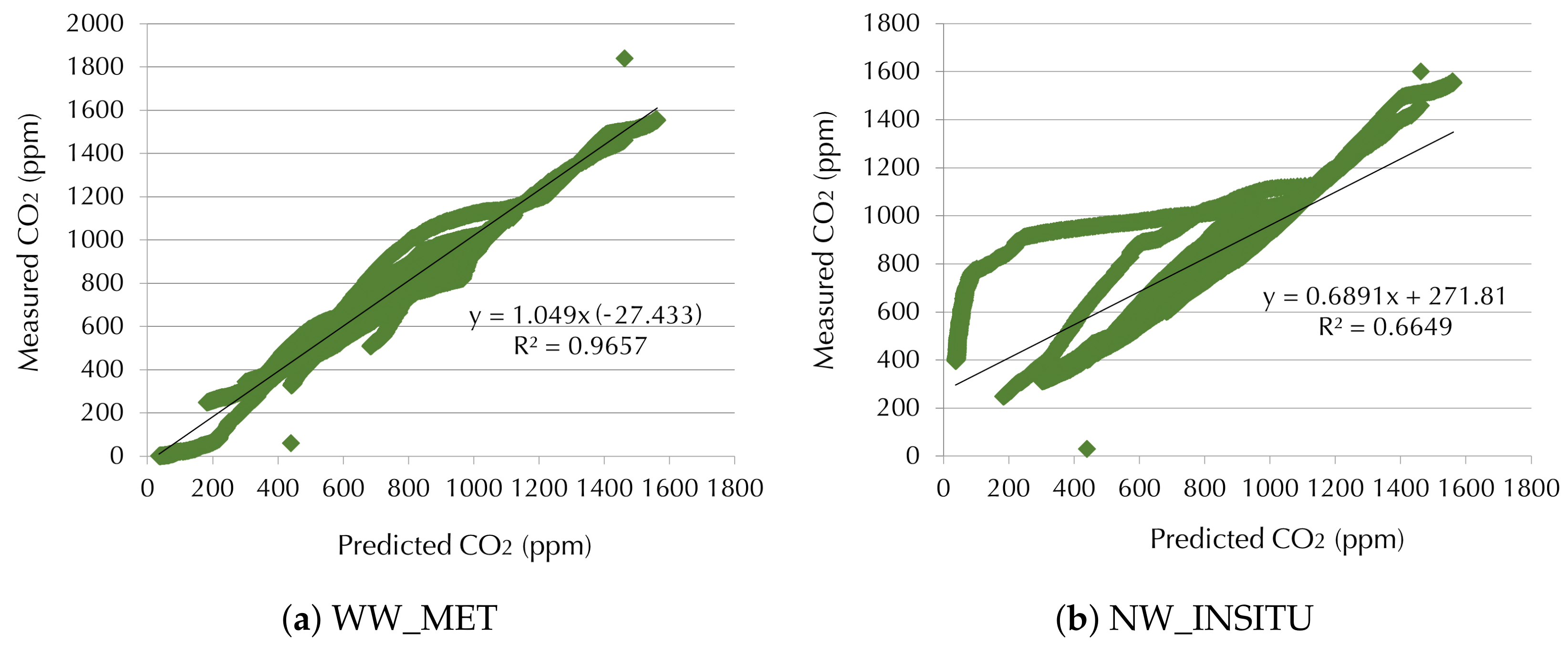
On the other hand, W_MET, EW_MET, and NW_INSITU do not approve the standard requirements in P_1_T with any air leakage object, presenting values of R² from 23% to 29%, worse than SW_INSITU in the same period. As aforementioned, these wind data are also the most inaccurate ones. The data variability of P_1_T requires the right wind data to produce high-quality models. Dispersion graphs in Figure 9 show the good and the bad correlation between the predicted and measured CO${}_2$ concentration in the first period provided by DFR using SW_INSITU and EW_MET, respectively.

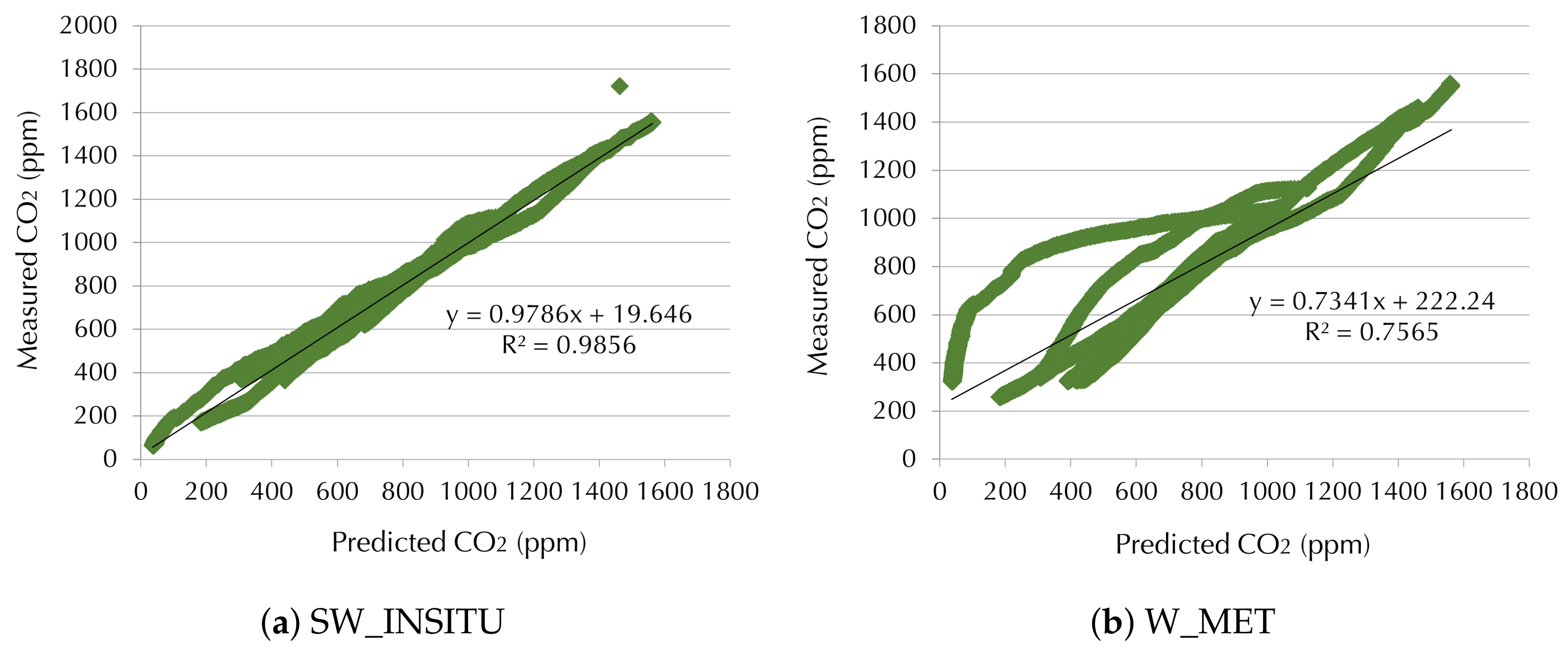
Similar results are found when combining the IFC and ELA objects with the five wind data. W_MET, EW_MET, and NW_INSITU again do not meet the ASTM D5157 criteria, as many parameters such as R², m, and b/$\overline{C}$${}_o$(%) were outside the requirements in P_1_T. Furthermore, in P_2_C the IFC model with the wind data from the weather station (W_MET, EW_MET, and WW_MET) have NMSE values higher than those demanded by the standard. Despite this, IFC with WW_MET has the best NMSE value with a difference of 21% with respect to the limit (0.25), while the others have more than twice the difference. Dispersion graphs in Figure 10 and Figure 11 clearly illustrate the distinction between the best combination (IFC with WW_MET and ELA with SW_INSITU), and the worst (IFC with NW_INSITU, and ELA with W_MET).

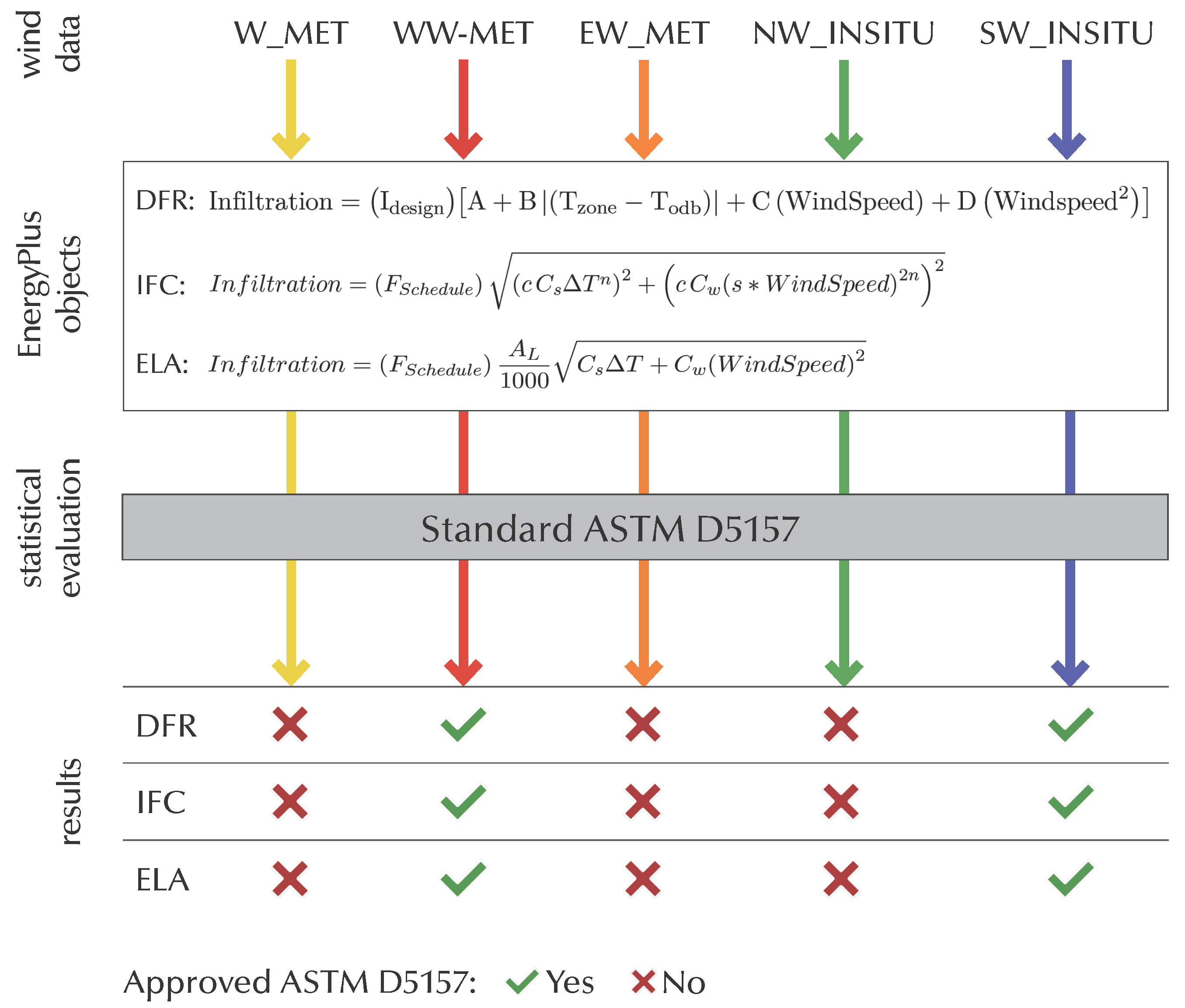
In summary, the wind data W_MET, EW_MET, and NW_INSITU are inadequate to represent the actual infiltration of this case study. This is especially noteworthy in the case of W_MET because it is the global wind used by any BEM software and many energy modellers. There is useful information inside W_MET, but when applied without wind disaggregation, it produces a misleading effect. This raises doubts about the direct use of this type of wind in energy estimations and calibration of energy models without wind disaggregation. Therefore, for this study, the WW_MET ASTM D5157 approval in the training period represents an alternative and cost-effective option to select the best wind data to calculate air leakage, in case it is not possible to install in situ sensors. Figure 12 summarises the results of this research.

It is noteworthy that in this study, we did not analyse whether the wind data and the infiltration model were wrong or right. We only highlighted that since our main purpose was to calibrate building energy models, we needed real-time wind data; otherwise, the infiltration values would not be accurate in high-time estimations. On the other hand, for annual energy simulations, the application of the TMY format might be suitable.

7. Conclusions

In this paper, the application of the wind data from a weather file (herein as global wind) to estimate the infiltration of a test space was evaluated. To calculate air leakage, three infiltration models of EnergyPlus with algebraic equations were used: DesignFlowRate (DFR), FlowCoefficient (IFC), and EffectiveLeakageArea (ELA). These models were applied with four other wind data: from the weather file, eastbound and westbound wind data were used, as well as the wind data from in situ sensors (on southeast and northwest façades), to understand which combination delivered the best result. All fifteen combinations were empirically evaluated according to an experiment of CO${}_2$ concentration decay carried out in a test room. The empirical validation of the results was carried out taking into account the requirements of ASTM D5157 to evaluate IAQ in three periods: The summer data were used as training, and winter and spring data were used for validation.

As far as the authors know, the empirical comparison of different wind data with EnergyPlus infiltration models, as well as the application of ASTM D5157 to assess these models, have never been carried out before. The results are specific to this test room and the main conclusions are as follows:

• The best combinations and the only ones that meet the ASTM D5157 criteria use the wind speed measured in situ on the southeast façade and the west wind from the weather file. Both wind data are related to the unsealed orientations of the test space.
• The use of the global wind from the weather file is not the most accurate option to estimate infiltration with any EP model. This raises doubts about the use of this wind in the calibration of energy models without wind disaggregation.
• Global wind disaggregation is a good and cost-effective strategy to apply with EnergyPlus air leakage models and results in accurate infiltration values.

Further research should be carried out to verify whether these results occur in other rooms of the same apartment, and other buildings as well. In addition, the application of disaggregated wind data should be implemented in the calibration process of BEMs, by using a schedule activation in EnergyPlus to accurately account for infiltration and achieve better energy predictions. As a recommendation, EnergyPlus should take wind direction into account in air leakage estimates, just as it does in calculating façade convection coefficients.

References

1. Bekker, S. The EU’s recovery and resilience facility: A next phase in EU socioeconomic governance? Politics Gov. 2021, 9, 175–185. [Google Scholar] [CrossRef]
2. Unión Europea Reglamento (UE) 2021/241 del Parlamento Europeo y del Consejo de 12 de febrero de 2021 por el que se establece el Mecanismo de Recuperación y Resiliencia. Diario Oficial de la Unión Europea, 30 September 2010; 1–59.
3. De la Porte, C.; Jensen, M.D. The next generation EU: An analysis of the dimensions of conflict behind the deal. Soc. Policy Adm. 2021, 55, 388–402. [Google Scholar] [CrossRef]
4. Bastos Porsani, G.; Del Valle de Lersundi, K.; Sánchez-Ostiz Gutiérrez, A.; Fernández Bandera, C. Interoperability between Building Information Modelling (BIM) and Building Energy Model (BEM). Appl. Sci. 2021, 11, 2167. [Google Scholar] [CrossRef]
5. Ruiz, G.R.; Bandera, C.F.; Temes, T.G.A.; Gutierrez, A.S.O. Genetic algorithm for building envelope calibration. Appl. Energy 2016, 168, 691–705. [Google Scholar] [CrossRef]
6. Fernández Bandera, C.; Ramos Ruiz, G. Towards a new generation of building envelope calibration. Energies 2017, 10, 2102. [Google Scholar] [CrossRef]
7. Manfren, M.; Aste, N.; Moshksar, R. Calibration and uncertainty analysis for computer models–a meta-model based approach for integrated building energy simulation. Appl. Energy 2013, 103, 627–641. [Google Scholar] [CrossRef]
8. The American Society of Heating, Refrigerating and Air-Conditioning Engineers. The 2017 ASHRAE Handbook—Fundamentals; ASHRAE: Peachtree Corners, GA, USA, 2017. [Google Scholar]
9. Du, H.; Jones, P.; Segarra, E.L.; Bandera, C.F. Development of a REST API for obtaining site-specific historical and near-future weather data in EPW format. In Proceedings of the 4th IBPSA-England Conference on Building Simulation and Optimization, Cambridge, UK., 11–12 September 2018. [Google Scholar]
10. Bhandari, M.; Shrestha, S.; New, J. Evaluation of weather datasets for building energy simulation. Energy Build. 2012, 49, 109–118. [Google Scholar] [CrossRef]
11. Segarra, E.L.; Ruiz, G.R.; González, V.G.; Peppas, A.; Bandera, C.F. Impact Assessment for Building Energy Models Using Observed vs. Third-Party Weather Data Sets. Sustainability 2020, 12, 6788. [Google Scholar] [CrossRef]
12. Gutiérrez, V.; Ramos Ruiz, G.; Fernández Bandera, C. Impact of Actual Weather Datasets for Calibrating White-Box Building Energy Models Base on Monitored Data. Energies 2021, 14, 1187. [Google Scholar] [CrossRef]
13. González, V.G.; Ruiz, G.R.; Segarra, E.L.; Gordillo, G.C.; Bandera, C.F. Characterization of Building Foundation in Building Energy Models. In Proceedings of the Building Simulation, Rome, Italy, 2–4 September 2019. [Google Scholar]
14. Lee, S.H.; Hong, T. Validation of an inverse model of zone air heat balance. Build. Environ. 2019, 161, 106232. [Google Scholar] [CrossRef]
15. Hong, T.; Lee, S.H. Integrating physics-based models with sensor data: An inverse modeling approach. Build. Environ. 2019, 154, 23–31. [Google Scholar] [CrossRef]
16. Taddeo, P.; Ortiz, J.; Salom, J.; Segarra, E.L.; González, V.G.; Ruiz, G.R.; Bandera, C.F. Comparison of experimental methodologies to estimate the air infiltration rate in a residential case study for calibration purposes. In Proceedings of the 39th AIVC 2018-Smart Ventilation for Buildings, Antibes Juan-Les-Pins, France, 18–19 September 2018; p. 68. [Google Scholar]
17. Han, G.; Srebric, J.; Enache-Pommer, E. Different modeling strategies of infiltration rates for an office building to improve accuracy of building energy simulations. Energy Build. 2015, 86, 288–295. [Google Scholar] [CrossRef]
18. Davenport, A.; Hui, H. External and Internal Wind Pressures on Buildings; BLWT820133; Boundary Layer Wind Tunnel Laboratory, University of Western Ontario: London, ON, Canada, 1982. [Google Scholar]
19. Raman, G.; Chelliah, K.; Prakash, M.; Muehleisen, R.T. Detection and quantification of building air infiltration using remote acoustic methods. In INTER-NOISE and NOISE-CON Congress and Conference Proceedings; Institute of Noise Control Engineering: Washington, DC, USA, 2014; Volume 249, pp. 3976–3985. [Google Scholar]
20. Persily, A.K.; Emmerich, S.J. Energy Impacts of Infiltration and Ventilation in US Office Buildings Using Multizone Airflow Simulation. Proc. Iaq Energy 1999, 98, 191–206. [Google Scholar]
21. Miszczuk, A.; Heim, D. Parametric study of air infiltration in residential buildings—The effect of local conditions on energy demand. Energies 2021, 14, 127. [Google Scholar] [CrossRef]
22. Jokisalo, J.; Kurnitski, J.; Korpi, M.; Kalamees, T.; Vinha, J. Building leakage, infiltration, and energy performance analyses for Finnish detached houses. Build. Environ. 2009, 44, 377–387. [Google Scholar] [CrossRef]
23. Wilkki, C.M.; Reeve, N. Communication from the Commission to the European Parliament, the Council, the European Economic and Social Committee and the Committee of the Regions on European Missions European Commission Directorate-General for Research and Innovation Directorate G—Common Policy Centre; European Commission: Brussels, Belgium, 2021. [Google Scholar]
24. DoE. EnergyPlus Engineering Reference: The Reference to EnergyPlus Calculations; Lawrence Berkeley National Laboratory: Berkeley, CA, USA, 2021.
25. Ng, L.C.; Quiles, N.O.; Dols, W.S.; Emmerich, S.J. Weather correlations to calculate infiltration rates for US commercial building energy models. Build. Environ. 2018, 127, 47–57. [Google Scholar] [CrossRef]
26. Dols, W.S.; Emmerich, S.J.; Polidoro, B.J. Coupling the multizone airflow and contaminant transport software CONTAM with EnergyPlus using co-simulation. Build. Simul. 2016, 9, 469–479. [Google Scholar] [CrossRef]
27. Ng, L.C.; Dols, W.S.; Emmerich, S.J. Evaluating potential benefits of air barriers in commercial buildings using NIST infiltration correlations in EnergyPlus. Build. Environ. 2021, 196, 107783. [Google Scholar] [CrossRef]
28. Shrestha, S.; Hun, D.; Moss, C. Modeling Whole Building Air Leakage and Validation of Simulation Results against Field Measurements. In Whole Building Air Leakage: Testing and Building Performance Impacts; ASTM International: West Conshohocken, PA, USA, 2019. [Google Scholar]
29. Bae, Y.; Joe, J.; Lee, S.; Im, P.; Ng, L. Evaluation of Existing Infiltration Models Used in Building Energy Simulation. Technical report; Oak Ridge National Lab (ORNL): Oak Ridge, TN, USA, 2021. [Google Scholar]
30. Winkler, J.M.; Horowitz, S.G.; DeGraw, J.W.; Merket, N.D. Evaluating EnergyPlus Airflow Network Model for Residential Ducts, Infiltration, and Interzonal Airflow; Technical report; National Renewable Energy Lab (NREL): Golden, CO, USA, 2017.
31. BEopt: Building Energy Optimization Tool. Available online: https://www.nrel.gov/buildings/beopt.html (accessed on 2 December 2022).
32. ASTM E741-11; Standard Test Method for Determining Air Change in a Single Zone by Means of a Tracer Gas Dilution. American Society for Testing and Materials: West Conshohocken, PA, USA, 2017.
33. Sherman, M.H. Tracer-gas techniques for measuring ventilation in a single zone. Build. Environ. 1990, 25, 365–374. [Google Scholar] [CrossRef]
34. Sherman, M. Uncertainty in air flow calculations using tracer gas measurements. Build. Environ. 1989, 24, 347–354. [Google Scholar] [CrossRef]
35. Sherman, M. On the estimation of multizone ventilation rates from tracer gas measurements. Build. Environ. 1989, 24, 355–362. [Google Scholar] [CrossRef]
36. Chao, C.Y.; Wan, M.; Law, A.K. Ventilation performance measurement using constant concentration dosing strategy. Build. Environ. 2004, 39, 1277–1288. [Google Scholar] [CrossRef]
37. Cui, S.; Cohen, M.; Stabat, P.; Marchio, D. CO2 tracer gas concentration decay method for measuring air change rate. Build. Environ. 2015, 84, 162–169. [Google Scholar] [CrossRef]
38. Gowri, K.; Winiarski, D.W.; Jarnagin, R.E. Infiltration Modeling Guidelines for Commercial Building Energy Analysis; Technical report; Pacific Northwest National Lab (PNNL): Richland, WA, USA, 2009.
39. Hunt, C. Air infiltration: A review of some existing measurement techniques and data. In Building Air Change Rate and Infiltration Measurements; American Society for Testing and Materials: West Conshohocken, PA, USA, 1980. [Google Scholar]
40. Duda, S. Common Evaluation Metrics for Regression Analysis. 2021. Available online: https://scottmduda.medium.com/common-evaluation-metrics-for-regression-analysis-4b62726f1aad (accessed on 2 December 2022).
41. ASTM D5157-19; Standard Guide for Statistical Evaluation of Indoor Air Quality Models. American Society for Testing and Materials: West Conshohocken, PA, USA, 2019.
42. Ng, L.C.; Persily, A.K.; Emmerich, S.J. Improving infiltration modeling in commercial building energy models. Energy Build. 2015, 88, 316–323. [Google Scholar] [CrossRef]
43. Remion, G.; Moujalled, B.; El Mankibi, M. Review of tracer gas-based methods for the characterization of natural ventilation performance: Comparative analysis of their accuracy. Build. Environ. 2019, 160, 106180. [Google Scholar] [CrossRef]
44. The American Society of Heating, Refrigerating and Air-Conditioning Engineers. Handbook; ASHRAE: Peachtree Corners, GA, USA, 2017. [Google Scholar]
45. Emmerich, S.; Howard-Reed, C.; Nabinger, S. Validation of multizone IAQ model predictions for tracer gas in a townhouse. Build. Serv. Eng. Res. Technol. 2004, 25, 305–316. [Google Scholar] [CrossRef]
46. E.V.O. Uncertainty Assessment for IPMVP; E.V.O.: Washington, DC, USA, 2018; pp. 1–82. [Google Scholar]
47. Achenbach, P.R.; Coblenz, C. Field measurements of air infiltration in ten electrically heated houses. Ashrae Trans. 1963, 69, 358–365. [Google Scholar]
48. Walker, I.S.; Wilson, D.J. Field validation of algebraic equations for stack and wind driven air infiltration calculations. HVAC&R Res. 1998, 4, 119–139. [Google Scholar]
49. ASTM E779-19; Standard Test Method for Determining Air Leakage Rate by Fan Pressurization. American Society for Testing and Materials: West Conshohocken, PA, USA, 2019.
50. Sherman, M.H. Infiltration-Pressurization Correlation: Simplified Physical Modeling; Lawrence Berkeley National Laboratory: Berkeley, CA, USA, 1980.
Figure 1. External view of the apartment is indicated in yellow.
Buildings 13 00511 g001
Figure 2. Isometric representation of the five openings of the room. The panels in two interior wooden doors are divided into two parts: The first is glazed with wooden mullions, and the lower part is only made of wood. The main door (D1) is 1.72 m², and the secondary door (D2) is 1.61 m². The southwest façade has a tilt-and-turn window (W1) (2.47 m²), the southeast façade has a door window (W2) with an area of 4.66 m², and a tilt-and-turn window (W3) with an area of 1.79 m². All windows are made of aluminium, double-clear glass of 3 mm each, and an air cavity of 13 mm. See Figure 3 for the plan view.
Buildings 13 00511 g002
Figure 3. Plan of the apartment. W, window; D, door. Numbers are CO 2 sensors. Sensor 1 was installed at 0.40 m above the ground; sensor 2 at 0.74 m; sensor 3 at 1.19 m; sensor 4 at 0.74 m, and sensor 5 at 1.52 m.
Buildings 13 00511 g003
Figure 4. Northeast side view of the room. D, door; numbers are CO 2 sensors.
Buildings 13 00511 g004
Figure 5. Graphical representation of selected wind speed data. W_MET is the weather station winds (herein as global wind) from 0° to 360°; WW_MET and EW_MET are the weather station west and east winds from 181° to 360° and 0° to 180°, respectively; NW_INSITU is the wind data recorded by the wind speed sensor on the northwest terrace; SW_INSITU is the wind data collected on the southeast terrace.
Buildings 13 00511 g005
Figure 6. Wind speed and Δ T averages of summer (P_1_T) at ten-minute time-step. This period presents higher wind and Δ T variability, especially in the weather station’s wind data, according to which the wind speed sometimes exceeds 10 m/s.
Buildings 13 00511 g006
Figure 7. Wind speed and Δ T averages of winter (P_2_C) at ten-minute time-step. Most days have practically the same wind rhythm pattern. In contrast to P_1_T, the weather station data are equal to zero or maintain the same value almost every day. In this figure, it is difficult to see the EW_MET because its curve is behind the W_MET.
Buildings 13 00511 g007
Figure 8. Wind speed and Δ T averages of spring (P_3_C) at ten-minute time-step. As in the second period, there is a rise and fall pattern, which is more evident for W_MET and WW_MET. In this figure, it is difficult to see the EW_MET because its curve is behind the W_MET.
Buildings 13 00511 g008
Figure 9. Correlation between predicted and measured CO 2 concentration by DFR models with SW_INSITU (a) and EW_MET (b) in P_1_T.
Buildings 13 00511 g009
Figure 10. Correlation between predicted and measured CO 2 concentration by IFC models with WW_MET and NW_INSITU in P_1_T.
Buildings 13 00511 g010
Figure 11. Correlation between predicted and measured CO 2 concentration by ELA models with SW_INSITU and W_MET in P_1_T.
Buildings 13 00511 g011
Figure 12. Summary of the paper results.
Buildings 13 00511 g012