1. Introduction
Curved beams are important constituents of many engineering and aerospace structures, and they have been applied in various components, such as high-speed machinery, vehicle shells, and lightweight bridges. The curved bridge has a unique streamlined structure, with smooth and bright lines, designed so that the structure and the surrounding environment are in harmony, in line with the public’s aesthetic needs. Such bridges are more suitable than straight beams in mountainous areas [
1] (Yao Lingsen,1989). Curved girders play an important role in urban bridges and highways [
2] (Zhao, Y.Y. et al., 2006), and curved girder bridges can be a good solution to problems such as topography and constraints imposed by tall buildings. However, when constrained by factors such as small spaces in urban construction, bridges with different radii of curvature must be arranged together, usually with a bridge of variable curvature as a transition between them. These bridges can be similarly used between curved and straight segments [
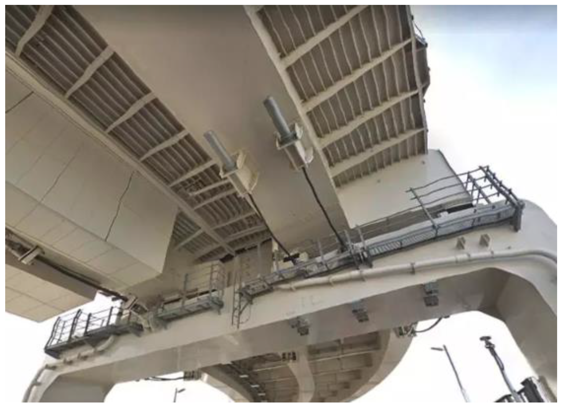
3] (Zhang Yuanhai, 2005). As shown in
Figure 1 and
Figure 2, curved bridges are used in a wide range of applications, either as viaducts between cities or across mountains, valleys, and seas.
When a vehicle moves on a variable-curvature girder bridge, unlike a straight girder segment, in addition to the vertical moving load, a torsional moment related to the radius of curvature is generated on the girder, which means the dynamic response is more complex [
4]. Therefore, studying the dynamic response of variable curvature girders can prevent lateral overturning and fatigue damage to the girders. As shown in
Figure 3, when considering the dynamic response of a bridge affected by vehicle loads, the steel box beam is generally taken as the main bearing member. Hence, it is necessary to study elliptical curved steel beams. The mechanical model designed in this study is a simplified form of an actual bridge.
Theoretical and experimental studies on curved girder bridges have been conducted since the early 1980s, with fruitful results. Vlasov et al. [
5] studied the curved-beam structure with a circular cross-section and proposed the statics theory of elastic thin-walled members. Morri D.L. et al. [
6] used the finite element method to study curved-beam structures. Based on the basic equation of a curved beam, Ni Guorong, Wang Yong, and Xiong Guoxiang [
7] used differential equations and numerical integration involving parabolic, hyperbolic, elliptical, and variable-curvature beams to find engineering solutions for beams with variable cross-sections and curvatures. In recent years, many research institutes have also achieved success in the field of variable curvature beams. C. Yu et al. [
8] conducted a dynamic sensitivity analysis based on a variable-curvature beam model with functionally graded porous FGP under general boundary conditions. Qingshan Wang et al. [
9] studied the convergence and numerical verification of laminated composite beams with variable curvature under different boundary conditions. Jie Yu [
10] derived an analytical solution to the static force of a beam with variable curvature. Mingdong Chen derived the stiffness matrix of a beam of constant curvature [
11].
The calculation of the dynamic response of a bridge under a moving load is the basic problem of vehicle–bridge coupling, which was solved in terms of mechanics principles [
12]. At present, the dynamics of curved beams is still a multi-scale and diversified research direction. Jun Luo et al. [
13] proposed a semi-analytical solution for the free vibration of curvilinear rails with a vehicle–bridge coupling. Abdoos H. et al. [
14] achieved the out-of-plane dynamic response of a curved beam under the action of a moving mass underlying an elastic foundation. S. H. Li et al. [
15] obtained analytical solutions for the vertical, torsional, radial, and axial responses of a curved beam under a three-way moving load. Poojary Jatin et al. [
16] developed a cracked bending beam element to investigate the effects of moving load velocity, depth, and crack location on the dynamic response of the beam in combination with the presence of cracks in the structure. Fei Han et al. [
17] explored the coupling effect of vehicle speed on vehicle driving dynamic response under a random vehicle load. Xia Zhang et al. [
18] integrated the influences of various factors on the dynamic response of a curved deck.
The precise integration method pioneered by Wanxie Zhong [
19] can still obtain a highly accurate numerical solution to the problem where the applied point of the external dynamic load is fixed, i.e., using a sizable integral time step. Y.B. Yang and C.M. Wu [
20] derived analytical solutions for horizontal curved beams under vertical and horizontal moving loads, providing clear physical insights into various vehicle-induced phenomena on curved beams. Jong-Shyong Wu and Lieh-Kwang Chiang [
21] obtained the stiffness and mass matrices of a curved-beam element from the force–displacement relationship and kinetic energy equation by considering the effects of out-of-plane shear deformation of the curved beam and the effects of rotational inertia due to bending and torsional vibrations. They obtained the dynamic response under moving loads at different radii of curvature. Yahui Zhang [
22] constructed the right-end term of the dynamic equation that can simulate the continuous movement of loads. A precise integral 2N algorithm was used to solve the dynamic equation. The dynamic response of a uniform, simply supported straight beam under a moving load was solved. Typical numerical calculations showed that the obtained numerical solution was almost identical to the analytical solution, even when using a sparse mesh division. In the case of the external load acting on the structure being strictly linear within the integral step, the high-precision structural-response time history could be obtained, even when the integral step was more extensive. Hence, the algorithm has been widely used in the dynamic structural analysis of straight girder bridges, optimal control, precise solutions of partial differential equations, and unsteady stochastic dynamics. Junping Pu et al. [
23] applied the precise integration method to simulate the dynamic response processes of isotropic and variable-section simply supported girder bridge models under moving simple harmonic loads. Q. Gao et al. [
24] proposed a fast and accurate integration method for solving structural dynamics problems. Yuefeng Shao et al. [
25] proposed an algorithm for vehicle–bridge coupling and sensitivity analysis based on the step-by-step solution technique of the exact time integral method. The dynamic response of a discrete-supported curved track under moving loads with different curvatures, speeds, and other influencing factors was analyzed by Chen-Chen Zheng and Qiang Huang et al. [
26]. The effects of uncertain parameters and random ground shaking on the seismic response and dynamic damage probability of slopes were analyzed and discussed by Rui Pang et al. [
27]. Tomasz Maleska and Damian Beben [
28] presented the results of a numerical study of earth-steel bridges with different overburden depths under seismic excitation and analyzed the results of different boundary conditions for earth-steel bridges with the same soil overburden depth. Xiaofei Li and Haosen Zhai et al. [
29] constructed the stiffness matrices of curved beams using a semi-analytical method of structural mechanics.
The finite element method has been one of the most common methods recently used to study the subject of curved beams, but much work has been involved when building different models. For example, finite element modeling is limited by the variation of curvature when studying curved beams with variable curvature, and it is impractical to use the sparse cell division method for curved beams with large curvature; otherwise, it will cause large errors. In this study, we propose a model based on structural mechanics, which can obtain efficient and accurate numerical calculation results using the precise integration method. In this study, the dynamic theory of structural out-of-plane variable curvature beams is analyzed based on existing studies. We take the dynamic response of a variable-curvature beam under a vehicle load as the research object; this can contribute to the subsequent engineering analysis of dangerous sections under vehicle loads and the prevention of bridge damage. In addition to moving loads, when considering the influence of external dynamic loads on steel structures with variable curvature, the precise integration method can be applied to simulate the steel structure, which can obtain more accurate dynamic time-course results more efficiently, to prevent damage to the steel beam with variable curvature, control the beam vibration, etc.
2. Basic Principles of Precise Integration
The method of fine integration is essentially a high-precision method for calculating partial differential equations, which uses the basic principle of multi-scale wavelet transform to construct a multi-scale wavelet interpolation operator. It then uses the operator to discretize the partial differential equation into a system of ordinary differential equations. Finally, the system of equations is solved by the fine integration method.
The multi-degree-of-freedom dynamic balance equation in structural dynamics is
where
M,
C, and
K are the mass, damping, and stiffness matrices, respectively;
,
, and
are the displacement, velocity, and acceleration vectors, respectively, of the structure; and
F(t) is the external force vector.
If the initial displacement
and initial velocity
are known, the intermediate variable
p can be set so that
, i.e.,
, and we can obtain
For convenience, let
where
,
,
, and
.
In practical problems, the mass, damping, and stiffness of the structure are all known parameters, so the matrix
H is also a constant moment. Substituting Equations (3)–(5) into Equation (2), we can write the inhomogeneous equation,
i.e., the structural dynamics response equation, for which the general solution is
We introduce the exponential matrix
for which the precise solution is obtained by reducing it to
where
m can be chosen as
; since
, which itself is not a large time interval,
will be a much smaller time interval. For the time interval
, we apply a Taylor expansion to obtain
where
I is the unit matrix and
, where
L denotes the truncated phase of the Taylor expansion. Substituting Equation (10) into Equation (9), we obtain
By the recurrence law of 2N, , where the middle term in the recurrence relation is .
Thus, Equation (11) can be written as
Generally, the calculation of is sufficiently accurate and satisfies the requirements if we take L = 4 and N = 20.
For the homogeneous equation, the integral term of the general solution of the dynamic response equation is zero. For the time-invariant system,
H is a constant matrix. The general solution of the equation takes the following form:
Let the time step delta equal
τ. Then,
After the matrix
T is calculated by the above method, the time integration becomes
For non-homogeneous equations, if the non-homogeneous term
r is linear in the time step
, i.e., the equation is
then we can formulate
3. Variable-Curvature Beam Analysis
Based on the precise integration method, a known matrix H is a prerequisite for the analysis of the dynamic response of a curved beam with variable curvature under moving loads. This means that the discrete method is used to divide the beam into segments and find the stiffness matrix K, mass matrix M, and damping matrix C under the parameters of the model.
The definition of a variable-curvature beam is that the curvature of each point on the beam is different, which means that the solution of the geometric relationship of the linear term is the premise of analyzing the subsequent dynamics problems. There are various types of lines with variable curvatures, such as sinusoids, catenaries, ellipses, and so on. In addition, the line shape also needs to consider whether the curvature changes quickly or slowly; i.e., different bending beam models can be obtained by changing different line shape parameters and can be compared against the constant curvature model. In summary, elliptic curve beams that meet all the above requirements are the main objects of this study.
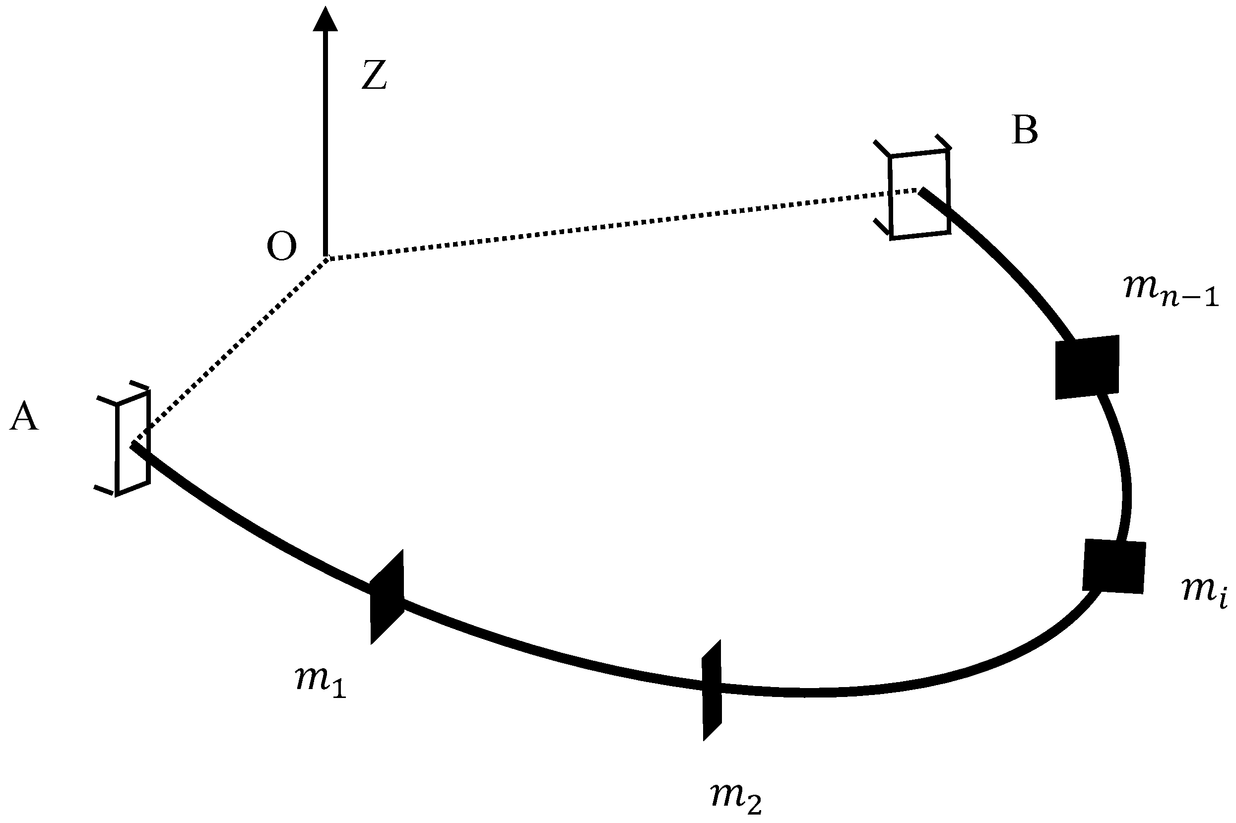
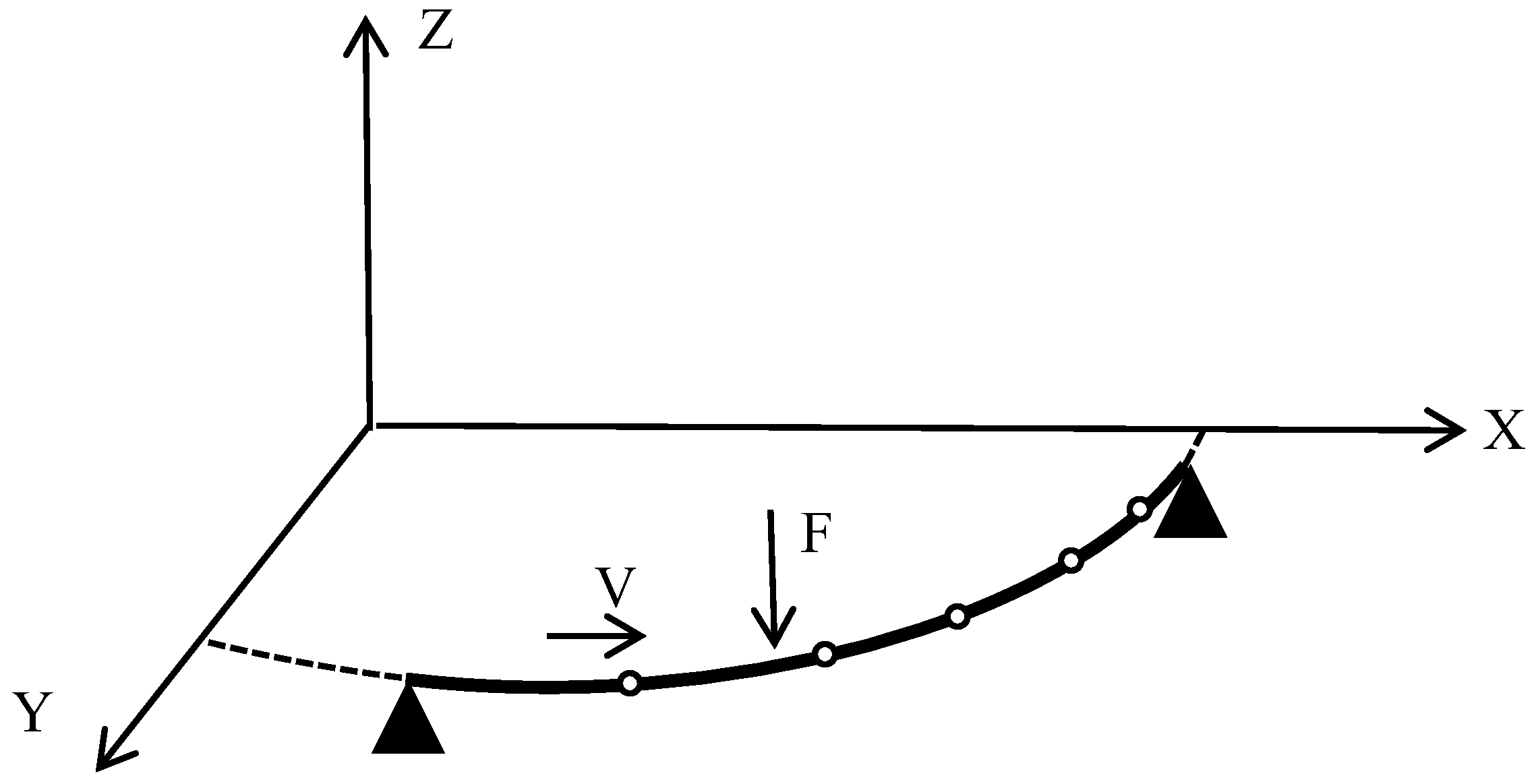
Owing to the structural form of a space-curved beam, it is appropriate to use a column coordinate system to analyze the problem. The out-of-plane curved beam is divided into
N segments. Hence, there are
N + 1 nodes, each with three degrees of freedom, i.e., vertical, radial around the plane, and tangential rotation around the plane, corresponding to three forms of out-of-plane generalized loads, i.e., vertical force
, radial force couple
, and circumferential torque
, as shown in
Figure 4.
Only three internal forces are generated in any section of the full beam: shear force perpendicular to the plane of the curved beam, bending moment around the radial axis, and torque around the circumferential axis. The restraint at the end section of the beam requires that these three reaction forces be provided to the extent that no rigid body displacement occurs in the full beam. Therefore, the three forms of reaction forces provided by the constraint at boundary A are vertical force , force dipole moment , and torque . As a result, in this study, the variable curvature beam is set as a cubic super-stationary structure.
Excluding the fixed ends of the beam, the number of nodes is N − 1, and each node has three degrees of freedom: vertical, rotational, and torsional. Therefore, the dimension of the stiffness matrix is 3(N − 1) 3(N − 1), and similarly for the flexibility matrix. The stiffness matrix can be obtained by inverting the flexibility matrix. The elements in any column of the flexibility matrix D represent the displacements of the remaining nodes under a unit load. In this way, the entire flexibility matrix can be decomposed into a superposition of nine flexibility matrices: vertical uncoupled, rotational uncoupled, torsional uncoupled, vertical-torsional coupled, vertical-torsional coupled, rotational-vertical coupled, rotational-torsional coupled, torsional-vertical coupled, and torsional-torsional coupled. These reflect the mutual coupling between the three forms of generalized displacements within the curved beam.
Superposition of the nine matrices yields a flexibility matrix
D of 3(
N − 1) × 3(
N − 1) order, which can be inverted to obtain the final discretized stiffness matrix,
Based on the concentrated mass method, the masses in the out-of-plane direction of freedom on the curved beam are concentrated at discrete nodes, i.e., the translational mass in the vertical direction, the rotational inertia in the bending direction, and the rotational inertia in the twisting direction. The masses assigned to each node are statically determined. This produces the concentrated mass matrix in the out-of-plane direction of the elliptical beam.
The mass coefficients associated with rotation are given in the form of the inertia of rotation about each axis. The bending inertia of a section about a radial axis is given by
, and the torsional inertia of a section about a tangential axis is given by
. Hence, the rotational inertia matrices are
The three sub-matrices are expanded and superimposed separately to obtain the concentrated mass matrix of the curved-beam structure containing the rotational inertia terms.
The dynamical model of a curved-beam structure can be simplified to a mass-discrete structural system, as shown in
Figure 5, where the cross-section of the beam form is a non-opening thin-walled section and the effect of section warpage is not considered.
4. Numerical Example
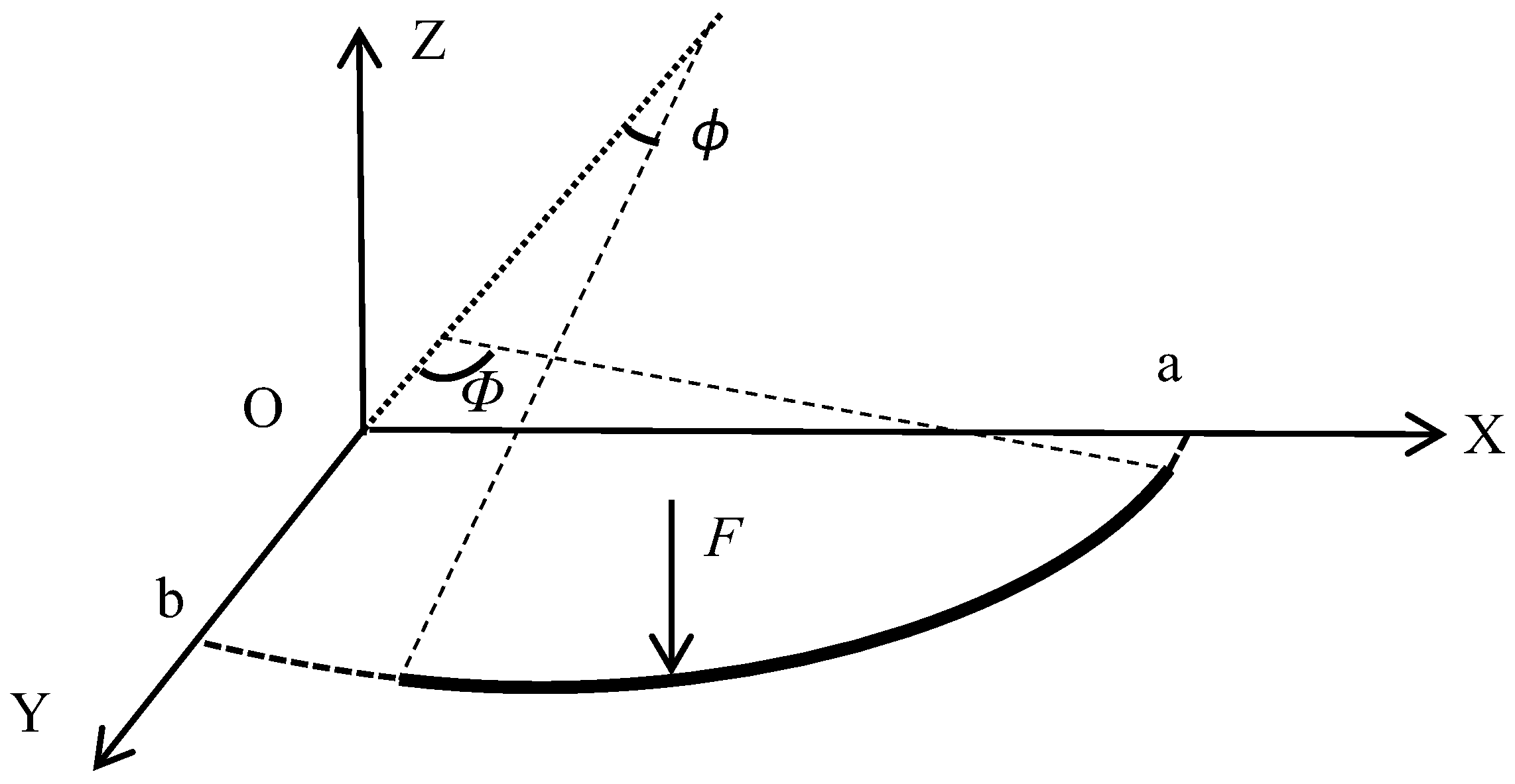
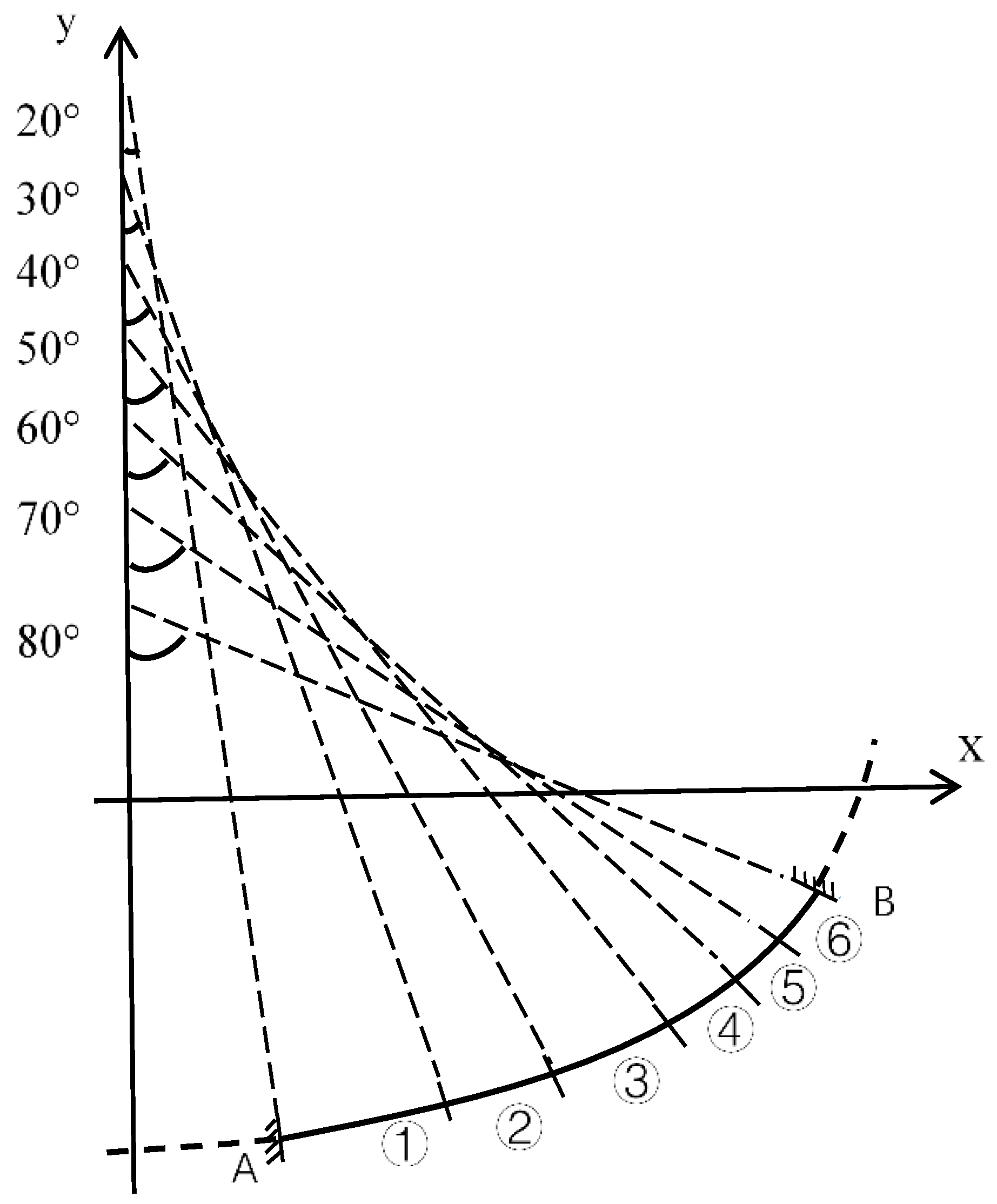
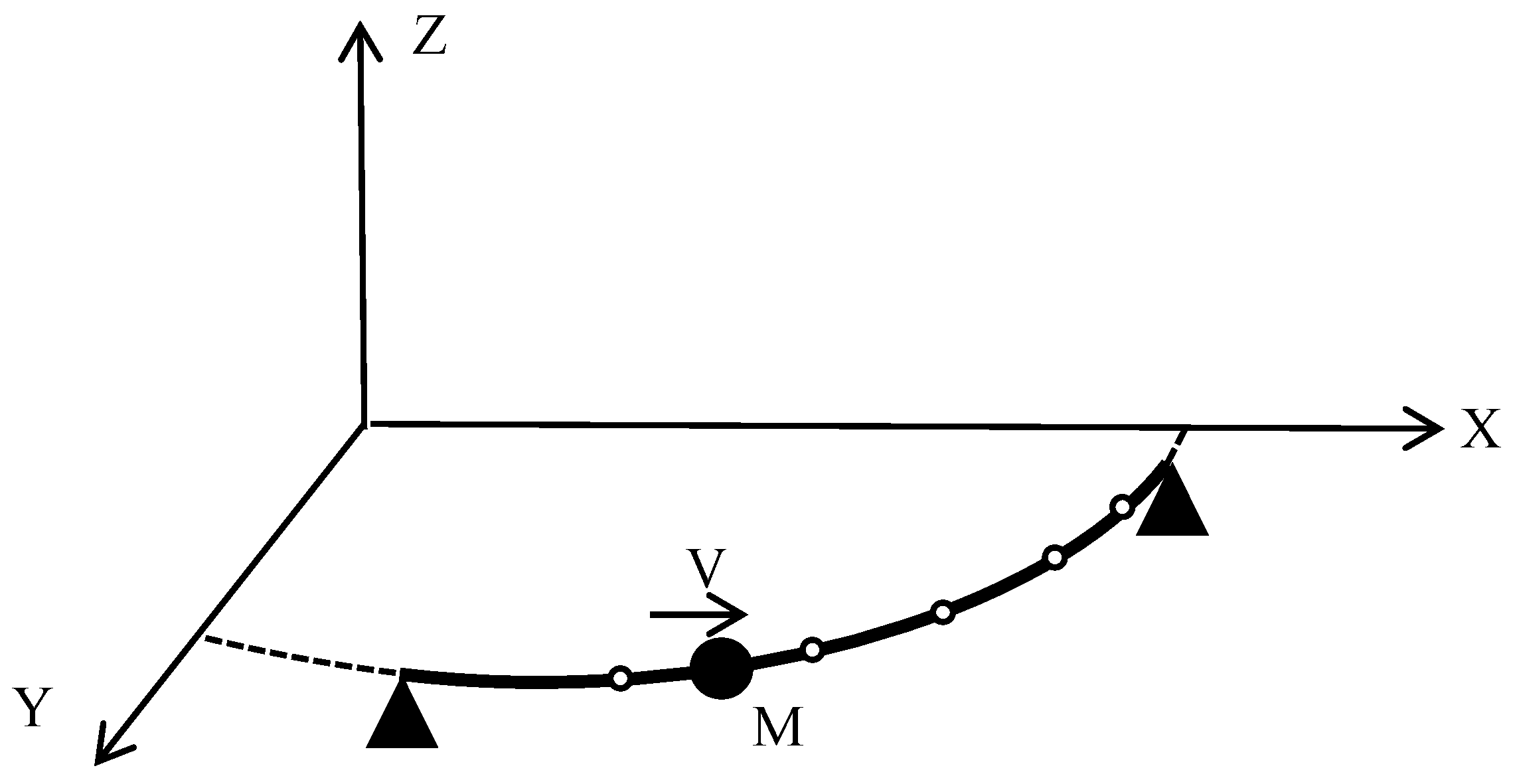
An elliptical curved girder bridge section conforming to the elliptical linear variable curvature was selected for study, and the elliptical curved girder model was simplified based on the assumption that the central axis of shear of a curved girder bridge coincides with the shaped centroid axis of the section. The simplified model was chosen in a right-angle coordinate system. An elliptical arc was taken from an ellipse with a semi-long axis length a and a semi-short axis length b. The ellipse is a symmetric figure, and in order to make the intercepted arc segment general, we chose one-fourth of the structure for the interception, as shown in
Figure 6, by selecting the part of the plane in any quadrant of the Cartesian coordinate system and choosing the points on the ellipse whose angles between the normal and negative directions of the
Y-axis are
φ and
Φ, respectively, as the endpoints of the intercepted arc segment.
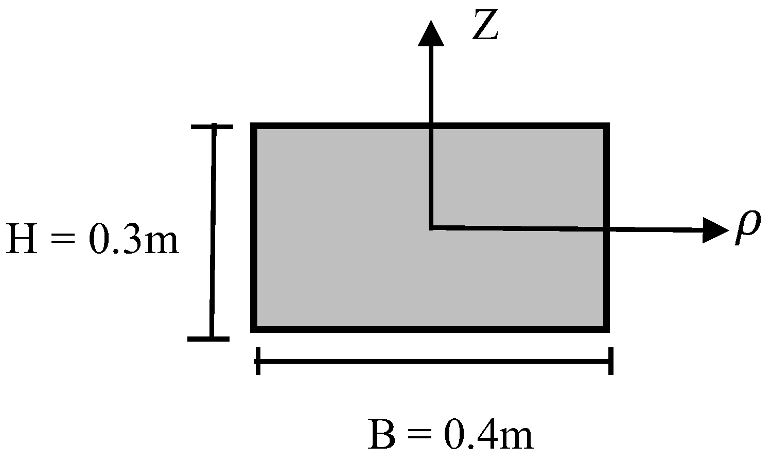
To facilitate the study of the overall dynamic response of the beam, a rectangular section was used in this study, while other sections could also be converted or equated to rectangular sections. The example used a rectangular section with a variable curvature steel beam, with section height H = 0.3 m, width B = 0.4 m, cross-sectional area A = 0.12 m
2, angle
φ of the left end with respect to the
Y-axis of 20°, angle
Φ of the right end with respect to the
Y-axis of 80°, long elliptical axis length a = 60 m, and short axis length b = 30 m. The rectangular cross-sectional dimensions are shown in
Figure 7.
The physical and geometric parameters of the bridge are shown in
Table 1.
The variable-curvature beam was divided into six elements, following the method of dividing one element for every 10° change of curvature on the beam. The division of the entire beam unit is shown in
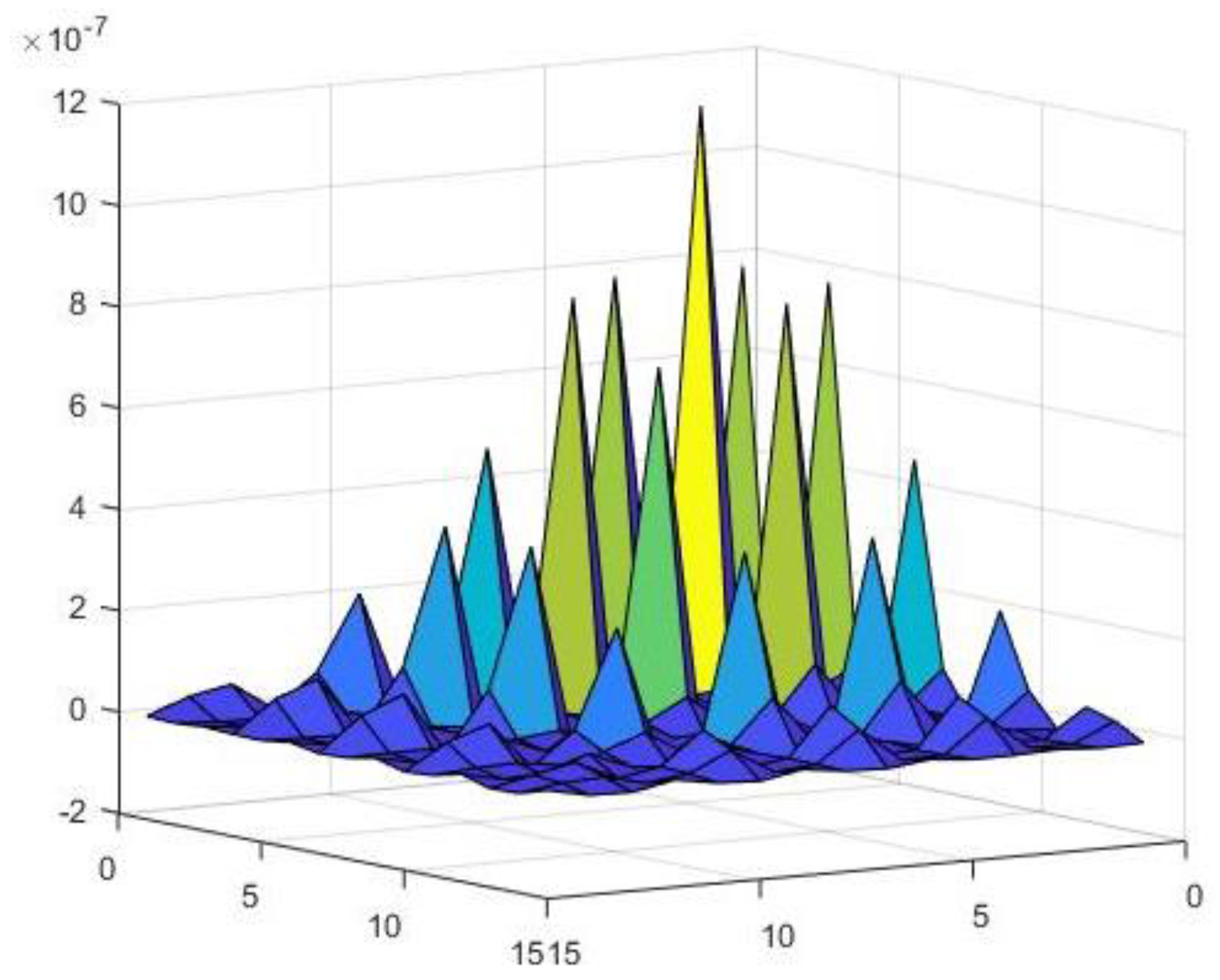
Figure 8, with element numbers ① to ⑥ from left to right. Therefore, the flexibility of the structure could be solved according to the structural mechanics force method and the principle of virtual work, and it could be integrated to obtain a flexibility matrix of dimensions 15
× 15.
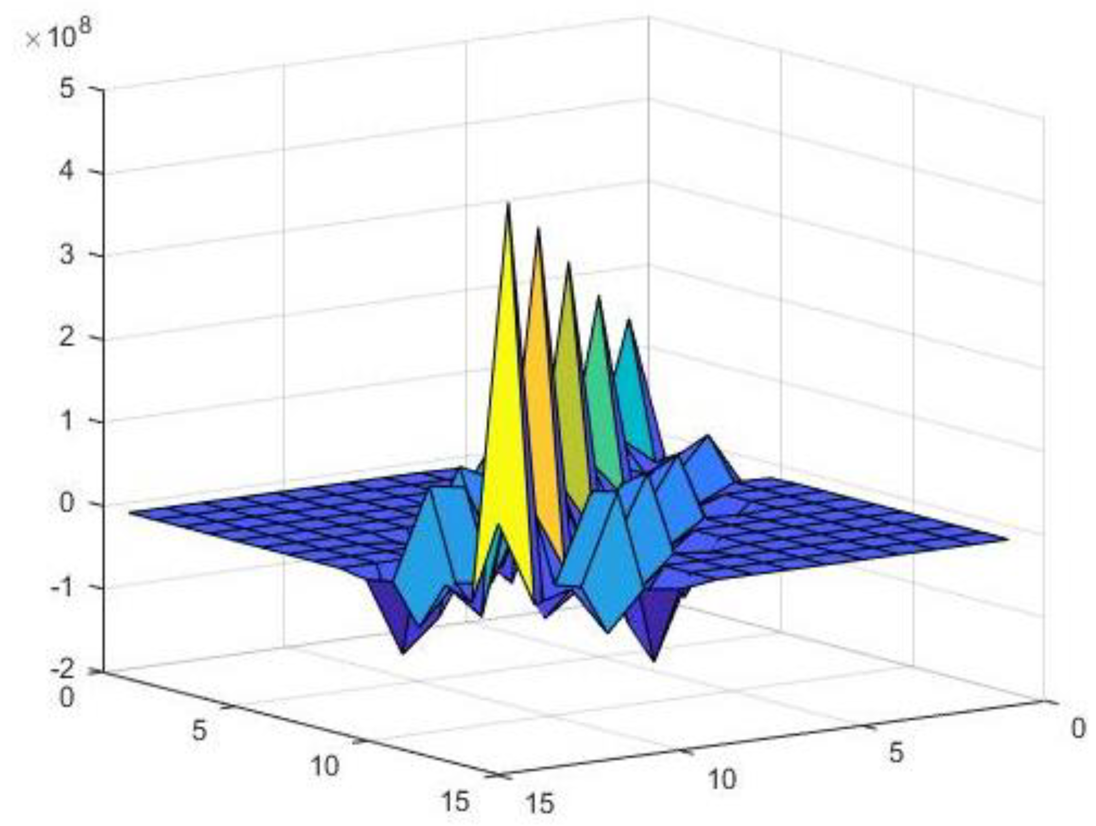
Figure 9 shows the flexibility matrix of the numerical model. From Equation (18), the inverse of the flexibility matrix yields a stiffness matrix
θ with a dimension of 15 × 15, as shown in
Figure 10.
The variable-curvature beam structure is divided into six segments, with knots as connection points. The mass of each arc segment can be assumed to be gathered into a point mass determined by statics at each of the junction points. The concentrated mass matrix is shown in
Figure 11.
4.1. Uniform Action of Moving Loads with Negligible Mass
The purpose of dynamic analysis of variable-curvature beam structures is to guide the design of curved bridges, where moving loads differ by many orders of magnitude compared with the self-weight of the curved beam, and the mass of the moving loads can be ignored and considered as concentrated forces. In addition to the self-weight load of the structure and the magnitude of the vehicle load, the effect of the moving speed on the dynamic response of a curved bridge is critical.
The response of an undamped variable-curvature beam with fixed restraint under a uniform-velocity moving load was calculated by moving a concentrated load of constant size from A to B. The beam cells were angularly varied equally by adjusting the time step so that the load moved exactly by one cell distance in each time step, as shown in
Figure 12.
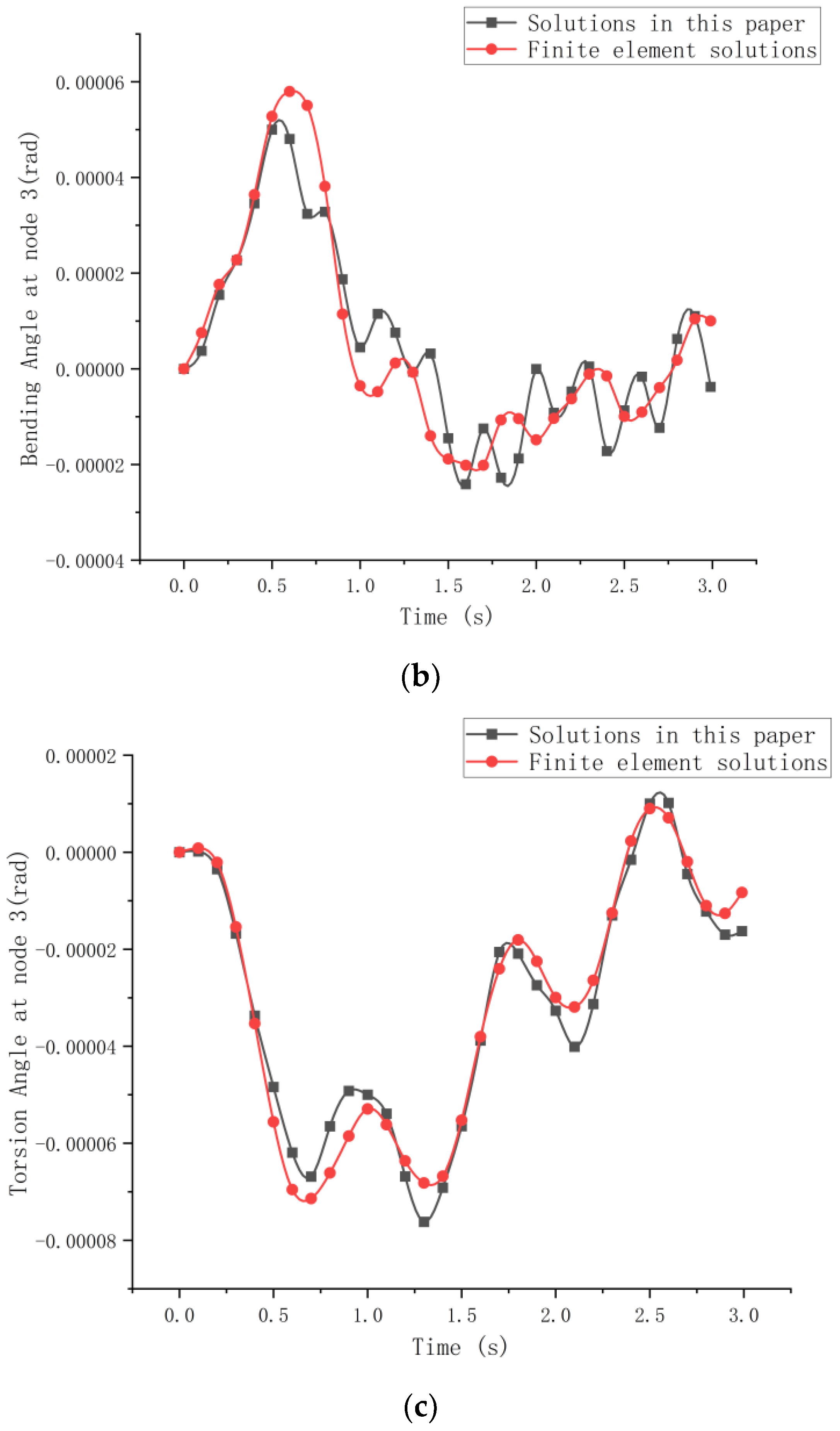
The black triangles in the figure represent the constraints at both ends of the curved beam, and the out-of-plane part is generally considered as a fixed constraint. The white dots indicate the nodes between the units after dividing the units on the beam. To verify the proposed method, finite element software was applied to simulate the moving load acting on the variable-curvature beam, and the derived dynamic response was compared to the precise integration method of this study. A finite element model with the same line type and the same properties was also created in Ansys and divided into six-cell structures. Using the precise integration method, the speed of the moving concentrated force was set to 11 m/s, and the magnitude of the force was set to 1000 N. Moving from left to right on the beam, taking node
as an example, the time course curve was studied, and the displacement response comparison in
Figure 13 was obtained.
The calculation steps and calculation times of the two methods are compared to obtain the data in
Table 2.
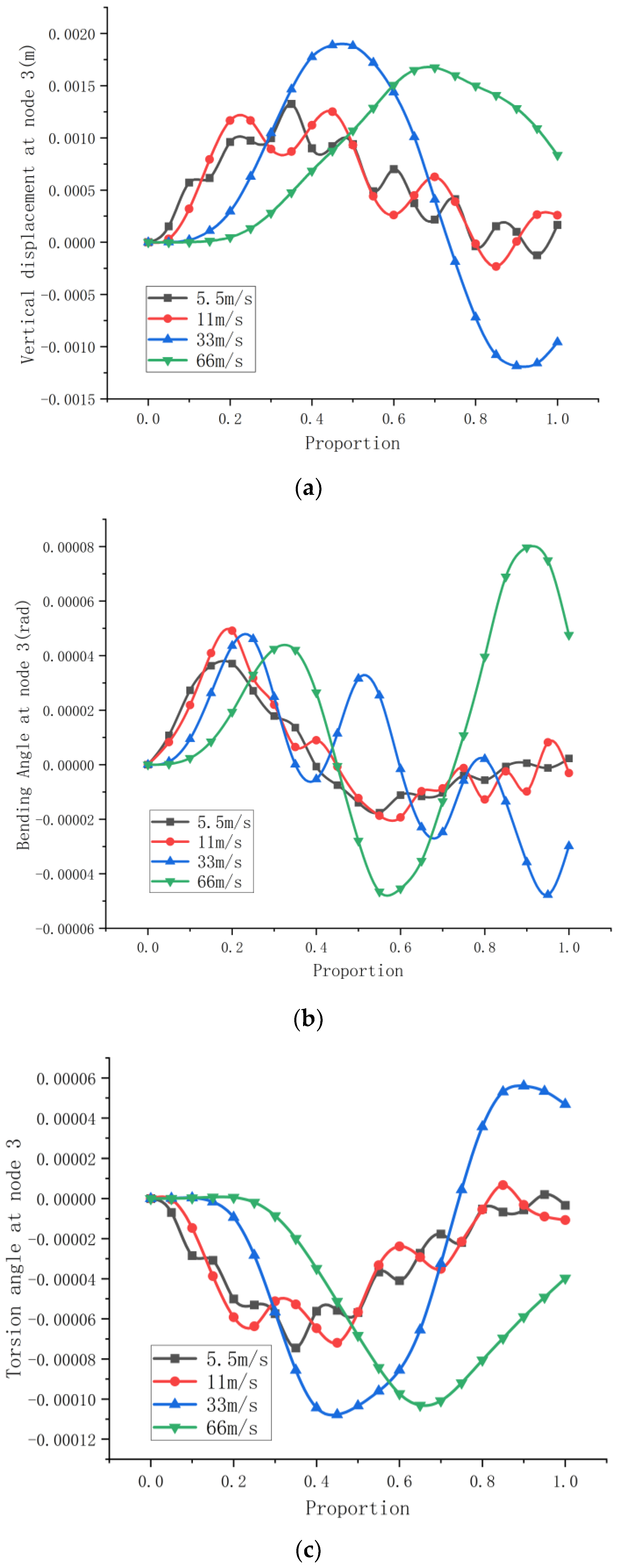
The dynamic response curves of beam node
with three degrees of freedom are shown in
Figure 14 for the cases when the external force
F of uniform velocity passes through the variable-curvature beam at 5.5 m/s, 11 m/s, 33 m/s, and 66 m/s. The x-coordinate in the figure is the ratio of the arc length moved by the dynamic load to the total length of the curved beam arc.
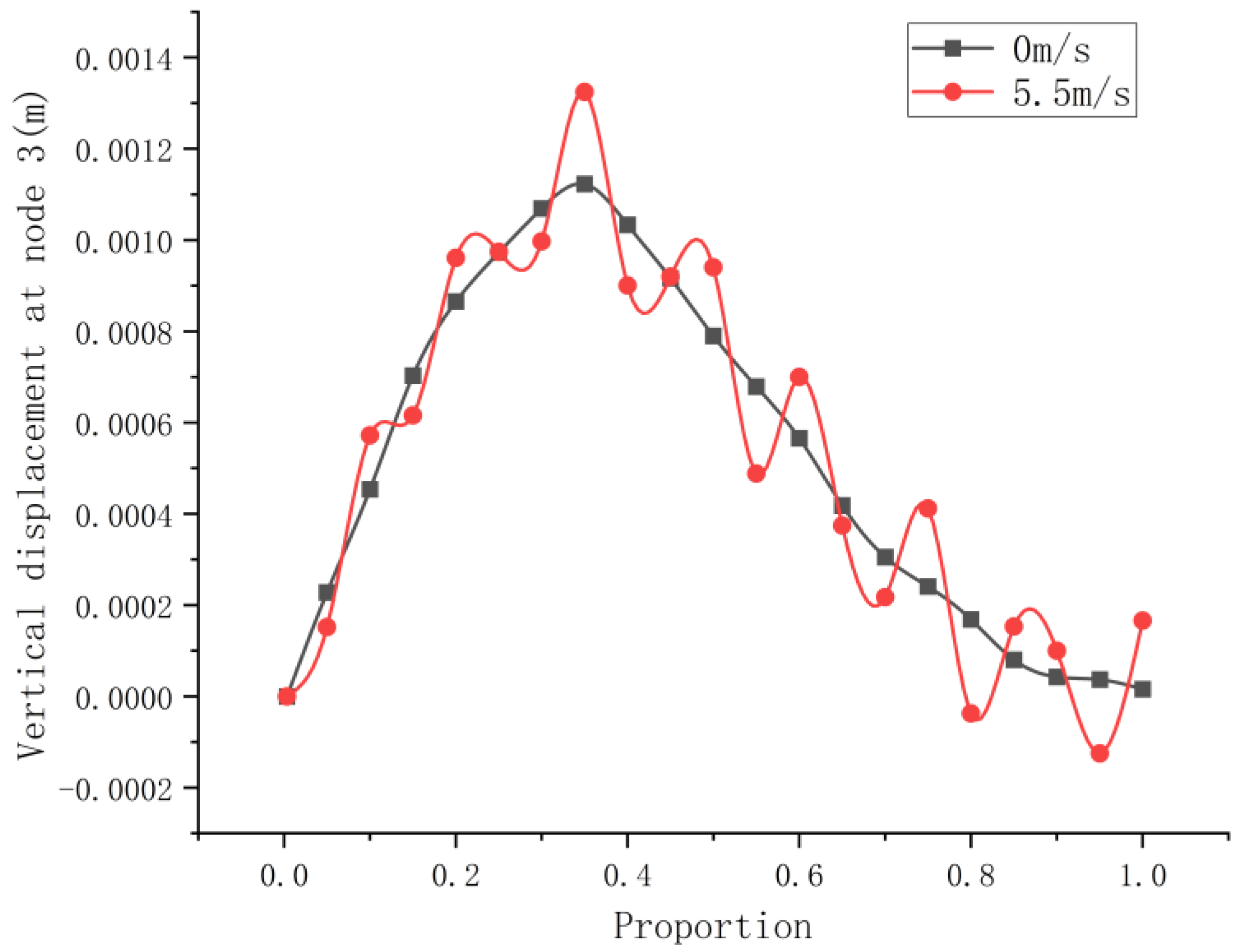
Figure 15 shows the vibration curves of the influence line in the static state and the vertical displacement of the beam in the small velocity case.
4.2. Dynamic Response under Moving Mass
The previous section provides a solution to the dynamic response under moving loads that neglects masses but affects the vertical displacement timescale of the curved beam when large-mass loads are applied to the beam. In practical engineering, moving objects coupling the mass of the moving load to the mass matrix of the bridge are more accurate in modeling the vibration response of a bridge under vehicle loads. Therefore, solving the dynamic time responses of the three directions of freedom of the curved beam under the action of a large-mass load is of great importance in analyzing the vibration response generated by a heavy vehicle passing along the curved beam. The structural analysis of a uniform mass m with different velocities of vertical forces acting on a variable-curvature beam is shown in
Figure 16.
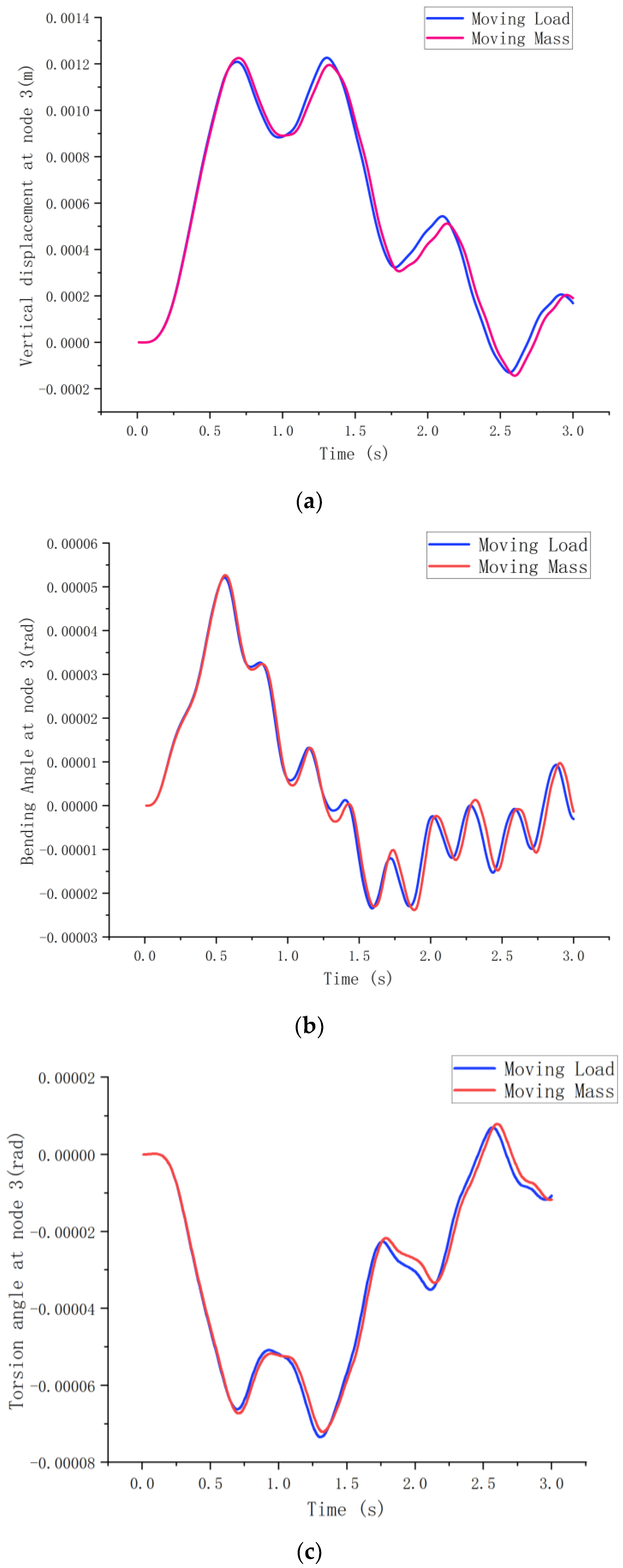
The mass matrix of the curved beam changed with time as the large-mass load moved across the beam. The speed of movement of the large mass was set to 11 m/s, and the movement was from left to right. Taking node 3,
, as an example, a time-course curve was determined, which provided a comparison of the displacement response of the moving load and the moving mass in
Figure 17.
As seen in
Figure 17, the displacement–time courses of forced vibrations of the variable-curvature beam with the time-dependent mass matrix taken into account were broadly consistent with the displacement vibration trends compared to the moving load alone. However, owing to the effect of the mass matrix, the vibration of the moving mass was relatively lagged, and the displacement amplitudes were small in all three directions of freedom.
5. Experimental Model
In addition to verification by the finite element method, the theoretical correctness of the study and the accuracy of its computational solutions could be verified through experimental data from an actual model built using a steel structure of variable curvature in the laboratory and subjecting the model to loading tests with moving loads.
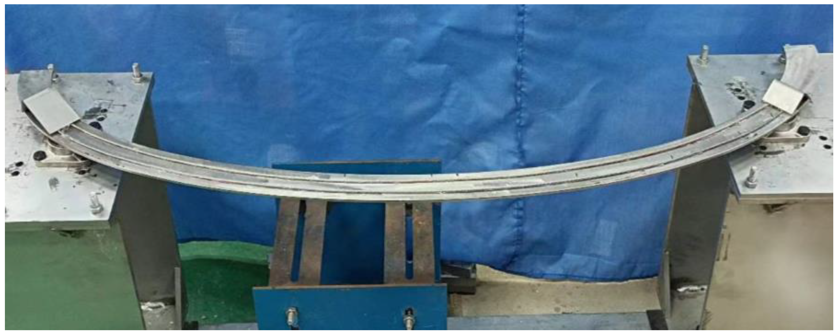
A curved steel beam of elliptical linear shape with a long half-axis of 60 cm and a short half-axis of 30 cm was designed under the conditions available in the laboratory. The beam had a constant rectangular cross-section with a width of 5 cm and thickness of 0.5 cm. Considering that the spatially curved beam would be subjected to vertical forces, moments around the radial direction, and torques around the tangential direction at each section, the spatially curved beam had to be a three-time super-stationary structure. One in-plane rotatable support was provided at the beam’s 40° and 140° positions. The arrangement of the laboratory curved-beam model is shown in
Figure 18.
The parameters of the bridge are shown in
Table 3.
As shown in
Figure 19 and
Figure 20, a sliding ramp was placed at the left end of the beam, and two lubricated wire ropes were fixed at the same spacing on the upper surface of the beam as a track for the sphere to slide. Next, 0.75 kg balls were released at the left end at different speeds. Lubricant was applied to the balls and track to minimize the effect of friction on the sliding track. Vertical displacement sensors were placed at the span and 80° positions of the curved beam, and the length of time the ball traveled the full length of the curved beam and the change in vertical displacement at the sensor placement were recorded. The velocity of the ball was changed, and the vertical displacement data were then measured again.
Theoretical calculation results according to the theory in this study were based on the model dimensions, weight of the ball, and length of movement. The experimental data were compared to the theory, as shown in
Figure 21. From the comparison, as the speed of the moving ball increased, the vertical displacement–time curve showed small oscillations, which was consistent with the theoretical results in the previous study.


