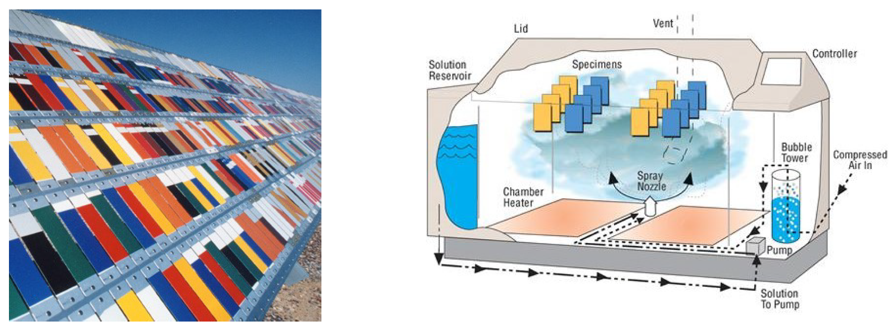
Figure 1.
Outdoor weathering rack (
left) and a salt-spray tester (
right) [
17,
18].
Figure 1.
Outdoor weathering rack (
left) and a salt-spray tester (
right) [
17,
18].
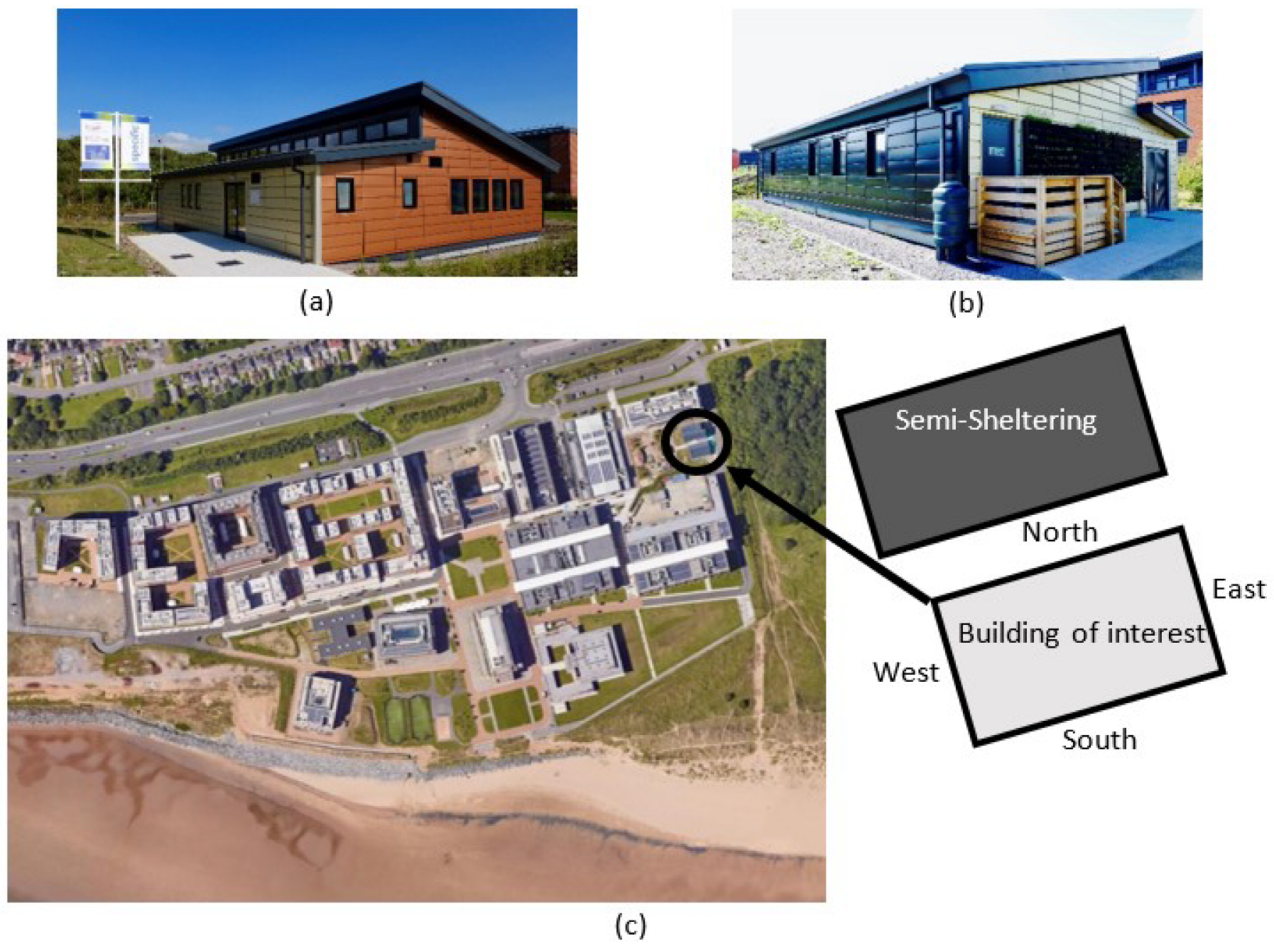
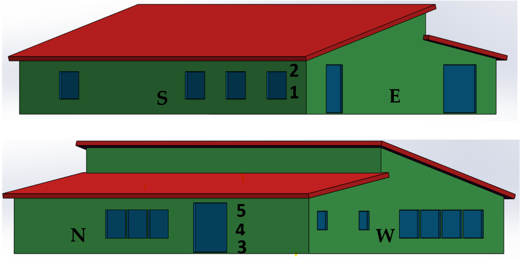
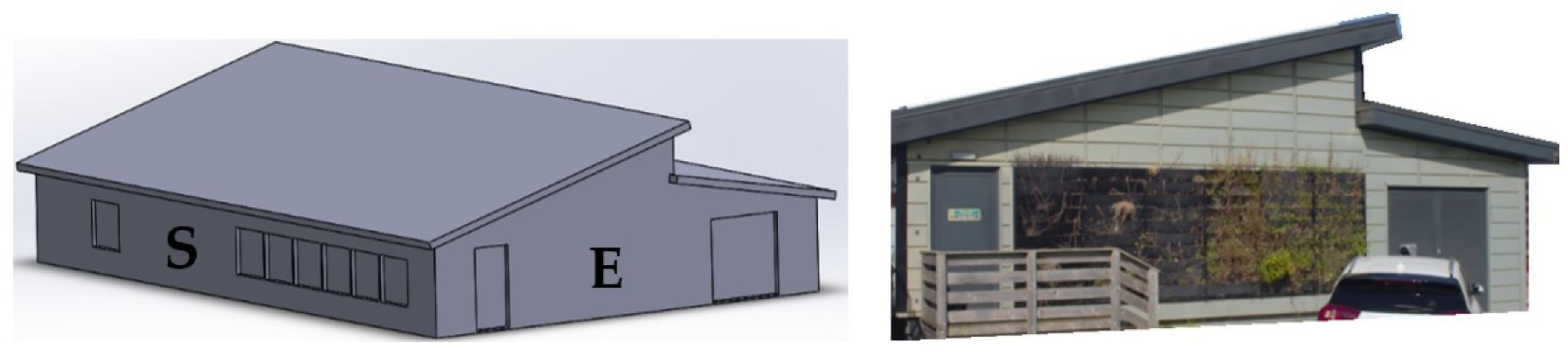
Figure 2.
Building viewed from the (a) northwest, (b) southeast, and (c) location of the building and the façade names used for reference.
Figure 2.
Building viewed from the (a) northwest, (b) southeast, and (c) location of the building and the façade names used for reference.
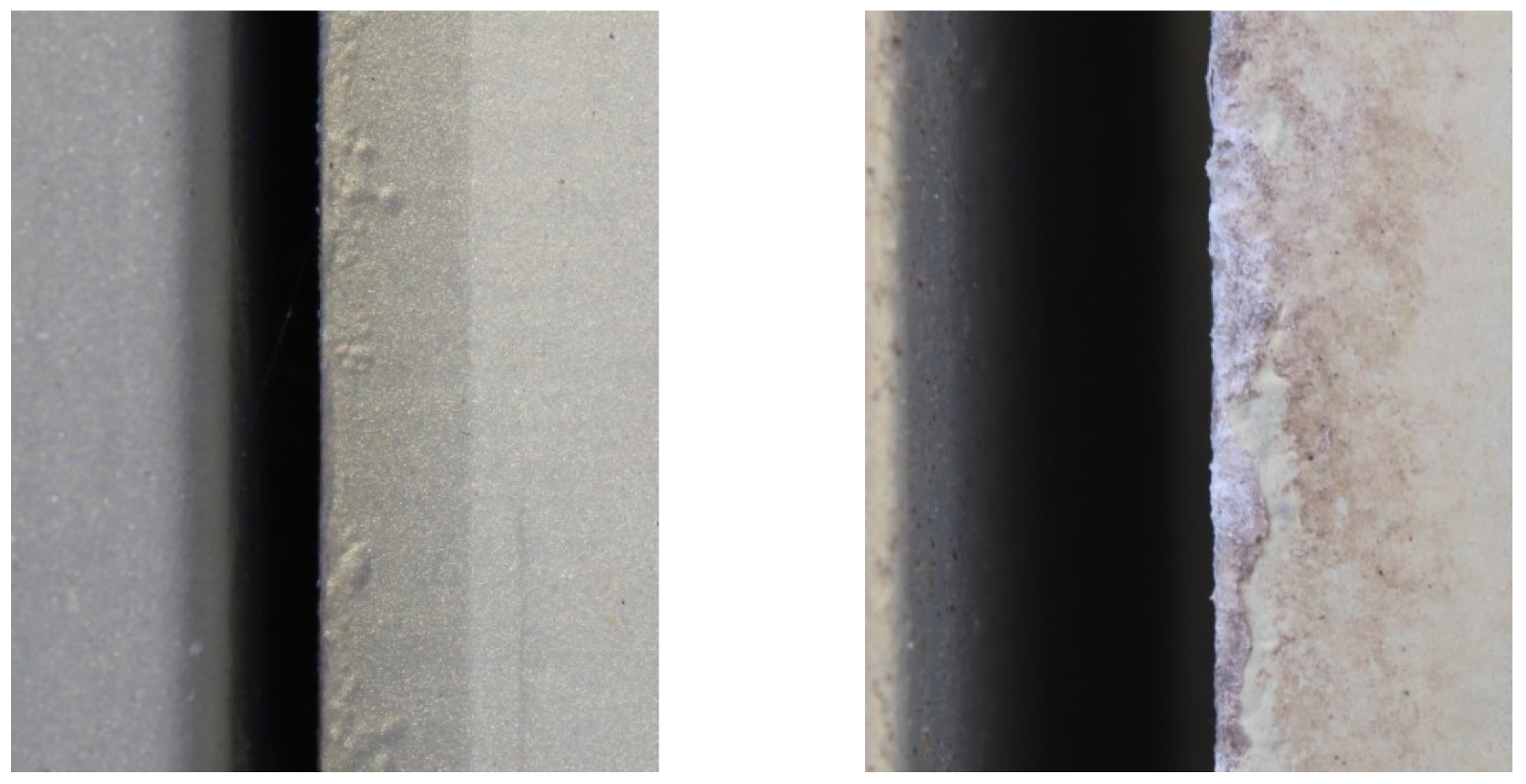
Figure 3.
Examples of the two main types of cut edge degradation observed: blistering (left) and white rust (right).
Figure 3.
Examples of the two main types of cut edge degradation observed: blistering (left) and white rust (right).
Figure 4.
Location of the five sensing boxes on the building. The building is coloured according to materials with green indicating PVDF cladding, red indicating integrated PV roofing, blue indicating windows and doors, and dark purple indicating the soffit region composed of PVC cladding material.
Figure 4.
Location of the five sensing boxes on the building. The building is coloured according to materials with green indicating PVDF cladding, red indicating integrated PV roofing, blue indicating windows and doors, and dark purple indicating the soffit region composed of PVC cladding material.
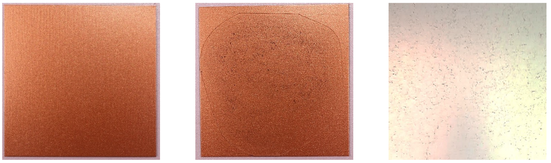
Figure 5.
Initially clean PVDF sample (left), PVDF sample with wet-applied 4000 mgm−2 of deposit (middle), and observed natural deposit on the building (right).
Figure 5.
Initially clean PVDF sample (left), PVDF sample with wet-applied 4000 mgm−2 of deposit (middle), and observed natural deposit on the building (right).
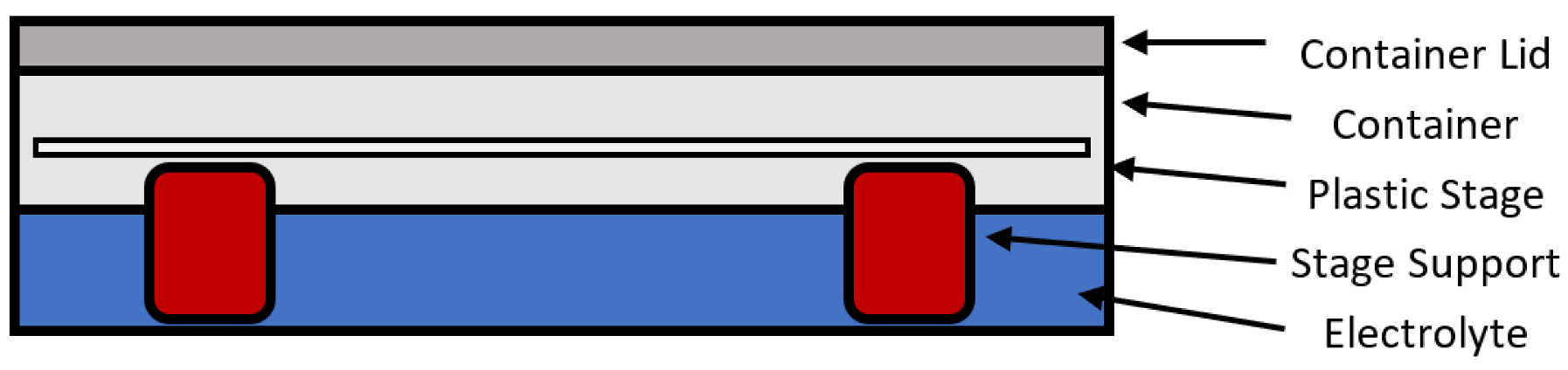
Figure 6.
Experimental setup of the humidity testing chamber.
Figure 6.
Experimental setup of the humidity testing chamber.
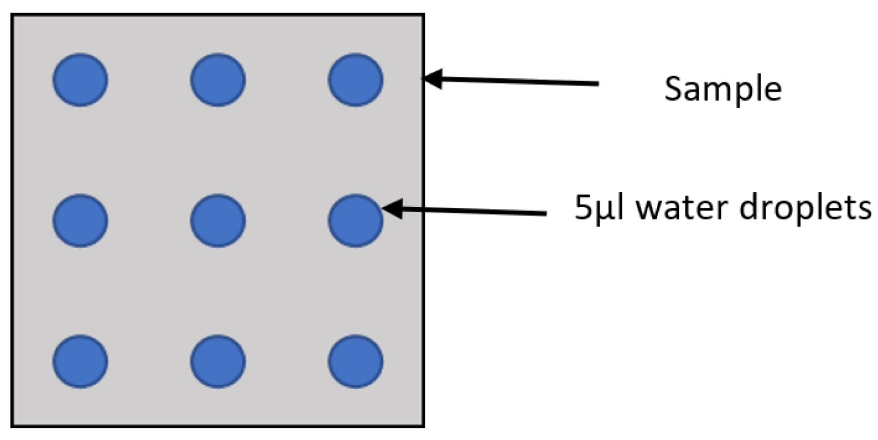
Figure 7.
Droplet test used to measure drying/water retention.
Figure 7.
Droplet test used to measure drying/water retention.
Figure 8.
Building model (left) and actual building (right).
Figure 8.
Building model (left) and actual building (right).
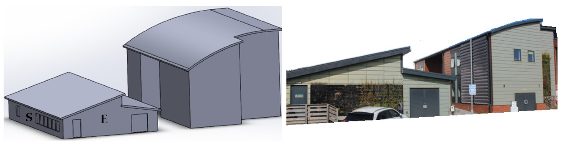
Figure 9.
Dual building model (left) and actual buildings (right).
Figure 9.
Dual building model (left) and actual buildings (right).
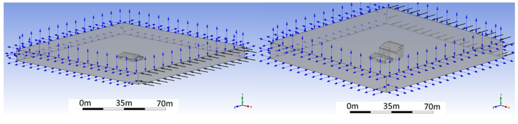
Figure 10.
The computation domain for the single (left) and dual building (right) models. The black arrows signify an inlet boundary condition whereas the blue arrows show an open boundary condition.
Figure 10.
The computation domain for the single (left) and dual building (right) models. The black arrows signify an inlet boundary condition whereas the blue arrows show an open boundary condition.
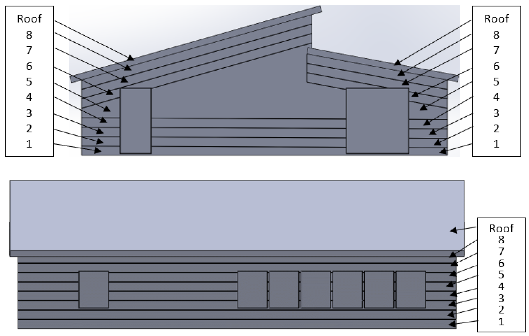
Figure 11.
Example of façade sectioning for the east (top) and south (bottom) façades.
Figure 11.
Example of façade sectioning for the east (top) and south (bottom) façades.
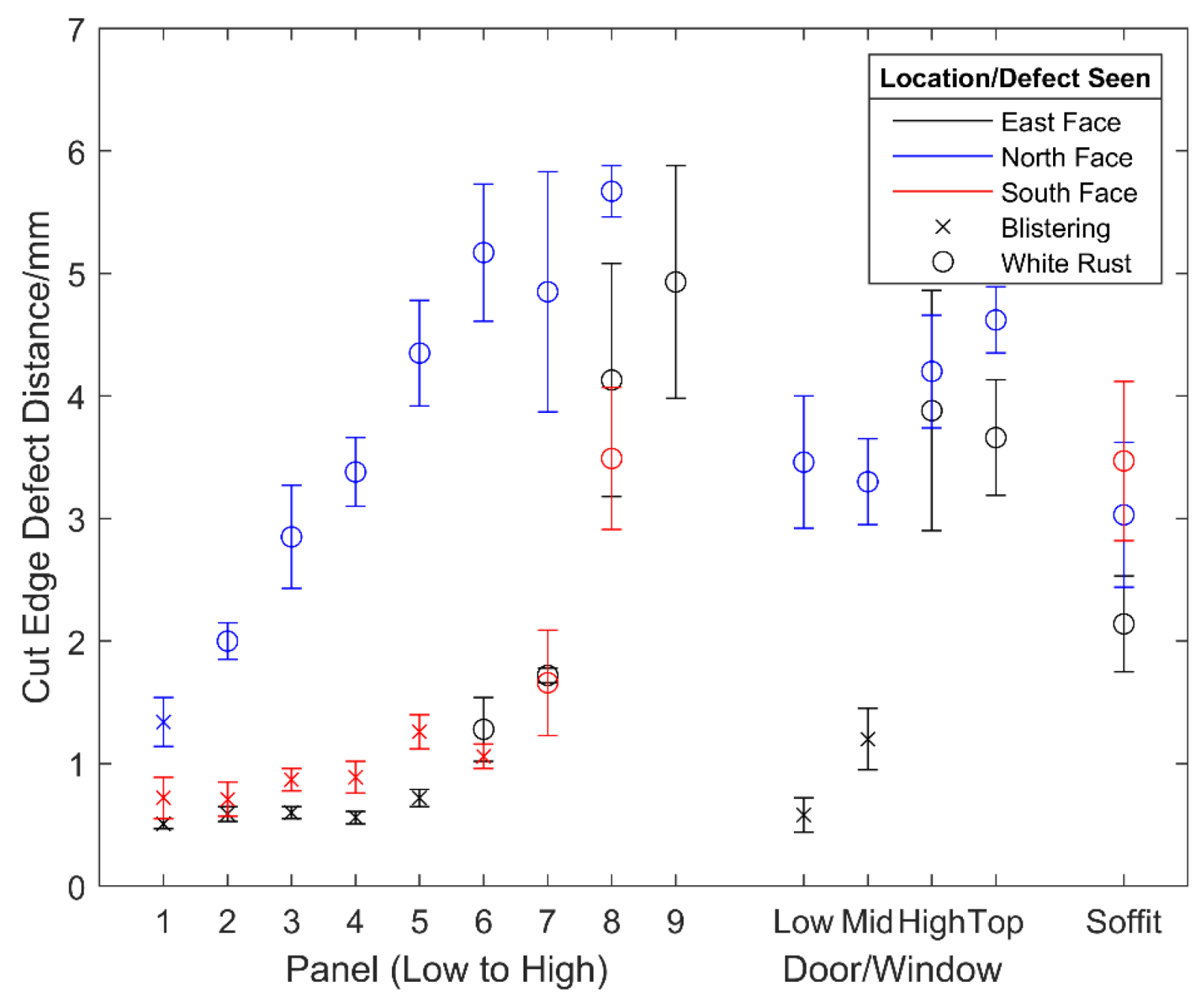
Figure 12.
Variation in cut edge defect size and type across the building.
Figure 12.
Variation in cut edge defect size and type across the building.
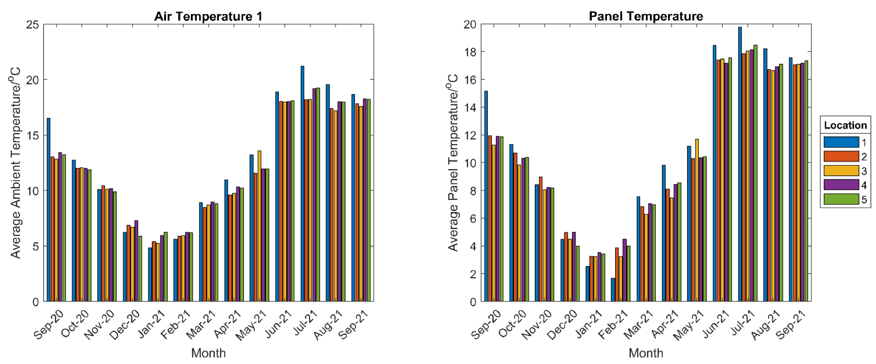
Figure 13.
Comparison of air (left) and panel (right) temperatures recorded at each location.
Figure 13.
Comparison of air (left) and panel (right) temperatures recorded at each location.
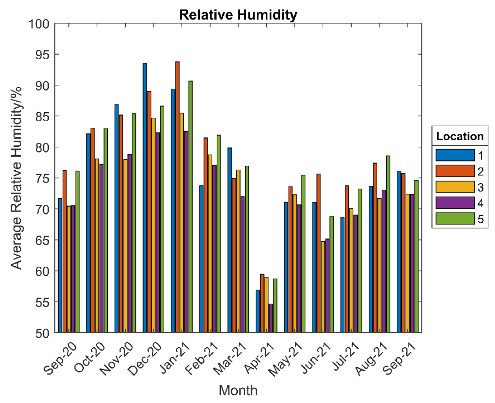
Figure 14.
Comparison of the relative humidity recorded at each location.
Figure 14.
Comparison of the relative humidity recorded at each location.
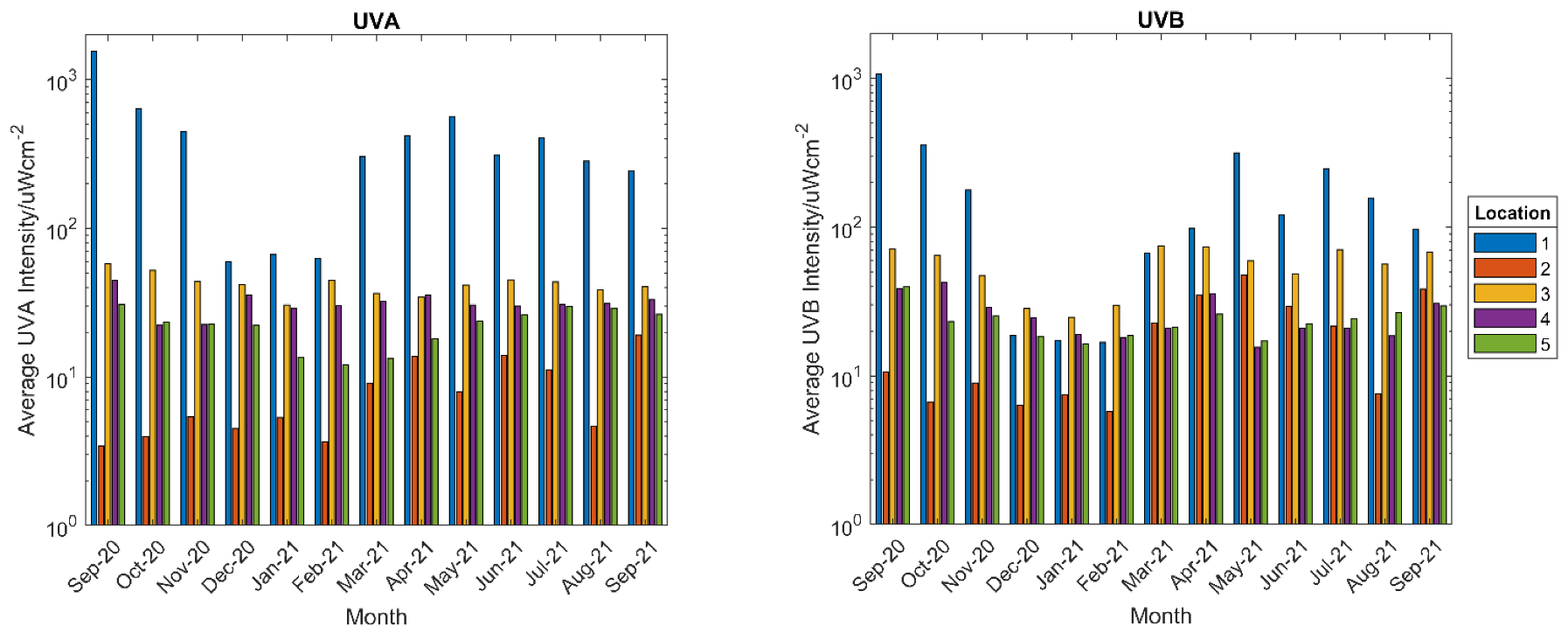
Figure 15.
Comparison of UVA (left) and UVB (right) intensity recorded at each location.
Figure 15.
Comparison of UVA (left) and UVB (right) intensity recorded at each location.
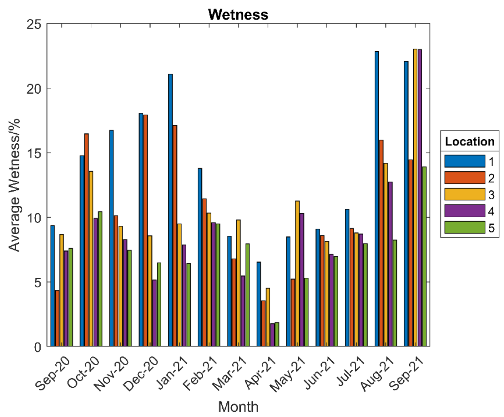
Figure 16.
Comparison of % wetness recorded at each location.
Figure 16.
Comparison of % wetness recorded at each location.
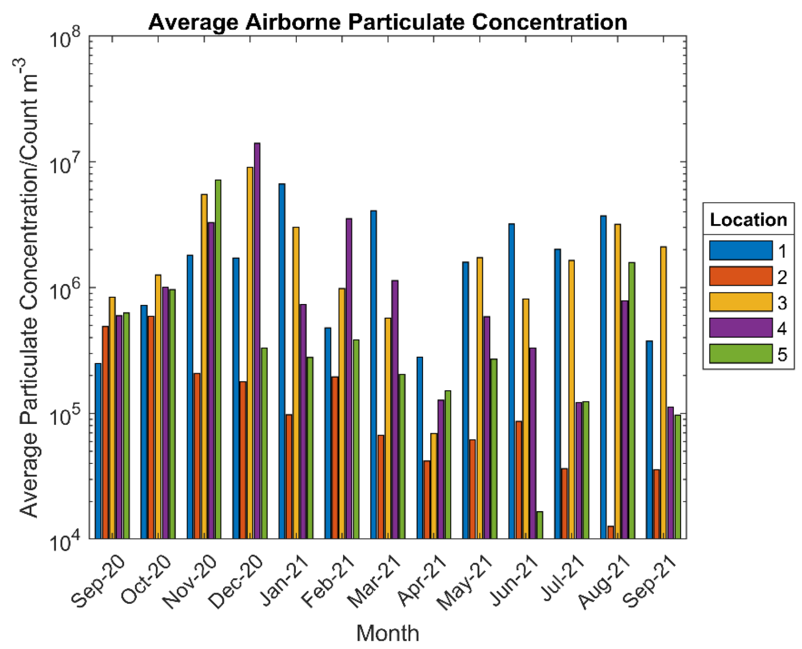
Figure 17.
Comparison of particulate concentration recorded at each location.
Figure 17.
Comparison of particulate concentration recorded at each location.
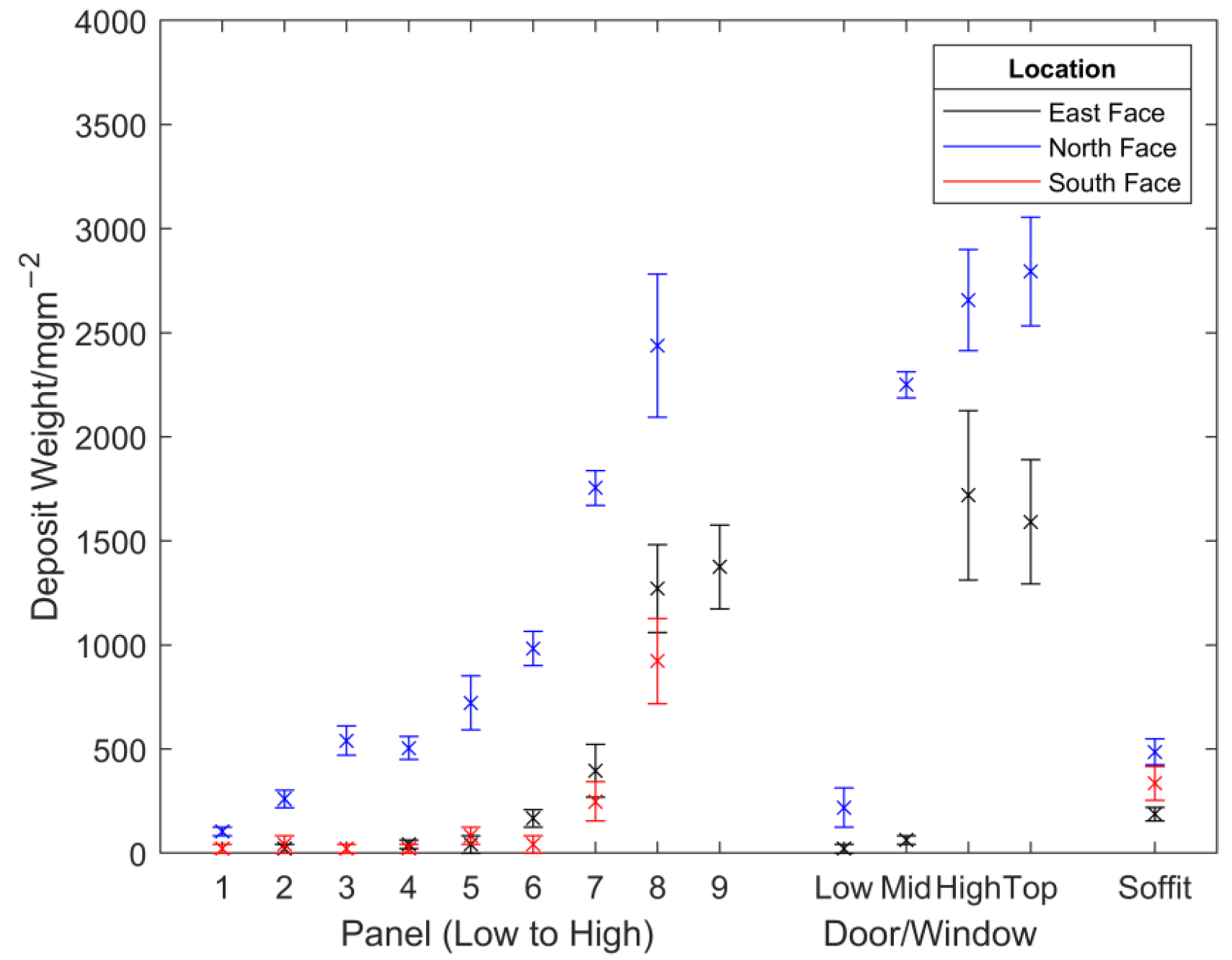
Figure 18.
Variation in the amount of deposit present across the building.
Figure 18.
Variation in the amount of deposit present across the building.
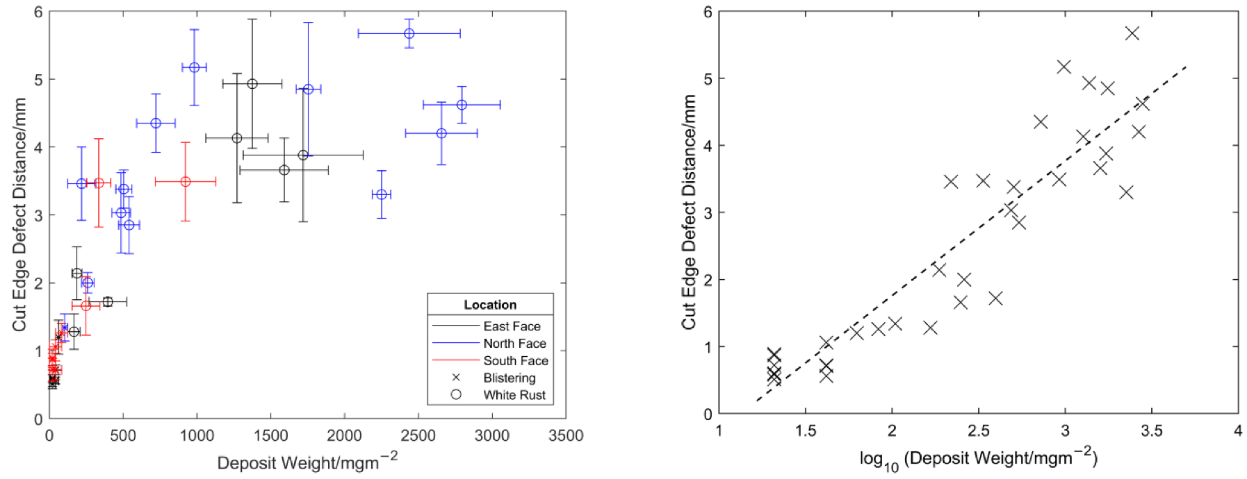
Figure 19.
Comparison of the cut edge defect distance to the measured deposit weight in each location (left) and a demonstration of the logarithmic trend between the two factors (right).
Figure 19.
Comparison of the cut edge defect distance to the measured deposit weight in each location (left) and a demonstration of the logarithmic trend between the two factors (right).
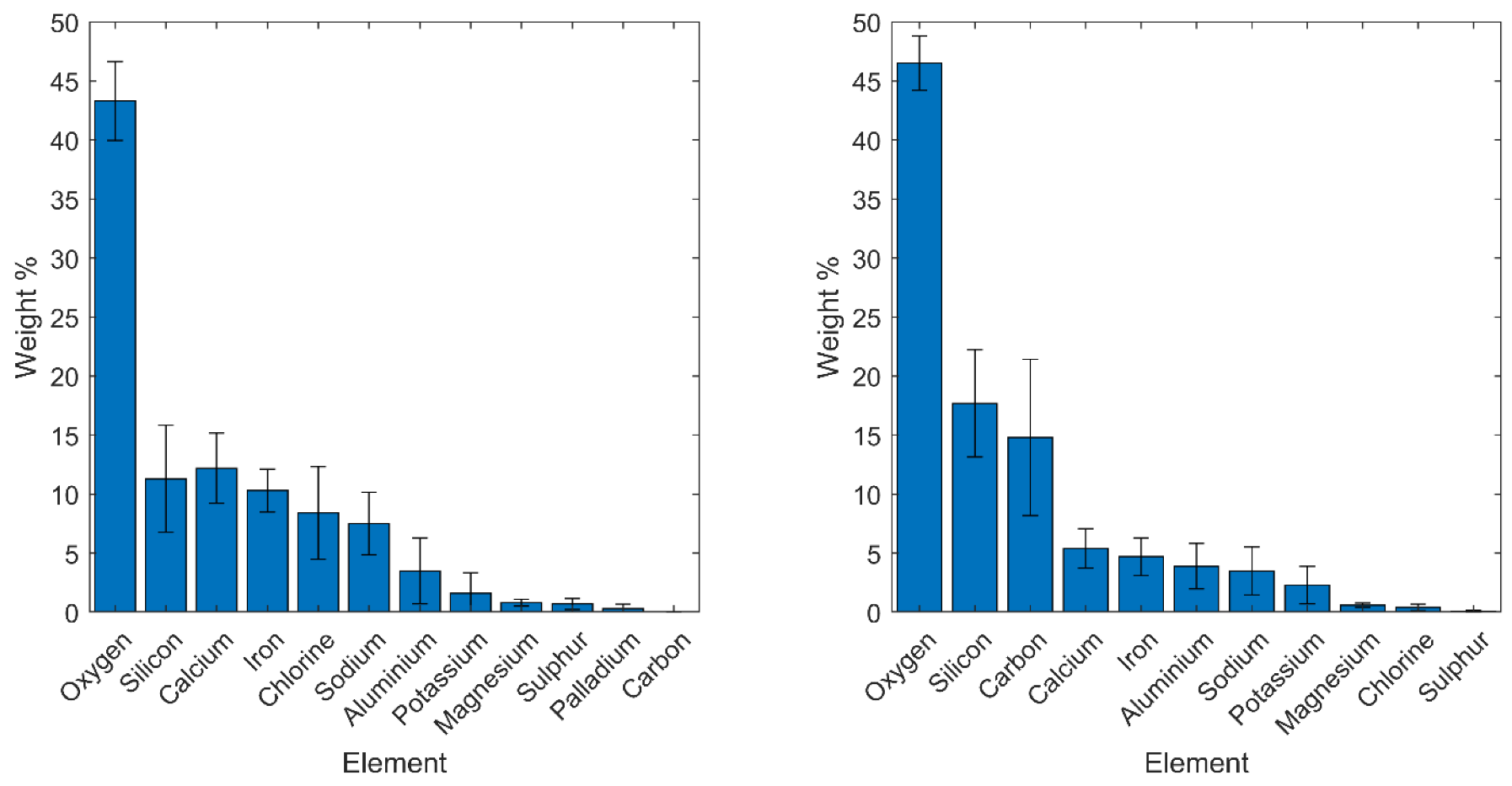
Figure 20.
EDS analysis of the SP sample (left) and the P sample (right).
Figure 20.
EDS analysis of the SP sample (left) and the P sample (right).
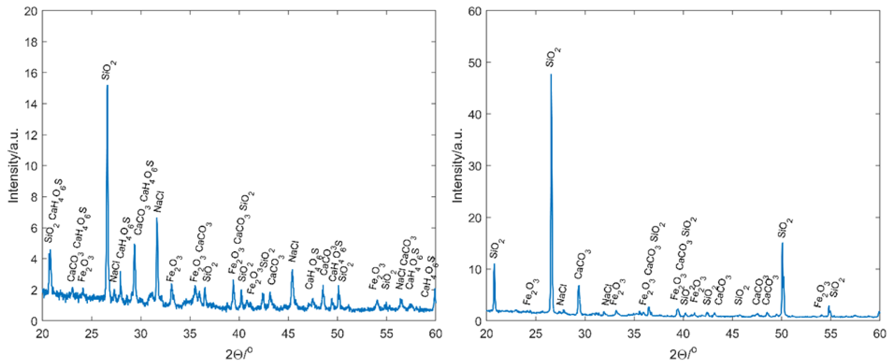
Figure 21.
XRD analysis of the SP sample (left) and the P sample (right).
Figure 21.
XRD analysis of the SP sample (left) and the P sample (right).
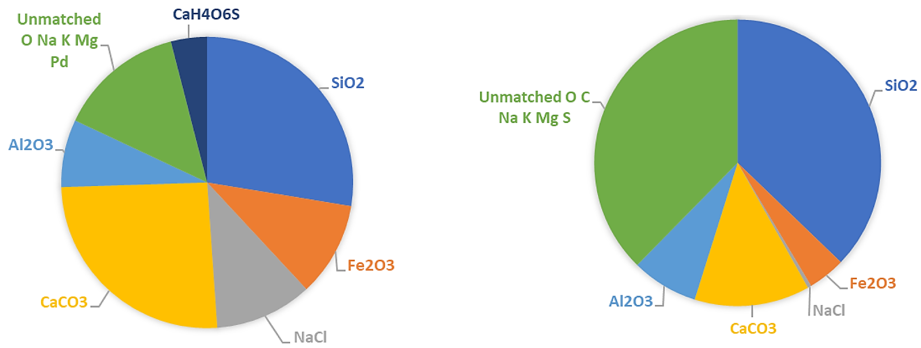
Figure 22.
Likely constituents of the analysis of the SP sample (left) and the P sample (right).
Figure 22.
Likely constituents of the analysis of the SP sample (left) and the P sample (right).
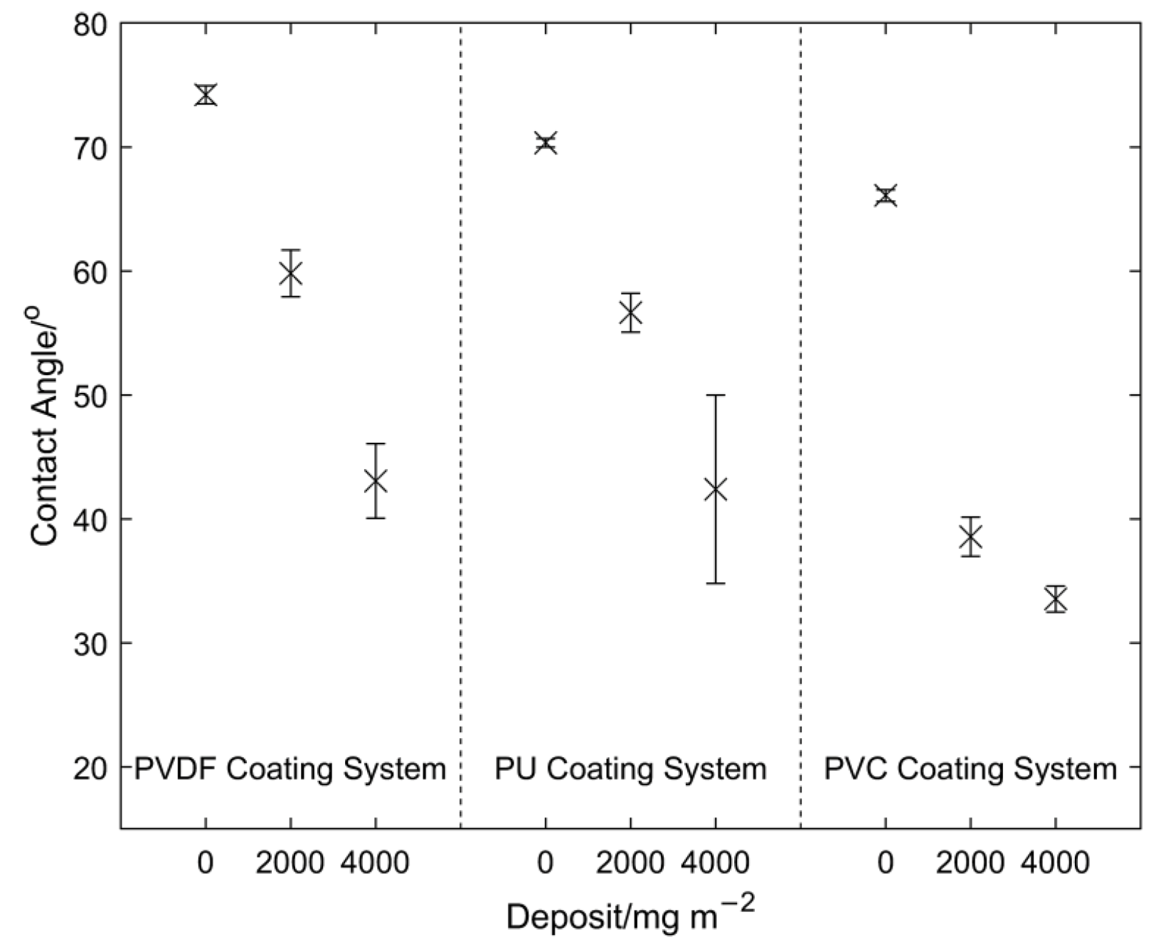
Figure 23.
The effect of increased deposit build-up on the wetting angle measurements for the three different coating systems.
Figure 23.
The effect of increased deposit build-up on the wetting angle measurements for the three different coating systems.
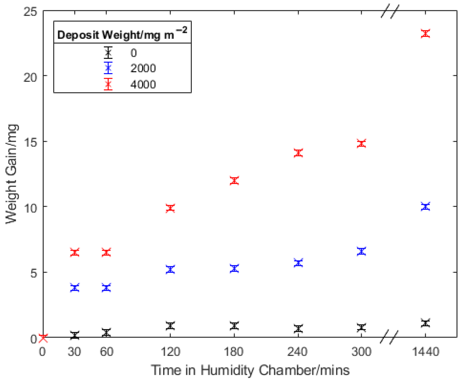
Figure 24.
Water adsorption as a result of deposit weight and time in a humidity chamber for the PVDF-coated samples.
Figure 24.
Water adsorption as a result of deposit weight and time in a humidity chamber for the PVDF-coated samples.
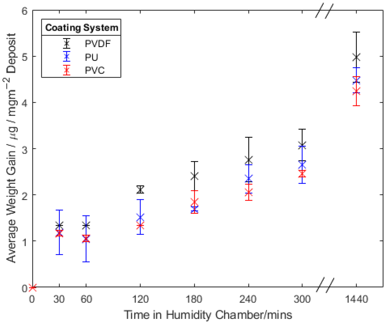
Figure 25.
Water adsorption per mgm−2 of deposit weight as a result of time in the humidity chamber for each coating system.
Figure 25.
Water adsorption per mgm−2 of deposit weight as a result of time in the humidity chamber for each coating system.
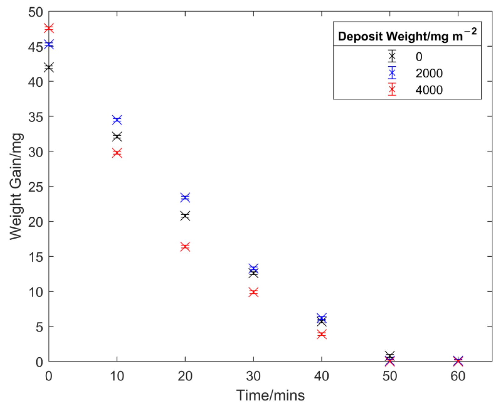
Figure 26.
Effect of deposit weight on the drying of applied water droplets for the PVDF-coated samples.
Figure 26.
Effect of deposit weight on the drying of applied water droplets for the PVDF-coated samples.
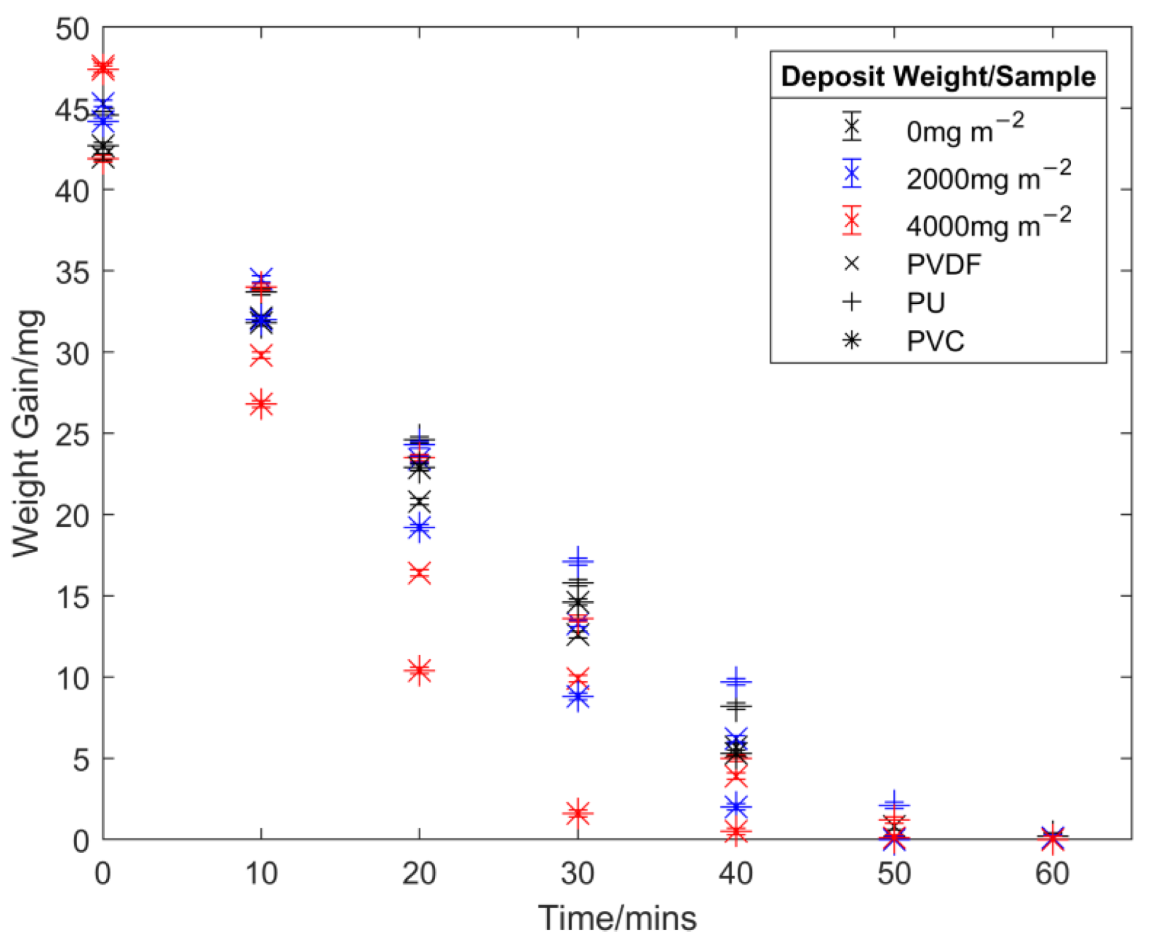
Figure 27.
Effect of deposit weight on the drying of applied water droplets for all coating systems.
Figure 27.
Effect of deposit weight on the drying of applied water droplets for all coating systems.
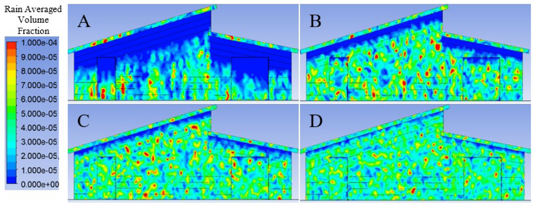
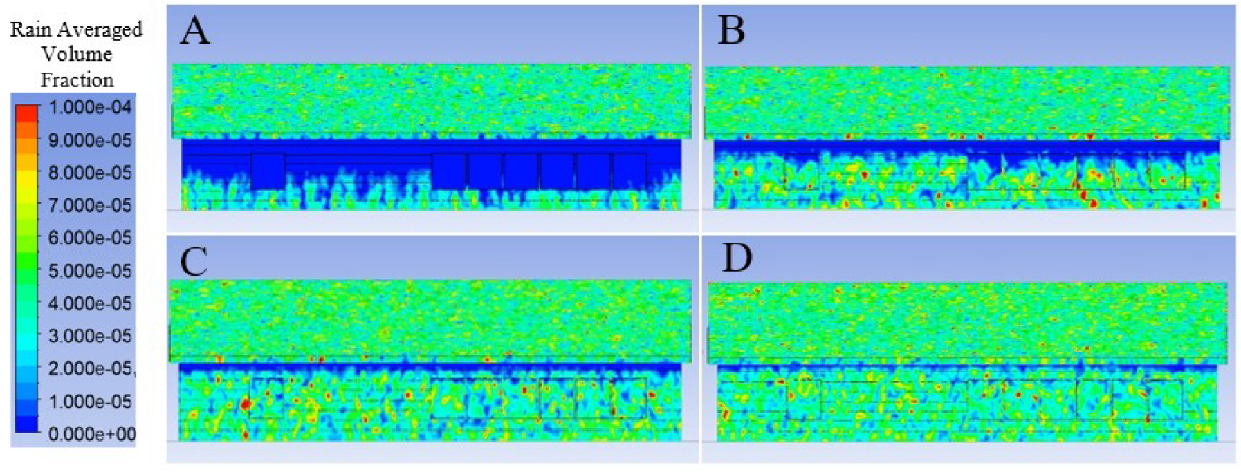
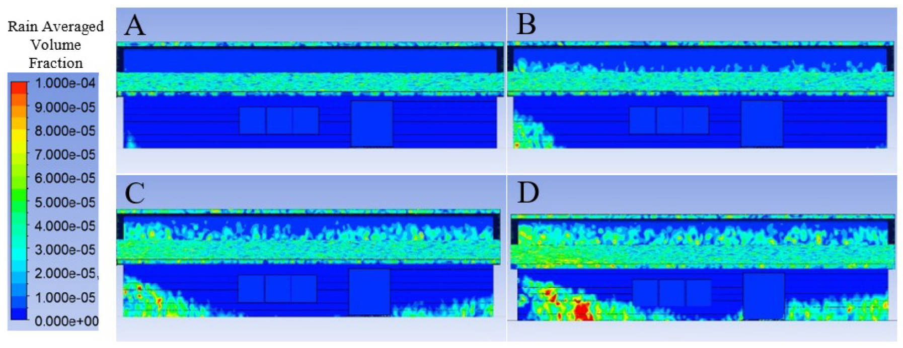
Figure 28.
Predicted rain impact density for the east elevation under 2 (A), 4 (B), 6 (C), and 8 (D) ms−1 wind speed applied normal to the east elevation.
Figure 28.
Predicted rain impact density for the east elevation under 2 (A), 4 (B), 6 (C), and 8 (D) ms−1 wind speed applied normal to the east elevation.
Figure 29.
Predicted rain impact density for the south elevation under 2 (A), 4 (B), 6 (C), and 8 (D) ms−1 wind speed applied normal to the south elevation.
Figure 29.
Predicted rain impact density for the south elevation under 2 (A), 4 (B), 6 (C), and 8 (D) ms−1 wind speed applied normal to the south elevation.
Figure 30.
Predicted rain impact density for the north elevation under 2 (A), 4 (B), 6 (C), and 8 (D) ms−1 wind speed applied normal to the north elevation.
Figure 30.
Predicted rain impact density for the north elevation under 2 (A), 4 (B), 6 (C), and 8 (D) ms−1 wind speed applied normal to the north elevation.
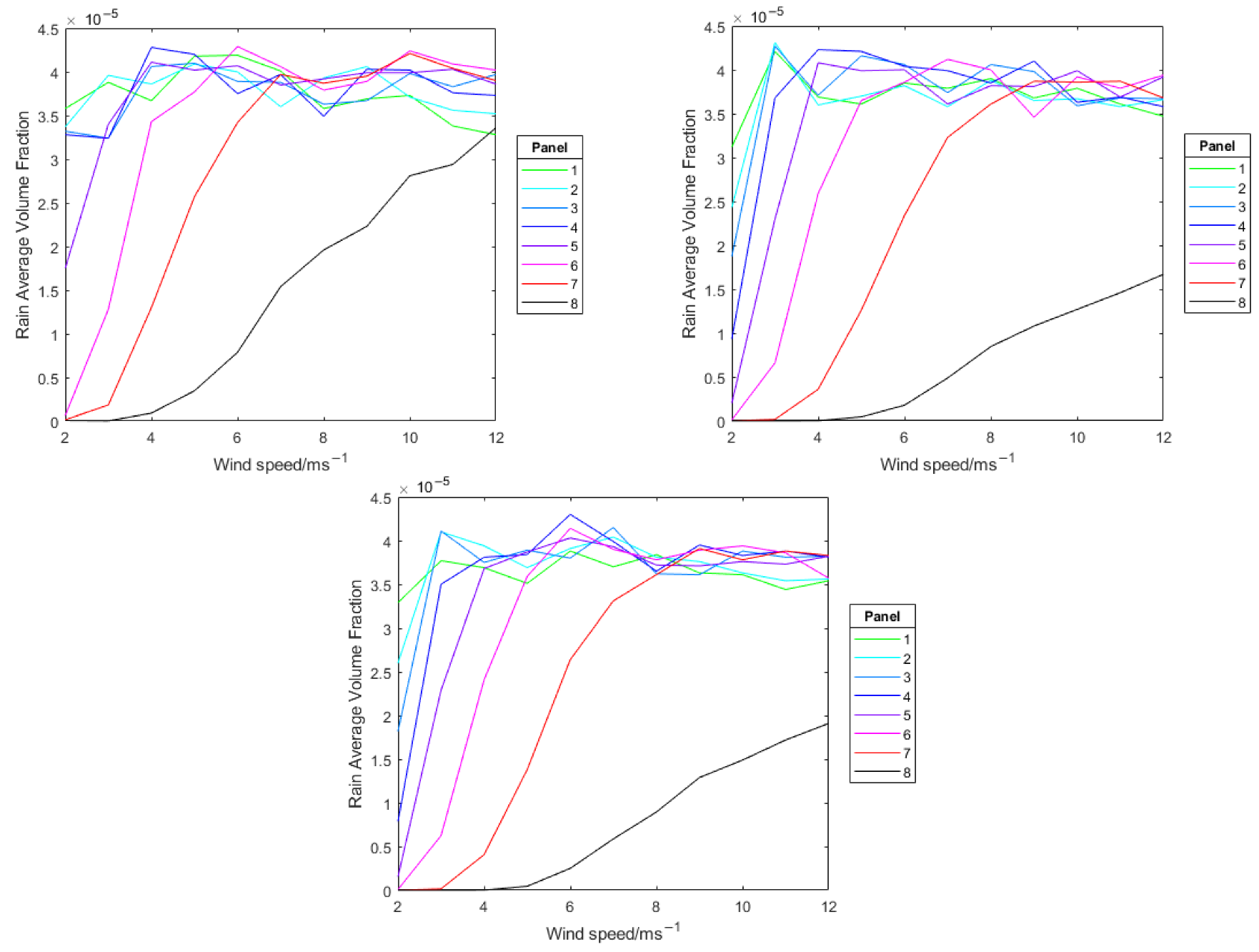
Figure 31.
Measured average rain volume fraction at each location for the east (top left), south (top right), and north (bottom) façade.
Figure 31.
Measured average rain volume fraction at each location for the east (top left), south (top right), and north (bottom) façade.
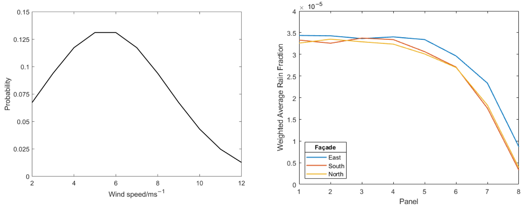
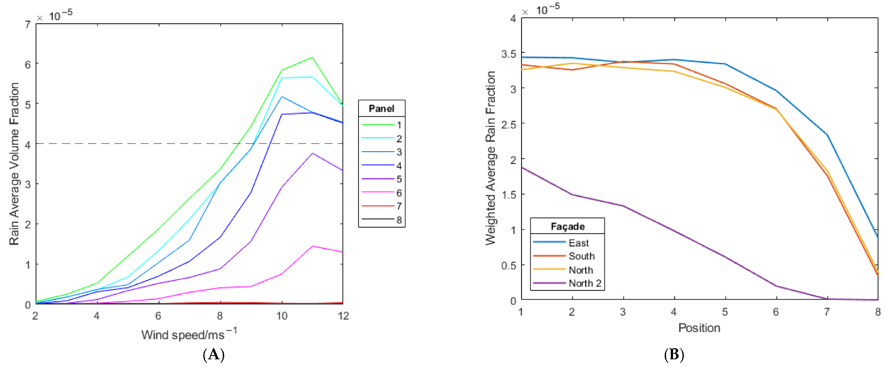
Figure 32.
Wind-speed probability distribution used (left) to calculate wind-speed weighted averaged rain fraction for each panel on each façade (right).
Figure 32.
Wind-speed probability distribution used (left) to calculate wind-speed weighted averaged rain fraction for each panel on each façade (right).
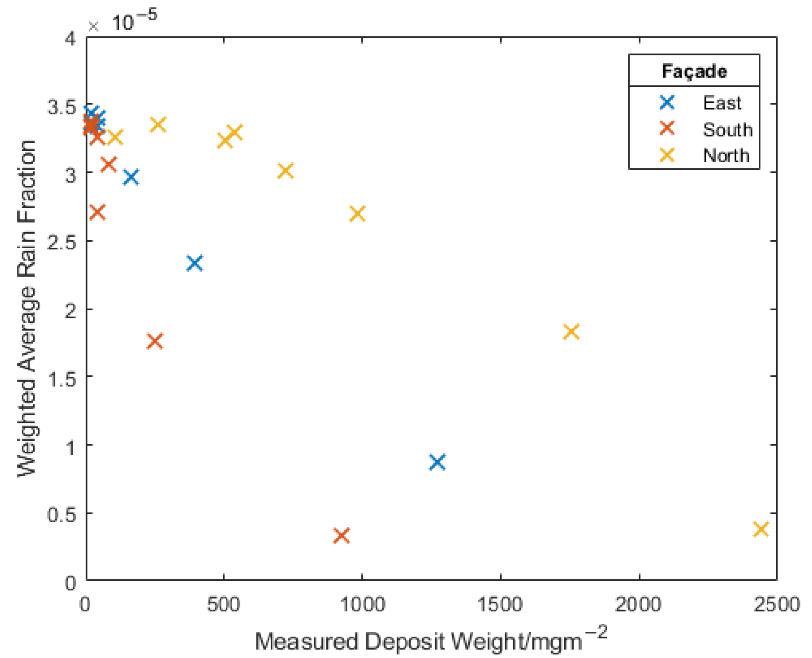
Figure 33.
Comparison between measured deposit fouling intensity and model predicted rain impact density.
Figure 33.
Comparison between measured deposit fouling intensity and model predicted rain impact density.
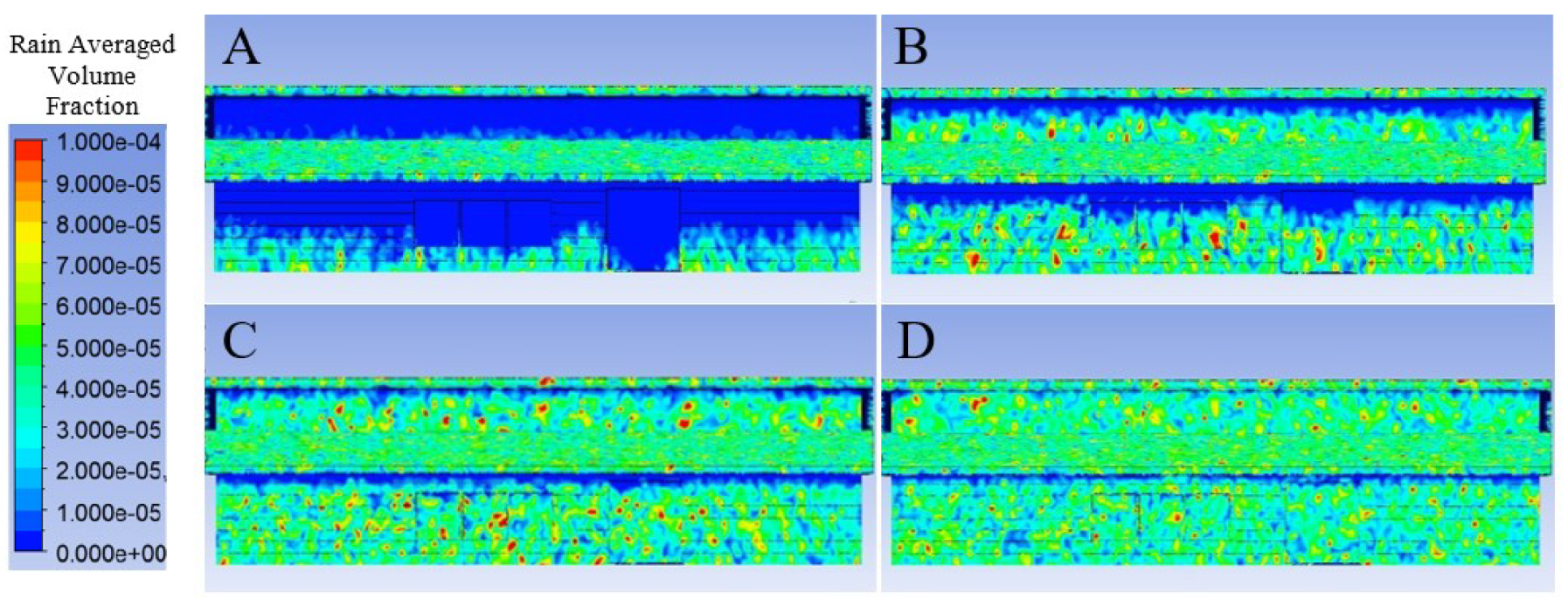
Figure 34.
Effect of the semi-shielding building on the predicted rain impact density for the north elevation under 2 (A), 4 (B), 6 (C), and 8 (D) ms−1 wind speed applied normal to the north elevation.
Figure 34.
Effect of the semi-shielding building on the predicted rain impact density for the north elevation under 2 (A), 4 (B), 6 (C), and 8 (D) ms−1 wind speed applied normal to the north elevation.
Figure 35.
(A) Measured average rain volume fraction at each location for the north façade in the dual building model. The dashed line represents the maximum volume fraction achieved in the single building model. (B) Comparison between the wind-speed-weighted rain impact density for the two models used.
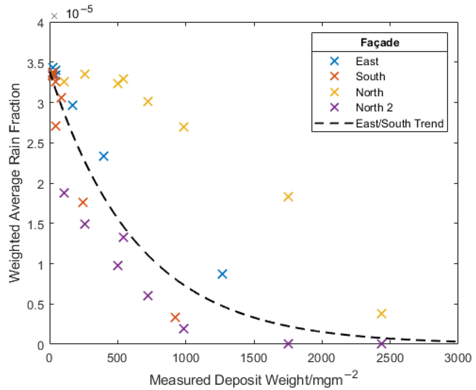
Figure 36.
Comparison of the fitting of north façade data from each model to the trend given by the east and south façade data.
Figure 36.
Comparison of the fitting of north façade data from each model to the trend given by the east and south façade data.
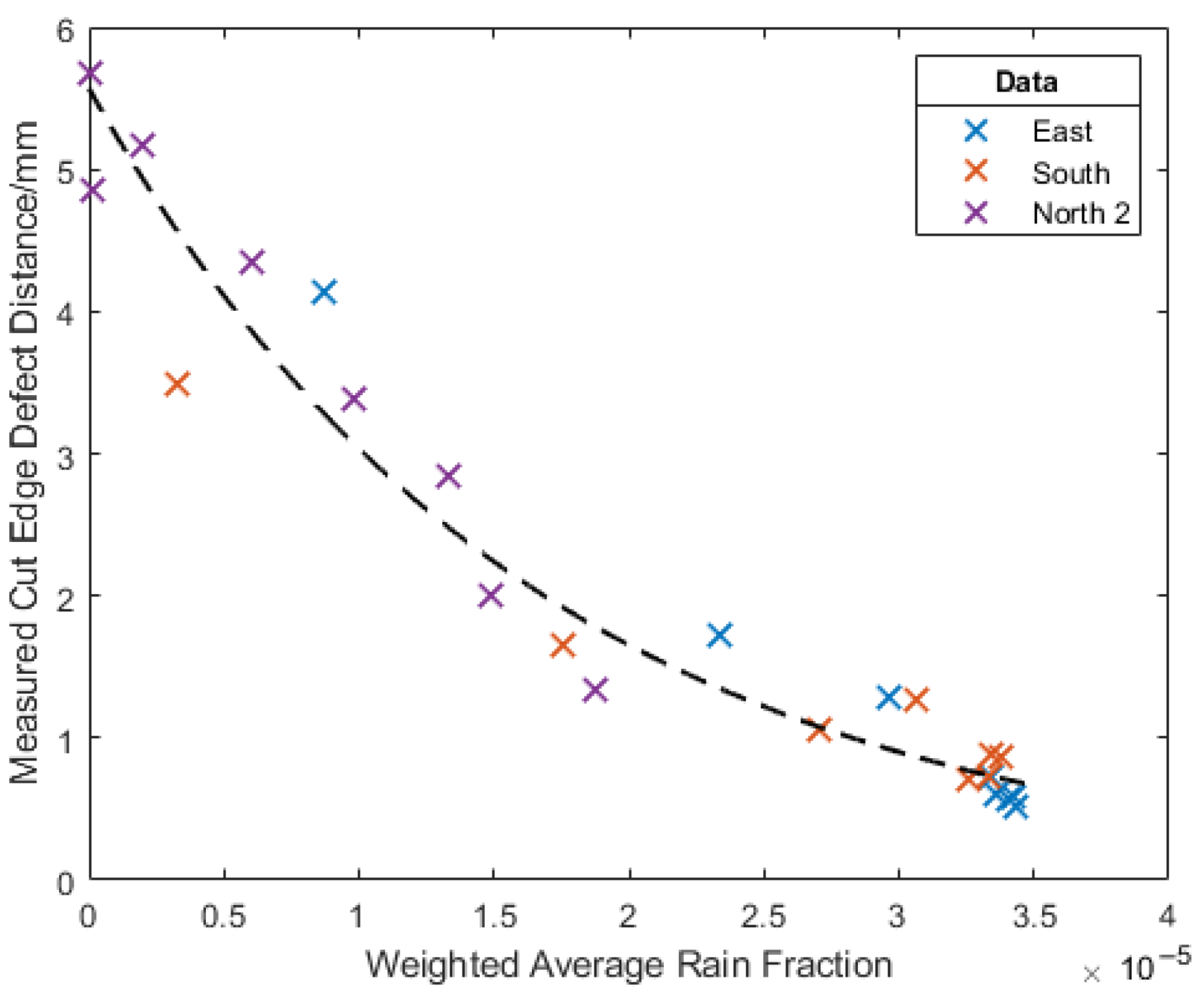
Figure 37.
Comparison of measured cut edge defect distance and the model-predicted rain impact density.
Figure 37.
Comparison of measured cut edge defect distance and the model-predicted rain impact density.
Table 1.
Building material characteristics.
Table 1.
Building material characteristics.
| Structure | Material |
|---|
| Roof | Standing seam profile integrated PV and coated steel roofing |
| Main structure | SIPS panels attached to steel frame |
| External cladding (walls) | Interlocking plank profile PVDF-coated steel panels, attached via rail system |
| Cladding (soffit, guttering) | PVC-coated steel |
| Windows and doors | Glass and aluminium construction |
Table 2.
Average weather data for this location.
Table 2.
Average weather data for this location.
| Metric | Location |
|---|
| Average temperature/°C | 4.4–16.8 |
| Average daily rainfall/mm | 3 |
| Average wind speed/ms−1 | 4.8–7.3 |
| Wind rose | ![Buildings 13 00270 i001]() |
| Average relative humidity/% | 81 |
| Average monthly sunlight/h | 50–210 |
Table 3.
Sensors used in the multifunctional sensing device.
Table 3.
Sensors used in the multifunctional sensing device.
| Parameter | Sensor | Operational Principle | Quoted Repeatability |
|---|
| Air temperature | Adafruit BME 680 | Diode Voltage | ±1 °C [28] |
| Humidity | Adafruit BME 680 | Capacitive | ±3% [28] |
| Panel temperature | Adafruit TMP 006 | IR Thermopile | ±1 °C [29] |
| UVA | Adafruit VEML 6075 | Photodiode | ±3 µWcm−1 [30] |
| UVB | Adafruit VEML 6075 | Photodiode | ±3 µWcm−1 [30] |
| Particulate concentration | Grove PPD42NS | Low Pulse Occupancy | ±50% [31] |
| Time of wetness | Grove Capacitive Moisture Sensor | Capacitive | ±5% |
Table 4.
Sensing box locations and their properties.
Table 4.
Sensing box locations and their properties.
| Number | Façade | Height | Location Type |
|---|
| 1 | South | Middle | Exposed |
| 2 | South | High | Sheltered by roof overhang |
| 3 | North | Low | Exposed/semi-sheltered by 2nd building |
| 4 | North | Middle | Exposed/semi-sheltered by 2nd building |
| 5 | North | High | Sheltered by roof overhang/semi-sheltered by 2nd building |
Table 5.
Simulation scenarios.
Table 5.
Simulation scenarios.
| Scenario | Model Used | Wind Direction | Wind Speeds Used ms−1 |
|---|
| 1–11 | Single building | From east | 2,3,4,5,6,7,8,9,10,11,12 |
| 12–22 | Single building | From south | 2,3,4,5,6,7,8,9,10,11,12 |
| 23–33 | Single building | From north | 2,3,4,5,6,7,8,9,10,11,12 |
| 34–44 | Dual building | From north | 2,3,4,5,6,7,8,9,10,11,12 |
Table 6.
Identified compounds and their likely sources.
Table 6.
Identified compounds and their likely sources.
| Filtered Sample (P) |
|---|
| Compound | Common Name | Found in/Possible Source |
|---|
| SiO2 | Silicon dioxide/silica | Sand |
| Fe2O3 | Iron (III) oxide | Corrosion product |
| NaCl | Sodium chloride/‘salt’ | Natural salt |
| CaCO3 | Calcium carbonate | Natural salt |
| Al2O3 | Aluminium oxide | Corrosion product |
| Unfiltered Sample (SP) |
| SiO2 | Silicon dioxide/silica | Sand |
| CaH4O6S | Calcium sulphate dihydrate | Gypsum building materials |
| Fe2O3 | Iron oxide | Corrosion product |
| NaCl | Sodium chloride/‘salt’ | Natural salt |
| CaCO3 | Calcium carbonate | Natural salt |
| Al2O3 | Aluminium oxide | Corrosion product |
Table 7.
Measured conductivity of different electrolytes.
Table 7.
Measured conductivity of different electrolytes.
| Sample | Measured Conductivity S/m |
|---|
| Deionised Water | 0.00 |
| 1 wt.% NaCl | 2.27 |
| 1 wt.% deposit | 1.65 |
| 5 wt.% NaCl | 2.75 |
| 5 wt.% deposit | 1.89 |
| Tap water | 0.10 |
| Rainwater | 0.10 |


