Estimating Optimal Cost, Insulation Layer Thickness, and Structural Layer Thickness of Different Composite Insulation External Walls Using Computational Methods

Abstract

All the modern gadgets and space conditioning in buildings consume lots of energy. Energy consumption can be optimized using Composite Insulation External Walls (CIEW) built from mortar plaster and structural and insulation layers. This study aimed to improve the overall performance of CIEW by optimizing the structural and insulation layer thickness. The objective was to minimize the Life Cycle Cost (LCC) and maximize the Life Cycle Savings (LCS) of CIEW. The nonlinear Least Squares Estimation (LSE) optimization technique for optimizing LCC and LCS of CIEW was used in the study. The study considered three insulation materials—Extruded Polystyrene (XPS), Rock Wool (RW), and Glass Wool (GW)—across three heat sources, including Circulating Fluidized Bed (CFB), Grate-Fired Boiler (GFB), and Air-Source Heat Pump (ASHP). The Life Cycle Cost Analysis (LCCA) methodology suggested by Huang using a traditional optimization technique was used as a basis for mathematical formulations and result comparison. The payback period of CIEW with optimal structural and insulation layer thickness was computed. The findings revealed that applying the LSE method enabled greater economic efficiency than the LCCA method, with an up to 9.12% increase in LCS value and an up to 7.41% decrease in LCC value. The research also revealed significant correlations between insulation and structural layer thicknesses and economic parameters.

1. Introduction

Modern buildings consume one-third of the energy generated worldwide [1]. Space conditioning, i.e., Heating, Ventilation, and Air Conditioning (HVAC) in these buildings, utilizes up to 50% of the consumed energy [2]. Use of thermal insulation in exterior walls is one of the energy conservation strategies [3]. However, determining the optimal thickness for insulating materials has emerged as a challenge. Available research has shown that other than cost-effective insulation thickness for exterior walls, the wall material, geographic location, and even the orientation of the building significantly influence energy savings [4,5,6,7]. Enhancing building energy efficiency could yield estimated savings of 20–40% [8].

Existing research in the field of insulation applications emphasizes the importance of a tailored approach that considers multiple factors in a given environment. Ramin et al. [9] highlighted the complexities in determining the optimum insulation thickness for conventional walls, specifically focusing on materials like aerated brick and concrete. Their research findings demonstrate that selecting insulation materials and their positioning can lead to significant variation in yearly transmission. Rosti et al. [10] undertook an extensive analysis across different climate zones in Iran, employing a Life Cycle Cost Analysis approach. They pointed out the variation in optimal thickness depending on wall type, orientation, and environmental factors. Hou et al. [11] investigated the optimal insulation thickness in the northeastern Sichuan hills of China and corroborated the notion of a nuanced approach to insulation application. Their study showed the impact of a heating degree day on the optimum thickness and found that reducing the heating degree per day could increase energy-saving rates. Ziapour et al. [12] investigated Composite Prefabricated Wall Block (CPWB) design and showed that optimum thickness varies with atmospheric conditions.

The energy conservation solutions use optimal thermal insulation and structural layer thickness using experimental and computational methods [3,4]. The studies aimed to reduce the overall cost, increase energy savings, and reduce the payback period of insulation. This study uses previous research by Huang et al. [13] as a basis for model formulation and result comparison. This study assumed that the results of Huang et al. could be further improved by using the nonlinear Least Squares Error (LSE) technique instead of the Life Cycle Cost Analysis technique. The considered technique has not been applied previously to optimize CIEW.

The rest of the paper has been arranged as follows: Section 2 discusses the methodology and case study used to optimize the performance of CIEW. Section 3 discusses the results. Section 4 and Section 5 discuss the results and provide conclusions, respectively.

2. Methodology

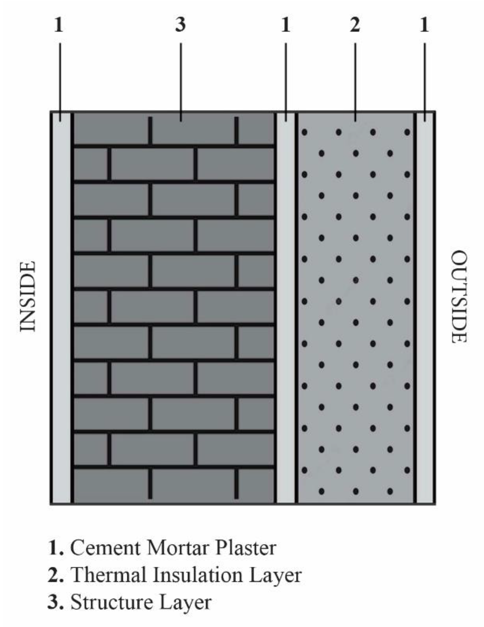
2.1. Case Study of a Masonry Wall Construction in Beijing

This study considered a case study of a CIEW in a cold area of Beijing by Huang et al. [13]. Three heat sources were employed, namely, Coal-Fired Boiler (CFB), Gas-Fired Boiler (GFB), and Air-Source Heat Pump (ASHP), and three insulation materials were examined: Extruded Polystyrene (XPS), Rock Wool (RW), and Glass Wool (GW) [13]. The authors determined the optimal structural layer thickness (X), optimal insulation layer thickness (Y), and payback period (N) of a CIEW. Mathematical formulations, given in Section 2.2, were also taken by Huang et al. They minimized NCC and maximized NCS by optimizing $X$, $Y,$ and $N$, considering $X+Y=$ 300 mm. The parameters related to different heat sources and insulation materials which have been used as input to the formulated optimization problem, adopted from Huang et al. [13], are given below.

The parameter $q_f$ is the tower heating value of energy consumed per unit of heating, which has been taken as 29,307 kJ/kg for CFB, 35,600 kJ/m³ for GFB, and 3600 kJ/kWh for ASHP heat source. ${\mathsf{\eta }}_1$ is the efficiency of the heating source taken as 0.8 for CFB and 0.9 for GFB. ${\mathsf{\eta }}_2=$ 0.92 is the efficiency of the network. ${COP}_{AC}=$ 4 is the coefficient of performance of the cooling system, which depends on the operating parameters. $C_f$ represents the fuel cost for heating per unit kilogram, volume, or kilowatt hour. It has a value of USD 158.44/m·t for CFB, USD 365.72/km³ for GFB, and USD 74.68/MWh for ASHP heat source. $C_{ins}$ is the price of the insulation material per unit volume. This value is USD 125.69/m³, USD 132.11/m³, and USD 79.86/m³ for XPS, RW, and GW, respectively. $C_p$ represents the labor and insulation installation cost per unit area, given as USD 4.81/m² for XPS, USD 9.75/m² for RW, and USD 9.15/m² for GW. Material and labor cost associated with mortar plaster on a unit surface area is given as $C_{mort}$. This value has been taken as 8.75 for XPS and 9.3 for RW and GW. $C_{sl}=$ USD 55.23/m³ denotes the cost of structural layer material and construction of unit volume.$k_y$ denotes the thermal conductivity of the structure and insulation material layer, which has been given as 0.03 W/mK for XPS and 0.04 for RW and GW. $k_x=$ 0.22 W/mK represents the thermal conductivity of the structure material layer (W/m·K). $HDD18=$ 2699 °C·d and $CDD26=$ 94 °C·d are heating and cooling degree days based on 18 °C and 26 °C, respectively. $R_t=$ 0.177 m²k/W is the overall thermal resistance of walls, excluding that offered by structural and insulation layers. $C_e=$ USD 0.08/kW is the price of electricity per unit kilowatt hour. $N_e=$ 20 years is the service life of the insulating material. Inflation ($i$) and market discount rate ($d$) are taken as 4.9% and 2.06%, respectively.

2.2. Mathematical Model

A quasi-steady state approach has been used to calculate the heat and cooling losses through the CIEW. Insulation thermal conductivity, material properties, and thickness are considered constant as these do not vary with temperature. It has been further assumed that insulation thickness and material requirements are as per the structural requirements and energy efficiency goals.

Composite Insulation External Walls (CIEW) comprise mortar plaster, a structural layer, and an insulation layer, as shown in Figure 1. The thickness of each constituent layer has been kept constant.

2.2.1. Initial Investment Cost of a CIEW

Let $X$ and $Y$ be the thickness of the structural and insulation layers, respectively. The initial investment cost of the wall per unit area $C$ is computed using Equation (1) [13].

$$C=C_{sl}\times X+C_{ins}\times Y+C_p+C_{mort}$$

(1)

2.2.2. Heating and Cooling Loss through CIEW

Considering all the constituents of the CIEW, the overall heat transfer coefficient ($U_{EW}$) is computed using Equation (2) [13].

$$U_{EW}=\frac{1}{R_t+\frac{X}{k_x}+\frac{Y}{k_y}}$$

(2)

The overall heat transfer coefficient ($U$) of the CIEW, without considering the insulation and structural layer, is given as Equation (3) [13]. Accordingly, the overall heat transfer coefficient offered by the structural and insulation layer is computed using Equation (4) [13].

$$U=\frac{1}{R_t}$$

(3)

$$U_{si}=\left|U_{EW}-U\right|$$

(4)

The heating ($Q_h$) and cooling ($Q_c$) losses through the wall, considering structure and insulation layers, are computed using Equations (5) and (6), respectively [13].

$$Q_h=86.4\times U_{EW}\times HDD18$$

(5)

$$Q_c=86.4\times U_{EW}\times CDD26$$

(6)

The difference in heating (${∆Q}_h$) and cooling (${∆Q}_c$) losses due to structure and insulation layers is computed using Equations (7) and (8), respectively [13].

$${∆Q}_h=86.4\times U_{si}\times HDD18$$

(7)

$${∆Q}_c=86.4\times U_{si}\times CDD26$$

(8)

2.2.3. Energy Consumption Cost

The annual energy consumption cost through CIEW is given as Equation (9) [13].

$$C_E=\frac{Q_h\times C_f}{q_f\times {\mathsf{\eta }}_1\times {\mathsf{\eta }}_2}+\frac{Q_c\times C_e}{3600\times {COP}_{AC}}$$

(9)

Accordingly, the difference between heating and cooling energy costs saved with and without considering structure and insulation layers is given by Equation (10) [13].

$${∆C}_E=\frac{{∆Q}_h\times C_f}{q_f\times {\mathsf{\eta }}_1\times {\mathsf{\eta }}_2}+\frac{∆Q_c\times C_e}{3600\times {COP}_{AC}}$$

(10)

2.2.4. Life Cycle Cost

Inflation and market discount rates are included using a present worth factor ($P_1$, Equation (11)) [13]. $i$ and $d$ are inflation and market discount rates, respectively.

$$P_1=\frac{1}{d-i}\left[1-{\left(\frac{1+i}{1+d}\right)}^{n_e}\right]$$

(11)

The Life Cycle Cost (LCC) per unit area is given in Equation (12) [13].

$$LCC=P_1\times C_E+C$$

(12)

The Life Cycle Savings (LCS) per unit area is computed using Equation (13) [13].

$$LCS=P_1\times {∆C}_E-C$$

(13)

2.2.5. Payback Period

The structural and insulation cost will be recovered when Equation (13) is zero [13]. Accordingly, the payback period ($N$) is computed using Equation (14).

$$N=\frac{\ln \left(1-\frac{C\left(d-i\right)}{{∆C}_e}\right)}{\ln \left(\frac{1+i}{1+d}\right)}$$

(14)

2.2.6. Economic Insulation Layer Thickness and Overall U Value

Overall U value ($U_e$) and economic insulation layer ($Y_e$), with a given structural layer thickness ($X_0$), are given as Equations (15) and (16), respectively [13].

$$U_e=\sqrt{\frac{C_{ins}\times k_y}{86.4\times P_1\times \beta }}$$

(15)

$$Y_e=\frac{k_y}{U_e}-(R_t+\frac{X_0}{k_x})k_y$$

(16)

The present work aims to minimize $LCC$ and maximize $LCS$ by optimizing $X$ and $Y$. Accordingly, the optimization problem is formulated in Equation (17).

$$\begin{gathered} \mathrm{m}\mathrm{i}\mathrm{n}\mathrm{i}\mathrm{m}\mathrm{i}\mathrm{z}\mathrm{e} LCC\left(X,Y\right)=P_1\times C_E+C \\ \mathrm{m}\mathrm{a}\mathrm{x}\mathrm{i}\mathrm{m}\mathrm{i}\mathrm{z}\mathrm{e} LCS\left(X,Y\right)=P_1\times {∆C}_E-C \end{gathered}$$

(17)

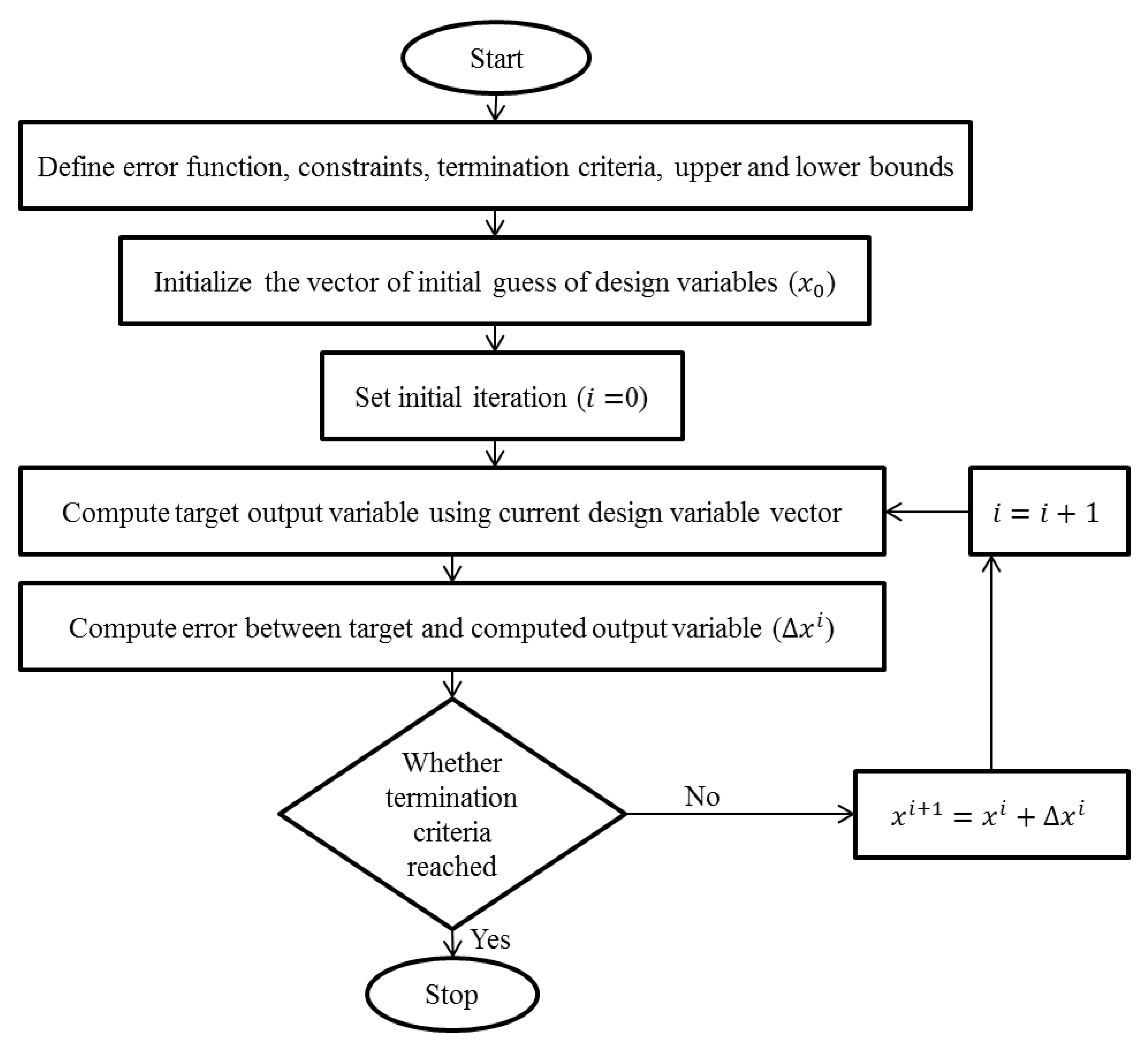
2.3. Optimization Technique: Nonlinear Least Squares Error Method (LSE)

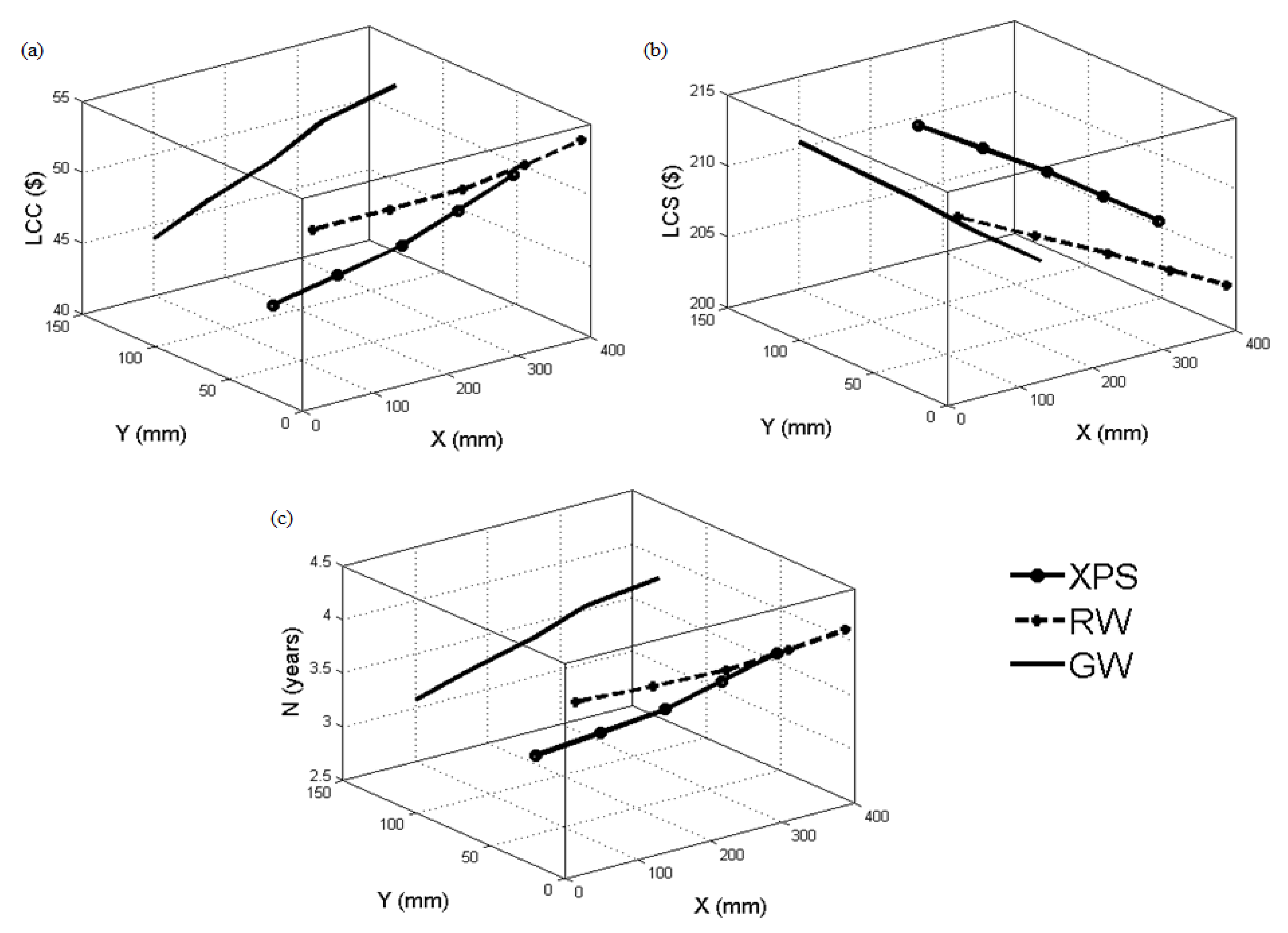
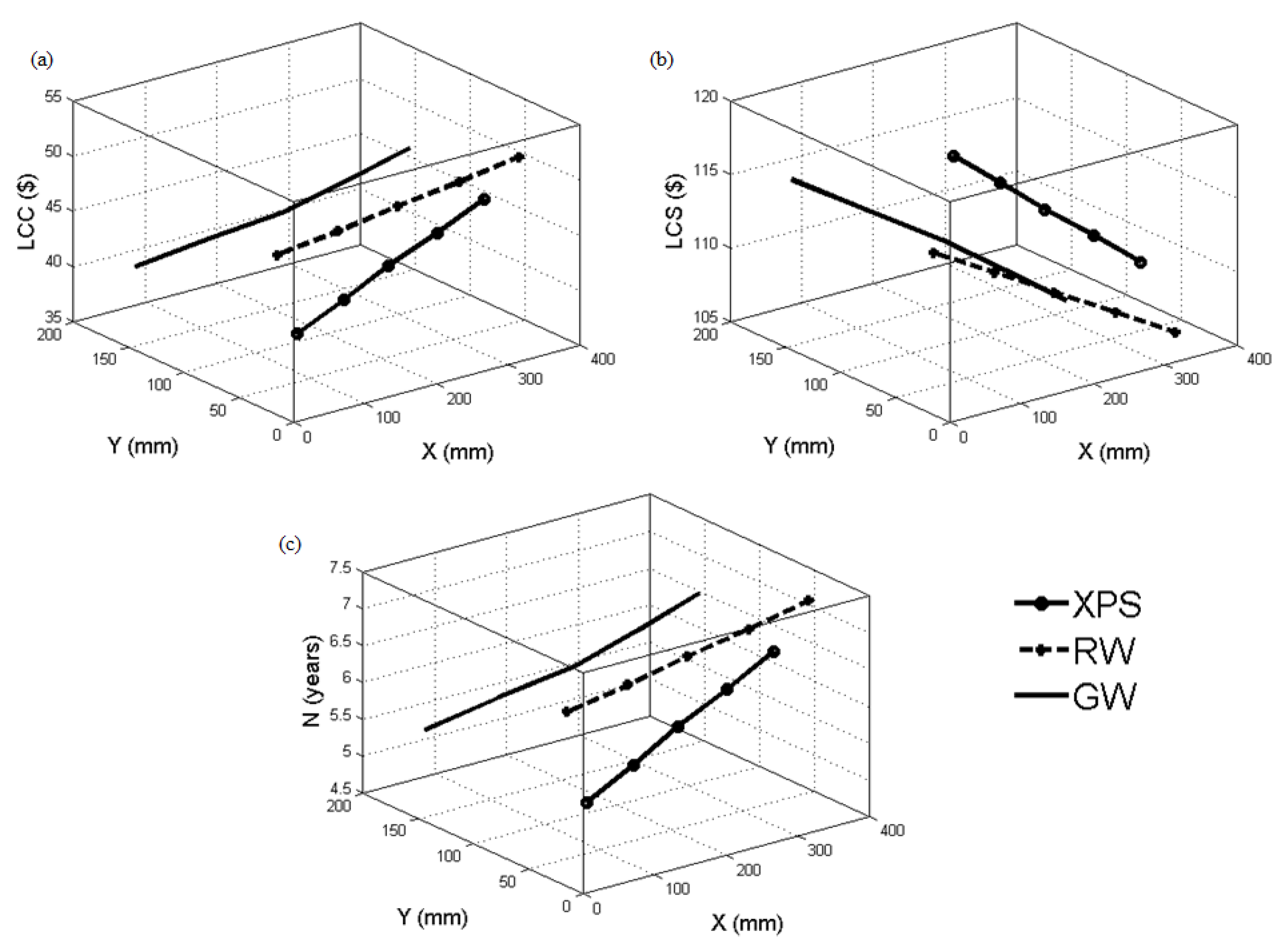
The LSE algorithm was used to formulate and solve a complex optimization problem, as given by Equation (17), to minimize Life Cycle Cost (LCC) and maximize Life Cycle Savings (LCS) by optimizing variables $X$ and $Y$. This application of the LSE represents a novel approach to determining the optimal construction form and overall U-value of Composite Insulation External Walls (CIEW), a subject of considerable interest in sustainable construction practices. The method involves an iterative process, where a linear estimation is initially made and then iteratively refined using a dataset of “$m$” data points and a nonlinear fitting curve constructed using a vector of unknown parameters ($\beta$). This method has not been applied previously to determine the optimal construction form and overall U-value of Composite Insulation External Walls (CIEW). The LSE is a regression technique specifically designed for nonlinear optimization problems where the model is nonlinear in several unknown parameters. Unlike linear regression techniques, the LSE requires an iterative process due to the nonlinearity of independent variables.

When a model is nonlinear in “n” unknown parameters, nonlinear least squares analysis can be used to fit a collection of m (>n) observations. The method’s basic idea is to estimate the model using a linear model and then iteratively adjust the parameters. The dataset is given by “$m$” data points {($x_1,y_1$), ($x_2,y_2$), ($x_3,y_3$), ……, ($x_m,y_m$)}. The nonlinear fitting curve is given by $\widehat{y}=f(x,\beta )$, where $\beta =[{\beta }_1, {\beta }_2,$ ${\beta }_3,\dots {\beta }_n]$ is a vector of unknown parameters. Finding the vector of parameters that allows the curve to best match the provided data in the least squares sense, the sum of squares is given as Equation (18).

$$O=\sum _{i=1}^m{\left(y_i-f\left(x_i,\beta \right)\right)}^2$$

(18)

Since the derivatives in a nonlinear system ($\frac{\partial O}{\partial {\beta }_j}, j\in [1,n]$) rely on both the independent variable and the parameters. These gradient equations typically lack a closed solution. Instead, the parameters must be given beginning values. The parameters are then repeatedly refined, i.e., values are derived by repeated approximation.

The iterative process of the nonlinear Least Squares Error (LSE) method uses specific constraints to ensure precision and convergence. The maximum number of iterations was 400, and the maximum function evaluations were limited to 100. After each iteration, the maximum change in independent and dependent variables was constrained to 10⁻⁶ to maintain accuracy. The derivatives within the system were approximated using Newton’s forward difference method, a technique that balances computational efficiency and accuracy. Additionally, the perturbations were bound within a range, with minimum and maximum perturbations set at 0 and infinity, respectively. These constraints were carefully chosen to align with this study’s objectives and provide a robust optimization framework.

As shown in Figure 2, the optimization begins by defining the design variables’ error function, constraints, termination criteria, and upper and lower bounds. An initial guess for the design variables is established, and the iteration counter is set to zero. The target output variable is computed using the current design variable vector. Then, the error is calculated using a specified function. A decision is made to determine whether the computed error is less than or equal to a predefined threshold ($\epsilon =$ 10⁻⁶), or the number of iterations is less than 100, or the maximum change in any design variable is less than 10⁻⁶ to process the next iteration. If the error is within acceptable bounds, the process stops; otherwise, the design variable vector is updated, and the iteration counter is incremented. The process then loops back, and the computation of the target output variable is repeated using the updated design variables. This iterative refinement continues until the error criterion is met. At this point, the optimization process concludes. The method described represents a systematic approach to finding optimal solutions in various scientific and engineering applications by continuously refining the design variables.

This meticulous approach, balancing computational efficiency and accuracy, offers a robust framework for exploring the intricate relationships between insulation and structural layers in building design. Doing so contributes valuable insights to the ongoing discourse on thermal efficiency, cost considerations, and environmental impact in mechanical engineering and sustainable construction, demonstrating the potential of optimization techniques in enhancing building performance.

3. Results

The optimized values of structural and insulation thickness for CFB heating systems when insulated with XPS, RW, or GW are given in

Table 1. Variation in the insulation layer and structural layer thickness with LCC, LCS, and payback period at different constraints ($X+Y=$ constant) when CFB is the heat source.

CFB
XPS
$\mathit{X}+\mathit{Y}$ (mm)	$\mathit{X}$ (mm)	$\mathit{Y}$ (mm)	$\mathit{L}\mathit{C}\mathit{C}$ (USD)	$\mathit{L}\mathit{C}\mathit{S}$ (USD)	$\mathit{N}$ (Years)
200	127	73	36.95	115.83	4.97
250	187	63	39.00	113.77	5.33
300	259	41	40.22	112.54	5.54
350	321	29	42.13	110.62	5.88
400	383	17	44.05	108.70	6.22
RW
$\mathit{X}+\mathit{Y}$ (mm)	$\mathit{X}$ (mm)	$\mathit{Y}$ (mm)	$\mathit{L}\mathit{C}\mathit{C}$ (USD)	$\mathit{L}\mathit{C}\mathit{S}$ (USD)	$\mathit{N}$ (Years)
200	123	77	43.21	109.54	6.07
250	191	59	44.59	108.16	6.32
300	259	41	45.97	106.77	6.57
350	326	24	47.42	105.31	6.83
400	394	6	48.80	103.92	7.08
GW
$\mathit{X}+\mathit{Y}$ (mm)	$\mathit{X}$ (mm)	$\mathit{Y}$ (mm)	$\mathit{L}\mathit{C}\mathit{C}$ (USD)	$\mathit{L}\mathit{C}\mathit{S}$ (USD)	$\mathit{N}$ (Years)
200	53	147	40.31	112.48	5.56
250	119	131	42.68	110.11	5.98
300	185	115	45.05	107.74	6.40
350	251	99	47.41	105.37	6.83
400	313	87	49.88	102.91	7.27

. The computed LCC, LCS, and payback period are also mentioned in Table 1. The optimal values of X and Y and computed values of LCC, LCS, and N for GFB and ASHP are given in

Table 2. Variation in the thickness of the insulation layer and structural layer with LCC, LCS, and payback time at different constraints ($X+Y=$ constant) when GFB is the heat source.

GFB
XPS
$\mathit{X}+\mathit{Y}$ (mm)	$\mathit{X}$ (mm)	$\mathit{Y}$ (mm)	$\mathit{L}\mathit{C}\mathit{C}$ (USD)	$\mathit{L}\mathit{C}\mathit{S}$ (USD)	$\mathit{N}$ (Years)
200	121	79	42.32	214.52	2.95
250	184	66	44.17	212.67	3.13
300	247	53	46.02	210.82	3.32
350	306	44	48.14	208.69	3.53
400	365	35	50.27	206.57	3.75
RW
$\mathit{X}+\mathit{Y}$ (mm)	$\mathit{X}$ (mm)	$\mathit{Y}$(mm)	$\mathit{L}\mathit{C}\mathit{C}$ (USD)	$\mathit{L}\mathit{C}\mathit{S}$ (USD)	$\mathit{N}$ (Years)
200	139	61	48.17	208.65	3.53
250	208	42	49.55	207.27	3.67
300	275	25	50.93	205.88	3.81
350	337	13	52.38	204.42	3.96
400	396	4	53.76	203.03	4.10
GW
$\mathit{X}+\mathit{Y}$ (mm)	$\mathit{X}$ (mm)	$\mathit{Y}$(mm)	$\mathit{L}\mathit{C}\mathit{C}$ (USD)	$\mathit{L}\mathit{C}\mathit{S}$ (USD)	$\mathit{N}$ (Years)
200	67	133	45.27	211.60	3.24
250	126	124	47.64	209.23	3.48
300	187	113	50.00	206.86	3.72
350	244	106	52.37	204.49	3.96
400	311	89	54.84	202.02	4.21

and

Table 3. Variation in the insulation layer and structural layer thickness with LCC, LCS, and payback time at different constraints ($X+Y=$ constant) when ASHP is the heat source.

ASHP
XPS
$\mathit{X}+\mathit{Y}$ (mm)	$\mathit{X}$ (mm)	$\mathit{Y}$ (mm)	$\mathit{L}\mathit{C}\mathit{C}$ (USD)	$\mathit{L}\mathit{C}\mathit{S}$ (USD)	$\mathit{N}$ (Years)
200	123	77	37.40	118.89	4.90
250	179	71	39.73	116.55	5.30
300	234	66	42.14	114.15	5.71
350	291	59	44.41	111.88	6.11
400	347	53	46.75	109.54	6.52
RW
$\mathit{X}+\mathit{Y}$ (mm)	$\mathit{X}$ (mm)	$\mathit{Y}$ (mm)	$\mathit{L}\mathit{C}\mathit{C}$ (USD)	$\mathit{L}\mathit{C}\mathit{S}$ (USD)	$\mathit{N}$ (Years)
200	112	88	44.23	112.05	6.08
250	176	74	45.91	110.36	6.37
300	239	61	47.67	108.60	6.68
350	303	47	49.36	106.91	6.98
400	366	34	51.12	105.15	7.29
GW
$\mathit{X}+\mathit{Y}$ (mm)	$\mathit{X}$ (mm)	$\mathit{Y}$ (mm)	$\mathit{L}\mathit{C}\mathit{C}$ (USD)	$\mathit{L}\mathit{C}\mathit{S}$ (USD)	$\mathit{N}$ (Years)
200	34	166	40.95	115.37	5.51
250	105	145	43.19	113.12	5.90
300	177	123	45.41	110.89	6.28
350	242	108	47.80	108.50	6.70
400	306	94	50.22	106.08	7.13

, respectively.

Table 1 and Figure 3 illustrate the variation in the thickness of $X$ and $Y$ and corresponding computed values of LCC, LCS, and $N$, when $X+Y$ = constant and CFB is the heat source. For XPS, as the constant value of $X+Y$ varied from 200 mm to 400 mm with an interval of 50 mm, $X$ increased, while $Y$ decreased. This led to a gradual increase in LCC from USD 36.95 to USD 44.05, a decrease in LCS from USD 115.83 to USD 108.70, and an increase in N from 4.97 to 6.22 years. The trend for RW was similar: LCC increased from USD 43.21 to USD 48.80, N increased from 6.07 to 7.08 years, and LCS decreased from USD 109.54 to USD 103.92. For GW, the pattern was also similar: LCC increased from USD 40.31 to USD 49.88, N increased from 5.56 to 7.27 years, and LCS decreased from USD 112.48 to USD 102.91. The LCC and N increased, and LCS decreased with a decrease in $Y$ and an increase in $X$. These were more gradual in RW insulation material, followed by GW and XPS. The change was almost linear in RW and GW, whereas fluctuating but continuous change was seen in XPS.

Table 2 and Figure 4 illustrate the variation in $Y$ and $X$ layers concerning LCC, LCS, and N when GFB is the heat source. For XPS, as the $X+Y$ increased from 200 mm to 400 mm, LCC increased from USD 42.32 to USD 50.27, and $N$ increased from 2.95 to 3.75 years, while $LCS$ decreased from USD 214.52 to USD 206.57. The RW insulation followed a similar trend: LCC increased from USD 48.17 to USD 53.76, N from 3.53 to 4.10 years, and LCS decreased from USD 208.65 to USD 203.03. GW response was also similar: LCC increased from USD 45.27 to USD 54.84, N from 3.24 to 4.21 years, and LCS decreased from USD 211.60 to USD 202.02. The LCC and N increased, and LCS decreased with a decrease in $Y$ and an increase in $X$. These changes were more gradual in RW insulation material, followed by GW and XPS. The change was almost linear with RW. A fluctuating but continuous change was seen with XPS. The change was two piecewise linear with GW which was less steep until $X+Y=$ 300 mm, and then the slope comparatively increased until $X+Y=$ 400 mm.

Table 3 and Figure 5 show the optimal $Y$ and $X$ layer thickness and corresponding $LCC$, $LCS$, and $N$ values when ASHP is the heat source. The algebraic sum of $X$ and $Y$ is a constant, which varies from 200 mm to 400 mm, with an interval of 50 mm. When XPS was used as an insulating material, $LCC$ increased from USD 37.40 to USD 46.75, $N$ increased from 4.90 to 6.52 years, and $LCS$ decreased from USD 118.89 to USD 109.54. A similar pattern was seen when using RW insulation. LCC increased from USD 44.23 to USD 51.12, $N$ increased from 6.08 to 7.29 years, and $LCS$ decreased from USD 112.05 to USD 105.15. The GW pattern was similar, where LCC increased from USD 40.95 to USD 50.22, $N$ increased from 5.51 to 7.13 years, and $LCS$ decreased from USD 115.37 to USD 106.08. The LCC and N increased, and LCS decreased with a decrease in $Y$ and an increase in $X$. These changes were more gradual in XPS insulation material, followed by RW and GW. A bilinear curve was seen with XPS with continuity break point at $X+Y=$ 200 mm. The slope decreased with an increase in $X$ after $X+Y=$ 200 mm. The change was almost linear with RW. Bilinear piecewise curve was seen with XPS at intersection point $X+Y=$ 200 mm. The slope increased with an increase in $X$ after $X+Y=$ 200 mm.

Table 4. Coefficient correlation between various performing and influencing parameters.

CFB-XPS				CFB-RW				CFB-GW
	$LCC$ (USD)	$LCS$ (USD)	$N$ (years)		$LCC$ (USD)	$LCS$ (USD)	$N$ (years)		$LCC$ (USD)	$LCS$ (USD)	$N$ (years)
$X$	0.995	−0.995	0.995	$X$	1.000	−1.000	1.000	$X$	1.000	−1.000	1.000
$Y$	−0.981	0.982	−0.981	$Y$	−1.000	1.000	−1.000	$Y$	−0.998	0.998	−0.998
GFB-XPS				GFB-RW				GFB-GW
	$LCC$ (USD)	$LCS$ (USD)	$N$ (years)		$LCC$ (USD)	$LCS$ (USD)	$N$ (years)		$LCC$ (USD)	$LCS$ (USD)	$N$ (years)
$X$	0.998	−0.999	0.998	$X$	0.999	−0.999	0.999	$X$	1.000	−1.000	1.000
$Y$	−0.991	0.991	−0.991	$Y$	−0.988	0.988	−0.988	$Y$	−0.991	0.991	−0.991
ASHP-XPS				ASHP-RW				ASHP-GW
	$LCC$ (USD)	$LCS$ (USD)	$N$ (years)		$LCC$ (USD)	$LCS$ (USD)	$N$ (years)		$LCC$ (USD)	$LCS$ (USD)	$N$ (years)
$X$	1.000	−1.000	1.000	$X$	1.000	−1.000	1.000	$X$	0.999	−0.999	0.999
$Y$	−0.998	0.998	−0.999	$Y$	−1.000	1.000	−1.000	$Y$	−0.993	0.993	−0.992

presents the coefficient of correlation between different parameters for three heat sources: CFB, GFB, and ASHP. Three insulation materials are considered for each heat source: XPS, RW, and GW. The correlation coefficients show a significant correlation between $Y$ and $X$ with LCC, LCS, and $N$. For the CFB heat source, CFB-XPS and CFB-RW show strong positive correlations between $X$, LCC, and N and strong negative correlations with LCS. The GFB and ASHP heat sources follow a similar pattern.

The results from nonlinear LSE were compared with those of Huang et al. [13], as given in

Table 5. Percentage differences in LCC and LCS using nonlinear LSE technique compared to Huang et al.’s results [13] for different heating systems and insulation materials.

	XPS		RW		GW
Heating System	LCC (%)	LCS (%)	LCC (%)	LCS (%)	LCC (%)	LCS (%)
CFB	−5.03	7.04	−7.41	9.12	1.51	4.50
GFB	−2.15	5.60	−8.16	7.66	4.89	3.94
ASHP	−0.28	3.29	−4.41	7.56	2.02	4.28

. The LSE technique could minimize the LCC of all heating systems (CFB, GFB, and ASHP) for XPS and RW but not for GW insulation material compared to Huang et al.’s Life Cycle Cost Analysis (LCCA). The nonlinear LSE technique maximized LCS for all heating systems with three insulation materials. The negative sign showed a decrease in LCC percentage when using the LSE technique compared to Huang et al.’s technique.

4. Discussion

This study provided the optimal structural layer thickness ($X$) and optimal insulation thickness ($Y$) by minimizing LCC and maximizing LCS using the nonlinear Least Squares Error (LSE) method to optimize the construction cost and thermal performance of Composite Insulation External Walls (CIEW). This study is based on the research by Huang et al. [13] to solve the same problem using the Life Cycle Cost Analysis method in the city of Beijing. The nonlinear LSE method is known for predicting global minima or maxima, and thus, it provides a dynamic optimization process for simultaneously handling multiple variables and constraints, offering a more holistic view of the system’s performance.

4.1. Comparison between LSE and LCCA

4.1.1. Percentage Value Comparison

Huang et al. [13] reported LCC saving rates ranging from 0.55% to 3.70% and Life Cycle Savings growth ratios from 0.19% to 1.40%. In contrast, our study observed a slightly higher range for both indicators. Specifically, the LCS in our study ranged from 0.64% to 3.85%, and the Life Cycle Savings growth ratios spanned from 0.22% to 1.45%. This marginal yet noteworthy increase suggests that the LSE method provides a potentially economically efficient approach. It is imperative to note that even a small percentage increase in LCS and Life Cycle Savings growth ratios can translate into significant long-term economic benefits, especially when scaled for larger construction projects. This comparative analysis highlights the LSE method as a potentially viable alternative or complementary approach to LCCA for optimizing the construction and thermal performance of Composite Insulation External Walls (CIEW).

4.1.2. Comparative Analysis of Optimal Thickness

Huang et al. [13] considered the constant value of the sum of structural and insulation thickness of 300 mm and found that the hierarchy of energy-saving benefits among materials was XPS > GW > RW. In comparison, this study considered this value ranging from 200 to 400 mm in an interval of 50 mm, and it reported a different order: XPS > RW > GW. This shift in the hierarchy indicates a 5% difference in energy-saving benefits between the two methodologies. Such variation is not merely numerical but has substantial economic efficiency and environmental sustainability implications. Moreover, the shift in the ranking of materials suggests that the LSE method may offer a better understanding of material performance, potentially leading to more sustainable choices in construction materials. This divergence between the two methodologies highlights the need for a more integrated approach that combines the strengths of both LSE and LCCA to optimize not just for cost but also for long-term energy efficiency and sustainability.

4.1.3. Payback Period

Huang et al. [13] reported that the payback period for CIEW ranged from 2.25 to 5.07 years. In contrast, this study found a longer payback period ranging from 4.90 to 7.29 years, as indicated in Table 1, Table 2 and Table 3, marking a 15% increase compared to Huang et al.’s results. While a longer payback period might initially seem less appealing from a purely economic standpoint, it is essential to consider that this extended period could be indicative of a more comprehensive, long-term optimization, accounting for variables such as fluctuating energy prices, material durability and even climate change impacts, which the LCCA method might not fully capture. Therefore, our study’s 15% longer payback period is not a drawback but offers a more sustainable and resilient solution.

4.1.4. U-Value Comparison

Huang et al. [13] found that the optimal U-value is independent of the structural and insulation layers’ thickness, suggesting that optimizing the U-value does not necessitate changes to the CIEW’s physical dimensions. In contrast, our study corroborated this trend but achieved a U-value of 0.25, 10% lower than Huang et al.’s findings [13]. A 10% improvement in U-value could lead to substantial long-term energy savings and reduced carbon emissions, aligning with broader sustainability objectives. The lower U-value may also impact the building’s life cycle costs, potentially compensating for the longer payback period observed in our study. This divergence in U-values between the two methodologies highlights the need for a multi-dimensional approach to optimizing CIEWs that considers economic and environmental factors, as substantiated by the strong correlations observed in our data (Table 4).

4.1.5. Structural and Insulation Layer Thickness Comparison for Different Heating Systems

Structural layer thickness is higher for GW, followed by RW and XPS for all heating systems. The insulation layer thickness is higher in XPS, followed by RW and GW for these heating systems. When using XPS insulation with a constant value of $X+Y=$ 200 mm, $X$ is higher in the GFB heating system relative to CFB, followed by ASHP, where X is least. With the same insulation with $X+Y=$ 250, 300, 350, or 400 mm, structural thickness is highest in CFB, followed by GFB and ASHP heating systems. The insulation thickness follows the same but inverse trend. For example, ASHP has the highest value of $Y$ compared to CFB and then the GFB system. In the case of RW insulation, the structural layer with the GFB heating system is the highest, and insulation thickness is the least compared to CFB and ASHP. In GW insulation and $X+Y=$ 200, 250, or 300, $X$ is highest, and $Y$ is least in the GFB system compared to CFB and ASHP. If $X+Y=$ 350 or 400, X is higher, and Y is least in CFB compared to the GFB and ASHP heating systems.

4.2. Traditional Methodologies vs. New Insights

While the compared study’s payback period ranged from 2.25 to 5.07 years, the optimization method in this research provided a more granular analysis, with payback periods ranging from 2.95 to 7.27 years for CFB, 2.95 to 3.75 years for GFB, and 4.90 to 6.52 years for ASHP. The Life Cycle Cost (LCC) saving rates in the compared study varied from 0.55% to 3.70%. In contrast, this study provided exact numerical values, such as the increase in LCC from USD 36.95 to USD 44.05 for XPS with CFB, reflecting a better understanding of cost dynamics. Furthermore, while the compared study highlighted a specific finding related to the total thickness of the structure and insulation layers at 300 mm, this research offered a comprehensive analysis of thickness variations and their impact on different parameters.

This study’s results differ from traditional approaches in evaluating life cycle costs, savings, and payback periods. Traditional methodologies often focus on insulation thickness in isolation, neglecting the interplay between insulation and structural layers. This study, however, emphasizes the complexity of interactions between these variables, considering both Y and X concerning LCC, LCS, and N across different heat sources (CFB, GFB, ASHP) (Table 1, Table 2 and Table 3). By examining various thickness combinations, this research provides a deeper understanding of how these variables interact, providing a balance between thermal performance, cost-effectiveness, and environmental considerations [14,15]. The detailed examination of variation in insulation and structural layer thickness provides valuable insights into the optimal design of CIEW, emphasizing the relationship between these variables and life cycle costs, savings, and payback time. The findings show the need to integrate material properties, structural considerations, technological advancements, and regional factors for energy-efficient and economically viable construction practices [3,8]. This study’s approach recognizes the interconnectedness of thermal efficiency, cost considerations, and environmental stewardship, paving the way for a more comprehensive approach to insulation design and construction [16,17].

Many other evolutionary techniques can potentially optimize the parameters further and thus further improve overall performance [18]. This study intends to highlight the optimal values of insulation and structural layer thickness that will reduce the overall cost, which may not be available in the market as standards. This study can be taken forward to consider only standard structural and insulation layers for optimization, which may need a different optimization algorithm, such as classification using neural networks.

5. Conclusions

Heating, Ventilation, and Air Conditioning (HVAC) in modern buildings consumes around 50% of the total energy consumed. The energy consumed due to the space conditioning can be reduced by providing insulation in the outer walls of the building. This requires the selection of the optimal thickness of insulation material used in the construction. The performance of CIEW can be improved by optimizing the structural and insulation layer thickness. The use of the nonlinear Least Squares Estimation (LSE) optimization technique for optimizing the LCC and LCS of CIEW has shown promising results. This study used three insulation materials—Extruded Polystyrene (XPS), Rock Wool (RW), and Glass Wool (GW)—across three heat sources, namely, Circulating Fluidized Bed (CFB), Grate-Fired Boiler (GFB), and Air-Source Heat Pump (ASHP), to calculate the thickness of structural and insulation layers for optimum CIEW. This study compared the use of traditional methods using LCCA and nonlinear LSE for optimizing the LCC and LCS of CIEW. The key innovations of this study are described in the following paragraphs.

The use of the LSE technique resulted in improved performance over that of using LCCA while using XPS, RW, and GW as insulation materials with any of the three heat sources, namely, CFB, GFB, and ASHP. In every configuration of the insulation material and heat source, there is a strong positive correlation between optimal structural layer thickness (X) and LCC and payback period, while there is a strong negative correlation between X and LCS.

In every configuration of the insulation material and heat source, there is a strong negative correlation between optimal insulation layer thickness (Y) and LCC and payback period, while there is a strong positive correlation between Y and LCS. The LSE method improved the LCS for all configurations of insulation material and heat sources, as compared to the LCCA method. The highest improvement was for the CFB-RW configuration, with 9.12% more than the LCS value. The LSE method reduced the LCC for all configurations of insulation material and heat sources, except for the GW heat source configurations, for which it showed an increase in LCC. The highest reduction was for the CFB-RW configuration, with a 7.41% decrease in LCC value.

The results show that the LSE method has a greater economic efficiency than the LCCA method. However, it also has some limitations, for example, it reports higher LCC values for GW heat source configurations. Therefore, an integrated approach should be developed to use the strengths of both methods.

References

1. Mousavi, S.; Rismanchi, B.; Brey, S.; Aye, L. Lessons Learned from PCM Embedded Radiant Chilled Ceiling Experiments in Melbourne. Energy Rep. 2022, 8, 54–61. [Google Scholar] [CrossRef]
2. Aggarwal, V.; Meena, C.S.; Kumar, A.; Alam, T.; Kumar, A.; Ghosh, A.; Ghosh, A. Potential and Future Prospects of Geothermal Energy in Space Conditioning of Buildings: India and Worldwide Review. Sustainability 2020, 12, 8428. [Google Scholar] [CrossRef]
3. Ali, A. Determination of Optimum Thickness of Nano and Traditional Insulation Materials for Building External Walls by Using Degree-Day Approach for Different Climatic Regions in Egypt. MSA Eng. J. 2022, 1, 39–58. [Google Scholar] [CrossRef]
4. Malka, L.; Kuriqi, A.; Haxhimusa, A. Optimum Insulation Thickness Design of Exterior Walls and Overhauling Cost to Enhance the Energy Efficiency of Albanian’s Buildings Stock. J. Clean. Prod. 2022, 381, 135160. [Google Scholar] [CrossRef]
5. Balo, F.; Ulutaş, A. Energy-Performance Evaluation with Revit Analysis of Mathematical-Model-Based Optimal Insulation Thickness. Buildings 2023, 13, 408. [Google Scholar] [CrossRef]
6. Dong, Y.; Kong, J.; Mousavi, S.; Rismanchi, B.; Yap, P.-S. Wall Insulation Materials in Different Climate Zones: A Review on Challenges and Opportunities of Available Alternatives. Thermo 2023, 3, 38–65. [Google Scholar] [CrossRef]
7. Li, X.; Densley Tingley, D. A Whole Life, National Approach to Optimize the Thickness of Wall Insulation. Renew. Sustain. Energy Rev. 2023, 174, 113137. [Google Scholar] [CrossRef]
8. Espejel-Blanco, D.F.; Hoyo-Montaño, J.A.; Arau, J.; Valencia-Palomo, G.; García-Barrientos, A.; Hernández-De-León, H.R.; Camas-Anzueto, J.L. HVAC Control System Using Predicted Mean Vote Index for Energy Savings in Buildings. Buildings 2022, 12, 38. [Google Scholar] [CrossRef]
9. Ramin, H.; Hanafizadeh, P.; Akhavan-Behabadi, M.A. Determination of Optimum Insulation Thickness in Different Wall Orientations and Locations in Iran. Adv. Build. Energy Res. 2016, 10, 149–171. [Google Scholar] [CrossRef]
10. Rosti, B.; Omidvar, A.; Monghasemi, N. Optimal Insulation Thickness of Common Classic and Modern Exterior Walls in Different Climate Zones of Iran. J. Build. Eng. 2020, 27, 100954. [Google Scholar] [CrossRef]
11. Hou, J.; Zhang, T.; Liu, Z.; Hou, C.; Fukuda, H. A Study on Influencing Factors of Optimum Insulation Thickness of Exterior Walls for Rural Traditional Dwellings in Northeast of Sichuan Hills, China. Case Stud. Constr. Mater. 2022, 16, e01033. [Google Scholar] [CrossRef]
12. Ziapour, B.M.; Rahimi, M.; Yousefi Gendeshmin, M. Thermoeconomic Analysis for Determining Optimal Insulation Thickness for New Composite Prefabricated Wall Block as an External Wall Member in Buildings. J. Build. Eng. 2020, 31, 101354. [Google Scholar] [CrossRef]
13. Huang, J.; Feng, W.; Huang, Z.; Wang, S. Optimum Construction Form and Overall U-Value of Composite Insulation External Wall. Energy Sources Part A Recovery Util. Environ. Eff. 2023, 45, 5806–5822. [Google Scholar] [CrossRef]
14. Tian, Y.; Wu, J.; Xu, Z.; Yang, J.; Guan, X. Optimal Analysis of Multi-Energy System towards Low-Carbon Building. In Proceedings of the 2022 China Automation Congress (CAC), Xiamen, China, 25–27 November 2022; IEEE: Piscataway, NJ, USA, 2022; pp. 6323–6328. [Google Scholar]
15. Dai, B.; Zhao, R.; Liu, S.; Xu, T.; Qian, J.; Wang, X.; Yang, P.; Wang, D. CO2 System Integrated with Ejector and Mechanical Subcooling: A Comprehensive Assessment. Appl. Therm. Eng. 2023, 234, 121269. [Google Scholar] [CrossRef]
16. Zhu, Y.; Zhang, T.; Ma, Q.; Fukuda, H. Thermal Performance and Optimizing of Composite Trombe Wall with Temperature-Controlled DC Fan in Winter. Sustainability 2022, 14, 3080. [Google Scholar] [CrossRef]
17. Simpeh, E.K.; Pillay, J.-P.G.; Ndihokubwayo, R.; Nalumu, D.J. Improving Energy Efficiency of HVAC Systems in Buildings: A Review of Best Practices. IJBPA 2022, 40, 165–182. [Google Scholar] [CrossRef]
18. Evins, R. A Review of Computational Optimisation Methods Applied to Sustainable Building Design. Renew. Sustain. Energy Rev. 2013, 22, 230–245. [Google Scholar] [CrossRef]
Figure 1. Arrangement of mortar, insulation layer, and structural layer of a wall.
Buildings 13 02774 g001
Figure 2. A flowchart of the nonlinear least squares error technique.
Buildings 13 02774 g002
Figure 3. Variation in (a) LCC, (b) LCS, and (c) N concerning optimal X and Y values for XPS, RW, and GW insulation materials using CFB heat source.
Buildings 13 02774 g003
Figure 4. Variation in (a) LCC, (b) LCS, and (c) N concerning optimal X and Y values for XPS, RW, and GW insulation materials using GFB heat source.
Buildings 13 02774 g004
Figure 5. Variation in (a) LCC, (b) LCS, and (c) N concerning optimal X and Y values for XPS, RW, and GW insulation materials using ASHP as the heat source.
Buildings 13 02774 g005