A Comparative Analysis of Slope Failure Prediction Using a Statistical and Machine Learning Approach on Displacement Data: Introducing a Tailored Performance Metric

Abstract

Slope failures pose significant threats to human safety and vital infrastructure. The urgent need for the accurate prediction of these geotechnical events is driven by two main goals: advancing our understanding of the underlying geophysical mechanisms and establishing efficient evacuation protocols. Although traditional physics-based models offer in-depth insights, their reliance on numerous assumptions and parameters limits their practical usability. In our study, we constructed an experimental artificial slope and monitored it until failure, generating an in-depth displacement dataset. Leveraging this dataset, we developed and compared prediction models rooted in both statistical and machine learning paradigms. Furthermore, to bridge the gap between generic evaluation metrics and the specific needs of slope failure prediction, we introduced a bespoke performance. Our results indicate that while the statistical approach did not effectively provide early warnings, the machine learning models, when assessed with our bespoke performance metric, showed significant promise as reliable early warning systems. These findings hold potential to fortify disaster prevention measures and prioritize human safety.

1. Introduction

Slope failure is a geological phenomenon where rocks or soil undergo abrupt displacement and movement. The unpredictability of such events often results in catastrophic outcomes, ranging from loss of life to substantial economic repercussions [1,2,3,4]. Therefore, the topic of slope failure prediction is not merely of academic interest but is of paramount importance to urban planning, civil engineering, environmental conservation, and emergency response initiatives [5]. Slope failures, including landslides and rockfalls, have historically claimed numerous lives worldwide. These events can occur with little to no warning, particularly in regions susceptible to heavy rainfall, rapid snowmelt, or seismic activity [6]. Urban and rural settlements situated on or near vulnerable slopes are directly at risk. The sudden onset of slope failure can hinder evacuation processes, making timely and accurate prediction crucial for reducing potential fatalities.

Beyond the tragic loss of life, slope failures can lead to significant economic consequences. Infrastructure such as roads, bridges, and buildings can be damaged or entirely obliterated [7]. Restoration and reconstruction processes are not only costly but can disrupt local and even regional economies, affecting trade, transportation, and daily activities of residents. Slope failures can alter natural landscapes, leading to habitat destruction and ecosystem disturbances. Such events can reroute or block rivers, leading to further downstream impacts such as flooding, sedimentation, and altered water quality [8]. These environmental shifts have long-term implications for local flora and fauna, as well as human communities dependent on these ecosystems. As urban sprawl continues and populations gravitate towards scenic hillside locales or regions with economic prospects, understanding and predicting slope failure becomes central to sustainable urban planning [9]. The realm of geotechnical engineering has recently seen a shift towards the adoption of data-driven approaches, including ML techniques, to tackle these challenges. Notably, Ref. [10] utilized explainable boosting machines for the predictive modeling of slope failures, emphasizing the potential of machine learning methodologies in this context. Furthermore, Ref. [11] showcased a data-driven approach to evaluate site amplification in ground-motion models, further cementing the importance of ML in modern geotechnical investigations. Proper risk assessment can guide construction standards, land-use policies, and zoning regulations, ensuring that growth does not come at the expense of safety. Therefore, prediction of slope failure is not merely a technical challenge but a societal imperative. Advancements in this field can offer early warning systems, thereby acting as a crucial buffer against the devastating impacts of these events. Investing in research and predictive technologies for slope failure can thus be viewed as an investment in safeguarding human lives, economic assets, and the environment at large. Slope stability analysis has been a cornerstone of geotechnical engineering for many decades. Historically, the understanding and prediction of slope failures have relied heavily on conventional methods, predominantly grounded in physics-based models. These models, although fundamental, come with their own set of limitations, which merit exploration. The most prevalent traditional methods for slope stability analysis include the Limit Equilibrium Methods (LEMs), like the Bishop Simplified, Janbu, and Morgenstern–Price, among others [12,13,14,15]. These models often assume a potential failure surface and evaluate the equilibrium of forces or moments acting on the failing mass. One of the primary limitations of conventional physics-based models is the assumptions they entail. For instance, the homogeneity and isotropy of soil layers, or a predefined shape of the potential slip surface (circular, planar, etc.), might not always reflect the complex real-world conditions [16]. Such assumptions can oversimplify intricate subsurface stratigraphy and soil behavior, potentially leading to inaccurate predictions.

Accurate prediction using these models requires the precise determination of various geotechnical parameters like cohesion, angle of internal friction, unit weight, and pore water pressure. Acquiring accurate values for these parameters in the field can be challenging, so the model predictions may not be reliable. Traditional models may not be able to predict the effects of transient conditions like rapid drawdown, seismic activity, or sudden changes in pore water pressures. Some advanced models can factor in these conditions, but require detailed data and deep understanding, which may not always be feasible. Furthermore, these physics-based models may not account for spatial variability in soil properties. This limitation can lead to a failure of prediction in regions where soil properties exhibit significant spatial variability. Some of the more advanced physics-based methods, such as Finite Element and Finite Difference methods, can offer a more comprehensive analysis [17,18]. However, they come with their own set of challenges, including extensive computational demands, intricate mesh generation, and potential convergence issues.

The purpose of our research is to develop additional methods to predict slope failure. Our approach pivots on leveraging low-cost displacement sensors, coupled with advanced anomaly-detection techniques, to predict slope failure initiation. By discerning anomalies within datasets, we intend to predict the start of slope failure, thereby facilitating early warnings and subsequently minimizing casualties. This study will rigorously assess the predictive accuracy of the collected displacement data, harnessing both statistical and machine learning algorithms. The goal is to search these datasets for patterns and deviations that may provide timely indications of impending slope instabilities and thereby mitigate associated risks.

2. Materials and Method

The methodologies adopted in this research encapsulate both traditional statistical approaches and modern machine learning techniques to predict slope failures. These methods are aimed at comprehensively analyzing the displacement data derived from geotechnical sensors, providing a multi-faceted approach to landslide prediction. Time series data and their analysis are increasing rapidly due to the substantial generation of data with the increase in the development of the Internet of things and smart sensors. Time series data have a set of parameters in a particular mathematical shape. Different statistical forecast models like the Bayesian model [19] and ARIMA model [20] have been used for the study of time series data because of the accuracy they have compared to other statistical methods, which was also concluded in a study conducted by [21]. In recent times, machine learning approaches have been used a lot for time series analysis as they are faster and can handle large datasets easily. Several studies conducted by [22,23] show that machine learning approaches are better than typical statistical models at detecting patterns in time series data.

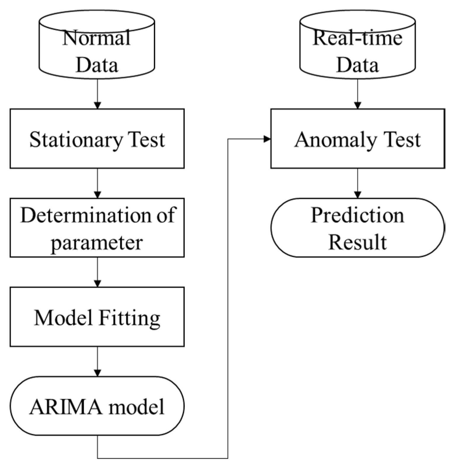
2.1. Statistical Approach

A renowned statistical method, ARIMA (AutoRegressive Integrated Moving Average) has been a cornerstone in time series forecasting for numerous applications. ARIMA’s advantage lies in its ability to capture complex relationships within sequential data, accommodating factors like trend, seasonality, and autocorrelation. By considering the autocorrelations in the data, this method aims to capture and predict underlying patterns in the series. Statistical models offer the advantage of being interpretable, providing insights into the underlying dynamics of the time series. They also offer a structured framework for understanding relationships within the data. However, the choice of model depends on the characteristics of the dataset and the specific forecasting goals. Its adaptability to different domains, robustness in handling noisy data, and provision of interpretable insights make it an indispensable tool for researchers seeking to comprehend and predict intricate temporal behaviors. Its components, AutoRegressive (AR) and Moving Average (MA), along with differencing operations, allow it to model various temporal structures, making it a versatile choice for our dataset.

ARIMA

The ARIMA model was developed by [24]; it combines three elements: AR, MA, and integration (I). It is designed to capture and predict patterns in time series data, which are sequences of data points indexed over time intervals. The model combines AR and MA components with differencing to achieve stationarity. The ARIMA model offers distinct advantages over Bayesian and other statistical models, making it a favorable choice for time series analysis in research articles. Compared to complex Bayesian models that might require substantial computational resources and expertise, ARIMA offers a simpler yet effective approach to modeling and forecasting sequential data [25]. This simplicity translates to ease of implementation and interpretation. ARIMA’s long history in time series analysis provides numerous resources, detailed documentation, and established best practices. This background simplifies model selection, validation, and comparison processes.

The notation for the ARIMA model is ARIMA (p, d, q), where p represents the number of past values used in the autoregression model, d represents the number of difference iterations required to make the time series stationary, and q represents the number of prior residuals used in the moving-average model [26].

The following steps are typically taken to implement an ARIMA model:

• Transform the time series to make it stationary, for example, by differentiation or applying a log transform.
• Assign p, d, and q appropriately. This task can be accomplished by inspecting autocorrelation and partial autocorrelation plots or by applying statistical tests [27].
• Fit the stationary time series to the ARIMA model and make predictions.
• Assess the effectiveness of the ARIMA model by using statistical measures like mean absolute error (MAE), mean square error (MSE), and root mean squared error (RMSE).

The ARIMA model’s complexity and accuracy hinge on the parameters p, d, and q. While there are established procedures to identify suitable values for these parameters [24], for those unfamiliar with these techniques, the process might initially appear daunting. An integral aspect of the ARIMA model is its assumption of stationarity in the series. Thus, non-stationary series need to be transformed accordingly before model implementation.

The values of p, d, and q in an ARIMA model can be calculated in several ways. A common approach is to use time series Autocorrelation Function (ACF) and Partial Autocorrelation Function (PACF) graphs. They can also be determined using automated techniques like auto-ARIMA function and grid search [28,29].

Auto-ARIMA is an algorithmic approach that uses stepwise searches and information criteria (e.g., AIC, BIC) to determine optimal values of p, d, and q. It iteratively explores combinations of orders and selects the combination that has the lowest information criterion score. Auto-ARIMA’s advantage lies in its ability to consider a broad parameter space and adapt to different data characteristics.

Grid Search exhaustively examines a predefined parameter grid to find the combination of p, d, and q that yields the best fit. Grid Search can explore all possible combinations without relying on iterative selection processes. This method could be computationally expensive for large grids.

2.2. Machine Learning Approach

In the context of predicting slope failures, sequential patterns in the data must be identified and understood. ML offers powerful models that are optimized to decipher complex datasets and to extract meaningful information, particularly from time series data [23].

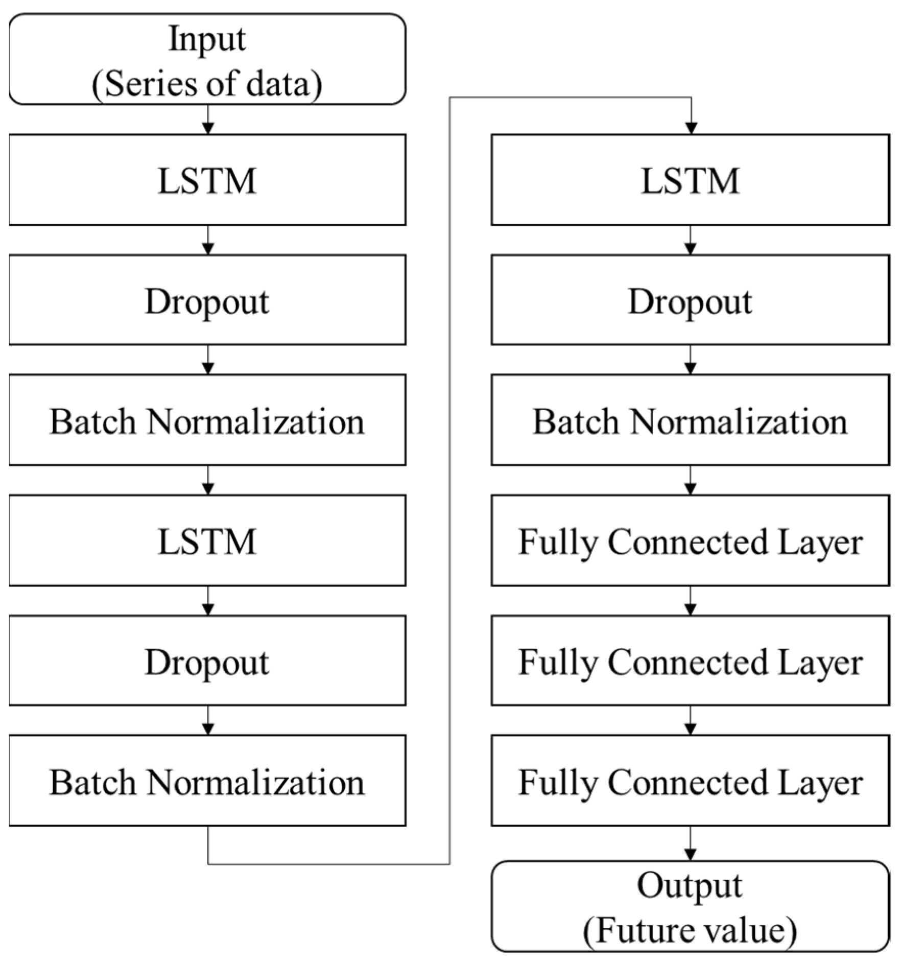
2.2.1. Long Short-Term Memory

Long Short-Term Memory networks (LSTMs) have emerged as an advanced and sophisticated iteration in the continually evolving landscape of neural network architectures, specifically stemming from the lineage of traditional recurrent neural networks (RNNs). The development and adoption of LSTMs were driven primarily by the intrinsic challenges and inefficiencies faced by RNNs, most notably their difficulties in effectively modeling long-term dependencies inherent in sequential data. The hallmark of LSTMs’ architectural prowess lies in their inherent capability to accurately discern and retain intricate patterns even across extended sequences [30]. Such capabilities position LSTMs as an ideal candidate for handling time series data, as underscored by their instrumental role in high-stakes applications, including the prediction of slope failures.

LSTMs, a variant of Recurrent Neural Networks (RNNs), were developed to address the limitations of traditional RNNs, including challenges like the ‘vanishing gradient’ problem [31], which can hinder the network’s ability to recognize long-term dependencies in sequential data [32]. LSTMs introduce an innovative architectural solution: a collection of specialized gating structures. These gates, encapsulating the input, forget, and output gate mechanisms, are meticulously designed to oversee, modulate, and regulate the flow and transformation of information through the network [32]. These gates have the capacity to judiciously determine the fate of incoming data—whether to retain, modify, or discard it. This granular, data-centric decision-making ability empowers LSTMs to outperform RNNs in managing and harnessing information across vast temporal spans. These gates dynamically adapt to the evolving context, making informed choices on which sequence fragments are integral for retention and which can be disregarded. This contextual, adaptive memory management, quintessential to LSTMs, ensures not merely an efficient absorption of past sequence intricacies but also the adept utilization of this accumulated knowledge to derive precise future predictions. LSTMs, due to their capability to capture long-term dependencies in sequential data, have seen applications not just in general time series forecasting but also in specific domains such as earthquake engineering. For instance, Ref. [33] utilized LSTMs, alongside WaveNet and 2D CNN, for nonlinear time history prediction of seismic responses. Similarly, Ref. [34] employed deep learning methods, including LSTMs, to estimate seismic demand models of building inventories based on nonlinear static analyses. These studies underscore the versatility and potential of LSTMs in addressing intricate geotechnical problems.

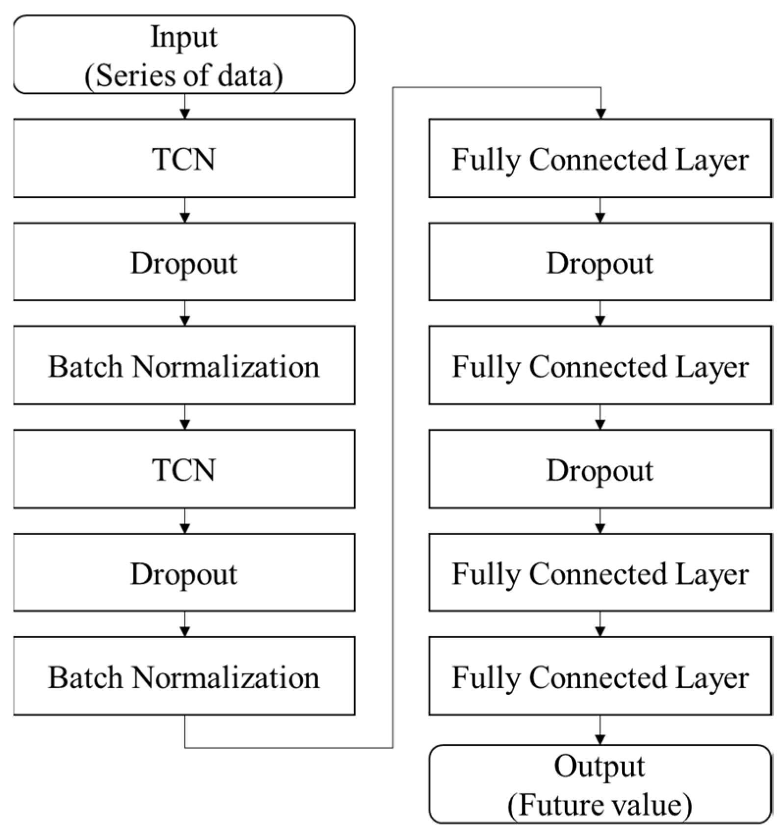
2.2.2. Temporal Convolutional Network (TCN)

Temporal Convolutional Networks (TCNs) have emerged as a significant advancement in neural network architectures, specifically tailored for processing sequential and time series data. Unlike traditional convolutional networks, which excel in spatial feature extraction as observed in image processing, TCNs are designed to harness the temporal dynamics intrinsic to sequential data [35]. This makes them particularly relevant for applications that require a deep understanding of time dependencies. Conventional convolutional networks, while proficient at spatial feature extraction, struggle when the data’s temporal relationships are paramount. In response to this challenge, TCNs introduce several architectural innovations. They employ dilated convolutions to expand the network’s receptive field without increasing the number of parameters or computational complexity, thereby capturing long-range temporal dependencies efficiently [36]. Additionally, TCNs use causal convolutions, ensuring predictions at any given time step are influenced solely by past and current data, upholding the integrity of temporal sequences [37].

Moreover, the TCN architecture naturally integrates residual connections; this structure promotes efficient gradient flow and addresses challenges associated with training deep networks [38]. Because of these residual connections, the network can learn residual mappings, addressing the vanishing gradient problem and improving information transfer across layers. One of the notable advantages of TCNs is their flexibility [39]. They can be adeptly scaled in terms of depth and receptive field size, accommodating datasets of diverse complexities. Given their ability to capture both short-term and long-term dependencies and being free from pitfalls like the vanishing gradient problem inherent to recurrent architectures like RNNs, TCNs are positioned as promising candidates for rigorous sequential data analysis and prediction.

TCNs can process multiple sequence segments concurrently, distinguishing them from RNNs, which are inherently sequential and computationally intensive. This parallel processing capability, coupled with the model’s scalability, ensures rapid training and effective deployment on GPUs and distributed systems. Furthermore, models like TCNs can be trained using conventional backpropagation algorithms such as stochastic gradient descent (SGD) or Adam, with the choice of loss function depending on the specific task, such as mean square error for regression or cross-entropy loss for classification (Bai et al., 2018).

2.3. Performance Assessment

In the realm of predicting slope failures, where the timeliness and consistency of warnings can be critical, traditional performance metrics may fall short. Given the unique challenges of this domain, including ambiguous labeling, it becomes imperative to craft a custom evaluation metric that captures the nuance of effective early warnings. Given a set S of slope failures and associated warnings Wi for the i-th slope failure, and a set F of false alarms, we introduce a composite metric designed to balance timely prediction, penalization of false alarms, and the reward for consistent warning sequences.

Key Definitions:

• T: Ideal warning window preceding a slope failure.
• Δ: Time span to evaluate consecutive false alarms.
• $t_i$: Time of the i-th slope failure.
• l (condition): Indicator function; 1 if the condition is true, 0 otherwise.

The performance score P is thus defined as:

$$\begin{gathered} \mathrm{P}={\sum }_{i=1}^{\left|S\right|}(\alpha \times l\left(\mathrm{a}\mathrm{n}\mathrm{y} \mathrm{w}\mathrm{a}\mathrm{r}\mathrm{n}\mathrm{i}\mathrm{n}\mathrm{g} \mathrm{i}\mathrm{n} \left|t_i-T, t_i\right|\right))+\beta \times \mathrm{n}\mathrm{u}\mathrm{m}\mathrm{b}\mathrm{e}\mathrm{r} \mathrm{o}\mathrm{f} \mathrm{c}\mathrm{o}\mathrm{n}\mathrm{s}\mathrm{e}\mathrm{c}\mathrm{u}\mathrm{t}\mathrm{i}\mathrm{v}\mathrm{e} \mathrm{w}\mathrm{a}\mathrm{r}\mathrm{n}\mathrm{i}\mathrm{n}\mathrm{g}-\gamma \times \\ l\left(\mathrm{n}\mathrm{o} \mathrm{w}\mathrm{a}\mathrm{r}\mathrm{n}\mathrm{i}\mathrm{n}\mathrm{g} \mathrm{i}\mathrm{n} \left|t_i-T, t_i\right|\right)-{\sum }_{j=1}^{\left|F\right|}A\times (1+l(\mathrm{n}\mathrm{e}\mathrm{x}\mathrm{t} \mathrm{f}\mathrm{a}\mathrm{l}\mathrm{s}\mathrm{e} \mathrm{a}\mathrm{l}\mathrm{a}\mathrm{r}\mathrm{m} \mathrm{w}\mathrm{i}\mathrm{t}\mathrm{h}\mathrm{i}\mathrm{n} \mathsf{\Delta })) \end{gathered}$$

(1)

where, $\alpha , \beta , \gamma , \mathrm{a}\mathrm{n}\mathrm{d} A$ are weighing coefficients.

Slope failure predictions are most valuable within a specific time window. A warning that is too early might lead to unnecessary preventive actions, whereas a warning that is too late is ineffective. Thus, warnings within a designated window, T, are rewarded. Intermittent or sporadic warnings might lead to distrust or confusion. Consecutive warnings within the ideal window provide consistent indicators, and thereby increase trust and allow for timely interventions. A system that does not warn within the ideal window might lead to unmitigated risks. Such misses are heavily penalized. While timely warnings are critical, false alarms can erode trust in the system. Therefore, false alarms are penalized, with increasing penalties for consecutive false alarms in a short time span, Δ. The proposed evaluation metric provides a balanced approach to assess the effectiveness of early warning systems for slope failures. In short, the first term rewards with $\alpha$ points if there is any warning in the ideal window before the slope failure. The second term gives additional rewards for consecutive warnings in the window leading to the slope failure. The third term penalizes by $\gamma$ points if no warning is given in the window before the slope failure. The last term penalizes by A points for a false alarm, and double that if the next false alarm is within Δ time span. It uniquely combines principles from signal detection theory, time series forecasting, and reinforcement learning, tailoring them for the domain-specific challenges of predicting slope failures We adjusted performance ranges from zero (just detect slope failure when it occurs) to one (perfect prediction) as below.

$$P_{adjusted}=\frac{P-P_{min} }{P_{max}-P_{min}}$$

(2)

where $P_{max}$ is the maximum possible score and $P_{min}$ is the minimum possible score. This transformation can convert $P_{adjusted}$ range between zero and one.

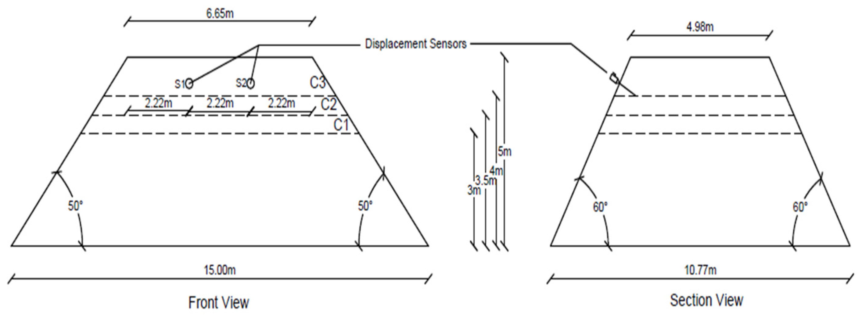
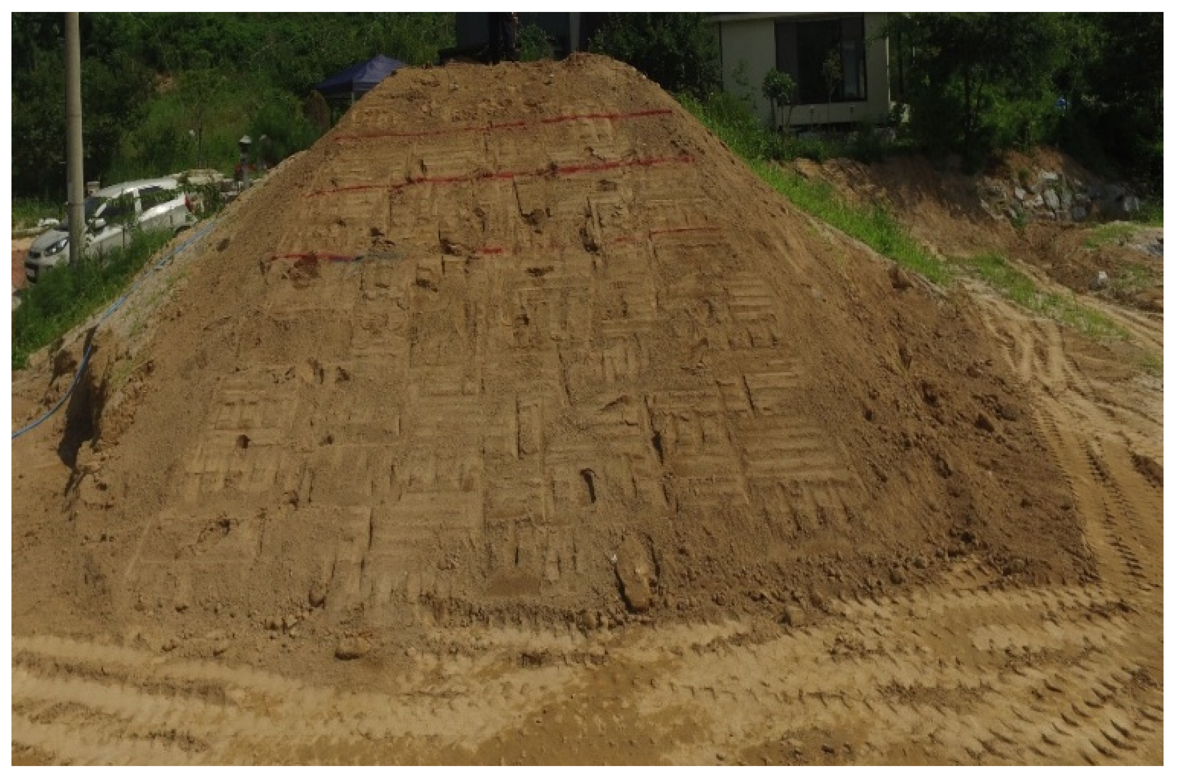
2.4. Design of Field Model Slope

A slope was prepared by the stepwise filling method and a field experiment was conducted, cutting the slope stepwise through each cut section. The height of the slopes was determined using numerical analysis and the model slope during the field experiment was designed as per the result of the numerical analysis. The slope model was prepared with a crest height of 5 m and crest length of 6.65 m. The slope angle was maintained to be 60° as illustrated in Figure 1. Two displacement sensors were used, S1 and S2, each of lengths of 1000 mm and 800 mm, respectively. The response of the sensors was tested before the field experiment was carried out. These sensors were considered in cantilever condition, with one fixed end and another free end during the execution of this field experiment.

Mountain ranges in South Korea are mostly formed by tectonic activities and erosional deposits [40,41]. While most slopes are made of impermeable rocks, some slopes have a shallow top layer of permeable soil that is less than 1 m deep. In Korea, rocky slopes make up more than 78% of cut slopes and about 79% of slopes that are prone to landslides [42]. Also, the predominant slopes consist of weathered rocks. Most natural slopes of South Korea are structurally weak and prone to landslides, especially during rainy seasons.

Weathered granite soil, which is widely distributed in South Korea, was used in this field test. These soils are mostly used as base materials and filling materials in construction works. Genesis rocks are weathered by various processes, and they develop several voids and large deformation occurs when internal or external forces are encountered. The soil used in this study is SW soil as per the Unified Soil Classification System (USCS), with the physical properties as per

Table 1. Physical properties of soil used for model preparation.

Physical Properties	Values
Density of soil	17.9 kN/m3
Sand	57.5%
Clay	1.5%
Silt	10%
D50	0.85 mm
Maximum dry density	19.3 kN/m3
Optimum water content	13%

. A field density test was conducted to obtain the unsaturated state of this soil material and compaction tests were adjusted and applied in the field experiment. The model slope was prepared using a backhoe, but no compaction was performed by the bucket of the backhoe. Only the self-weight of the soil was applied to construct the model slope to resemble the natural decomposition conditions.

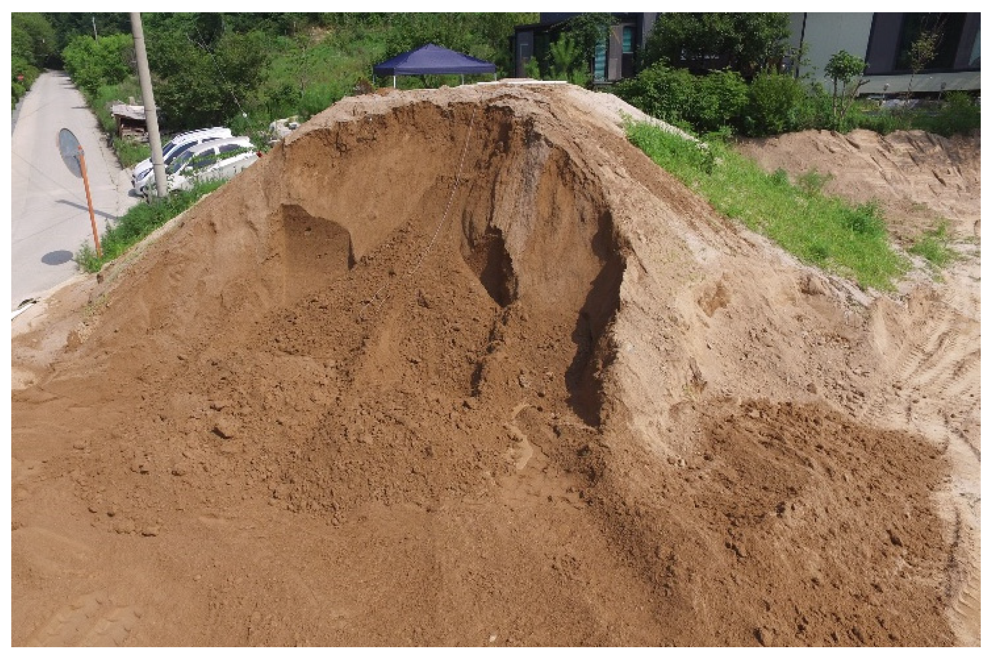
2.5. Installation of Subsurface Displacement Sensors and Simulation of Slope Failure

Using the penetration screws fastened to the lower part of the sensor, the displacement sensors were mounted perpendicular to the slope surface. The sensors were installed at a horizontal spacing of 2.22 m. Stepwise cutting was started from the slope’s toe and the slope failure behavior was observed. From the initial excavation work (C1) to the third (C3), mentioned by red lines in Figure 2 the excavation was executed in three distinct phases, ensuring that the excavated surface remained vertical.

The duration for each excavation phase, encompassing the interim period post-excavation, spanned 20 min. Continuous assessments were conducted to capture potential discrepancies between consecutive excavation phases. Displacement data were amassed at intervals of one second.

Figure 2 shows the field model slope, while Figure 3 shows the cutting process of the field slope and Figure 4 shows the field slope after failure.

3. Experiment

In this section, the data collected during this phase serve as the basis for the subsequent development of an ML model that has the goal of predicting slope failure.

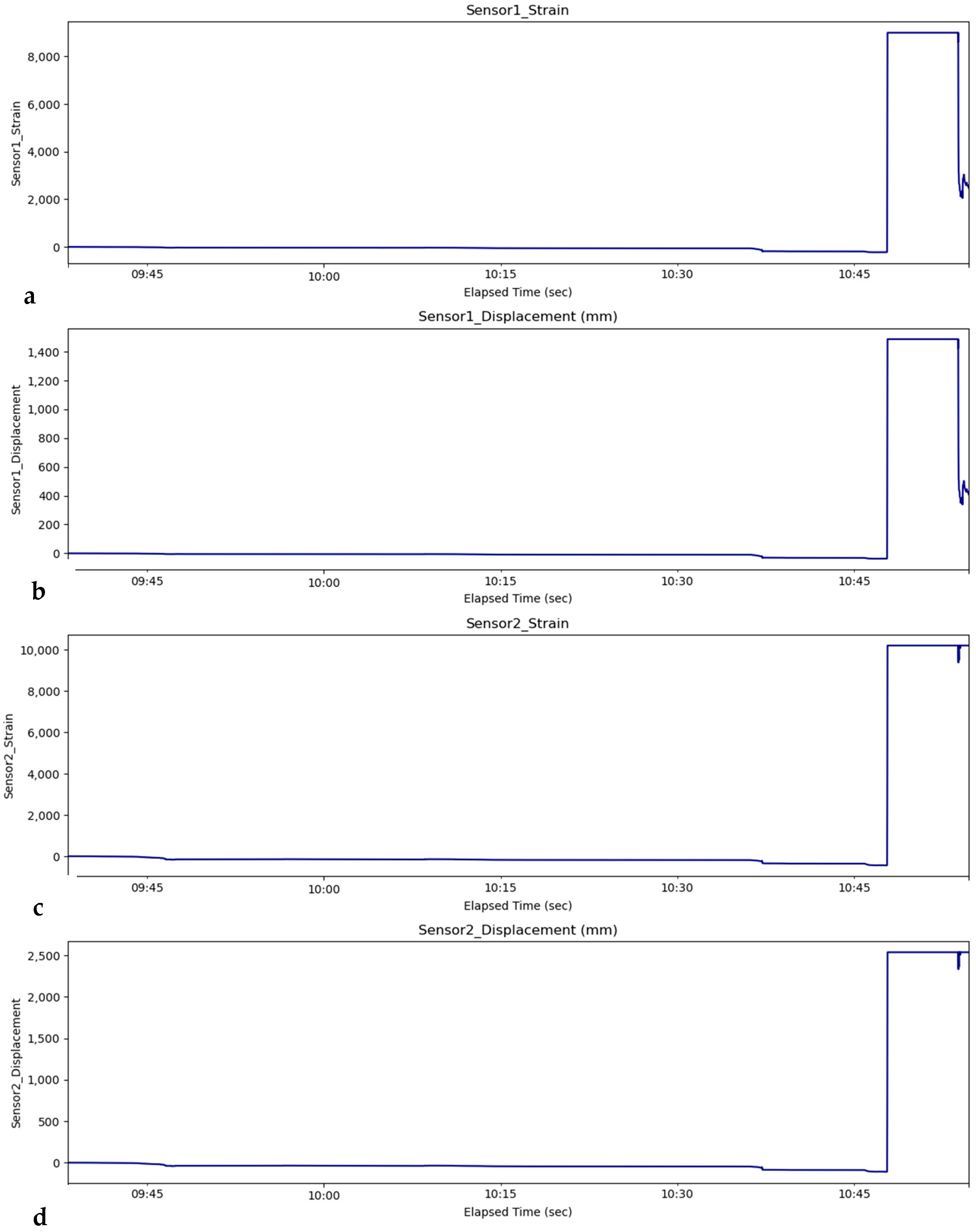
3.1. Data Description

The slope was initially in a stable condition; for the experiment, it was cut vertically at three times: C1 at 9:58, C2 at 10:18, and C3 at 10:38 a.m. Following these interventions, the slope experienced a rapid failure at 10:45 a.m. The primary instrument used for data collection during this period was the strain gauge, which possesses the capability to measure displacement. The data collection spanned from 9:38 to 10:54, resulting in a comprehensive set of 4586 data points. The gathered data are visually represented across four distinct plots. Figure 5a portrays the time on the x-axis against the strain from sensor 1 on the y-axis. Figure 5b uses the same temporal x-axis but has a y-axis of displacement (in millimeters) from Sensor 1. The narrative continues with Figure 5c, which displays time on the x-axis and strain readings from Sensor 2 on the y-axis. Concluding the series, Figure 5d offers a visual of the time against the displacement, also measured in millimeters.

3.2. Prediction Model Development

This section describes the techniques that were used to formulate the statistical and ML prediction models for slope failure. The methodologies are classified into two main categories: statistical and machine learning approaches.

3.2.1. Statistical Approach

The ARIMA model was used in this study to forecast the future value and determine the anomaly. The work used a thorough method for series-data forecasting and anomaly identification by using Python’s ARIMA model in the Google Collaboratory environment. The ARIMA process (Figure 6) was conducted in six steps divided into two phases, one for calibration using data from a stable slope (“Normal data”) and one using data from an unstable slope (“Real-time data”).

In our pursuit to develop a robust slope failure prediction model, we employed ARIMA. The process commenced with collecting and pre-processing normal data, which formed the foundation for the training and validation of the slope failure prediction model. Recognizing the importance of stationarity in ARIMA modeling, stationarity tests were conducted before the determination of the parameters. Augmented Dickey–Fuller (ADF) tests were used for the stationary test. In instances where the data exhibited non-stationarity, transformation measures, notably differencing, were applied to achieve a stationary state. After confirming the stationarity of the dataset, the next critical step was parameter determination. The order of differencing, represented as ‘d’, was deduced based on the extent required to attain a stationary time series. For the identification of the optimal number of Moving Average (MA) terms (q), the Autocorrelation Function (ACF) plot proved instrumental. Similarly, the Partial Autocorrelation Function (PACF) plot was employed to ascertain the optimal number of Autoregressive (AR) terms (p). Once the parameters (p, d, q) were systematically determined, we fit the ARIMA model to the normal dataset. This phase involved validating the model on a distinct data subset, frequently adopting a rolling forecast approach for an in-depth performance assessment. The true efficacy of the model was evaluated during the slope failure prediction phase. A test dataset was introduced, encompassing values from slopes of unknown stability. Each data point from this new set was forecast using the ARIMA model, and the difference between the observed and predicted values was diligently computed. To interpret these differences in the context of slope stability, we established a threshold grounded in our understanding of the normal data. This threshold encapsulated the maximum allowable difference under normal conditions. Any deviation surpassing this defined threshold signaled an unstable slope condition. In contrast, minor deviations within the threshold bounds indicated a stable slope state.

3.2.2. Machine Learning Approach

Integrating machine learning techniques has emerged as a pivotal advancement in slope failure prediction, enhancing our predictive capabilities. Our methodology emphasizes forecasting future values based on data derived from stable slope conditions. Central to this strategy is the assertion that when crossing a defined threshold, notable divergences between real-time observations and their corresponding predicted values can signify impending slope disruptions. We can effectively discern signs of slope instability by evaluating the difference between predicted future values and actual recorded data (Figure 7). If the variance between these values is within the prescribed threshold, it confirms the slope’s stability. In contrast, deviations beyond this benchmark serve as critical early warning signals, pointing to potential imminent slope failures. Our methodology, while building upon established ML algorithms like LSTM and TCN, offers a tailored approach to address the specific challenges inherent in predicting slope failures.

LSTM-Based Model

The model designed for slope failure prediction is an advanced deep learning architecture that capitalizes on the capabilities of Long Short-Term Memory (LSTM) networks, renowned for adeptly handling time series data (Figure 8). The architecture initiates with an input shaped by the “window size” spanning over four features, representing the number of past time steps that are considered when making predictions. This feeds into the first LSTM layer, which comprises 100 units and is set to return sequences. This means it provides an output of the same length as the input to pass on to the subsequent LSTM layer. To augment the model’s generalization and curtail potential overfitting, a dropout rate of 20% is infused, followed by batch normalization to stabilize the learning process. A similar design pattern persists into the second LSTM layer, which consists of 100 units and returns sequences. Again, a 20% dropout rate is implemented, accompanied by batch normalization. Diverging slightly, the third LSTM layer also consists of 100 units, but does not return sequences; instead, it offers a consolidated output for the following layers. Consistent with the earlier LSTM layers, this layer incorporates a 20% dropout and batch normalization.

After the LSTM layers, the architecture introduces two dense or fully connected layers to further refine the features. The initial dense layer activates 50 neurons using the Rectified Linear Unit (ReLU) activation function. This infuses the model with the necessary non-linearity, and thereby empowers it to discern complex patterns. A successive dense layer is equipped with 25 neurons, which leverage the ReLU activation.

The final output layer Is a dense”conf’guration with four neurons. Given the regression-oriented nature of the slope failure prediction task, this layer abstains from using an explicit activation function. The Adam optimizer, a widely adopted optimization algorithm befitting deep learning tasks, is selected during the model’s compilation phase. The Mean Squared Error (MSE) is the chosen loss function, ideal for regression endeavors, as it computes the average squared difference between the anticipated and actual values.

This model has been meticulously tailored to discern the temporal intricacies and nuanced patterns inherent in slope data, paving the way for a robust predictive mechanism for potential slope failures.

TCN-Based Model

In the developed model for slope failure prediction, we leverage the Temporal Convolutional Network (TCN) architecture, renowned for its proficiency in managing sequential data, akin to Recurrent Neural Networks, but often with superior training efficiency and parallelization capabilities. The model commences with an initial TCN layer configured with an input shape corresponding to the window size and feature dimensions. This layer boasts 150 filters, a kernel size of three, and dilation rates spanning [one, two, four, eight], expanding the receptive field and enabling the model to recognize patterns over diverse time scales. To prevent potential overfitting due to the increased complexity, a 30% dropout rate follows this layer. A batch normalization is also incorporated, optimizing the internal layer dynamics and accelerating the training process. After the initial TCN layer, the model integrates another TCN layer with 100 filters, a kernel size of two, and dilation rates of [one, two, four]. The purpose of this subsequent layer is to extract further and refine the features derived from the first TCN layer. The output from the final TCN layer is then propagated through dense layers. Beginning with a 100-neuron layer, it sequentially funnels through layers with 50 and 25 neurons. These dense layers play a pivotal role in decoding the features gleaned from the temporal convolutions and translating them into representations conducive to our predictive task. Intermittent dropout layers, with a rate of 20%, are situated between these dense layers to bestow further regularization, ensuring that the model remains robust and resistant to overfitting. Concluding the architecture, the model incorporates an output layer with four neurons, mirroring the number of prediction targets. The model is compiled with the Adam optimizer and a mean squared error loss, attesting to its regression-oriented nature. With its compounded TCN layers and dense interpretative layers, this architecture is poised to capture the intricate temporal patterns and nuanced relationships in the data, facilitating a robust predictive mechanism for slope failure detection. The architectural layout of a TCN model is detailed in Figure 9.

4. Result

This section presents the findings obtained from deploying the developed prediction models. As the primary focus of this research lies in comprehending the efficacy and precision of the models in predicting slope failures, it is crucial to delineate the results in an organized and detailed manner. We begin with a comprehensive analysis of the anomaly detection outcomes. Following this, the models’ performance metrics are discussed, showcasing their respective strengths and areas of improvement. This section also presents a comparative analysis, comparing the results obtained from the statistical and machine learning approaches.

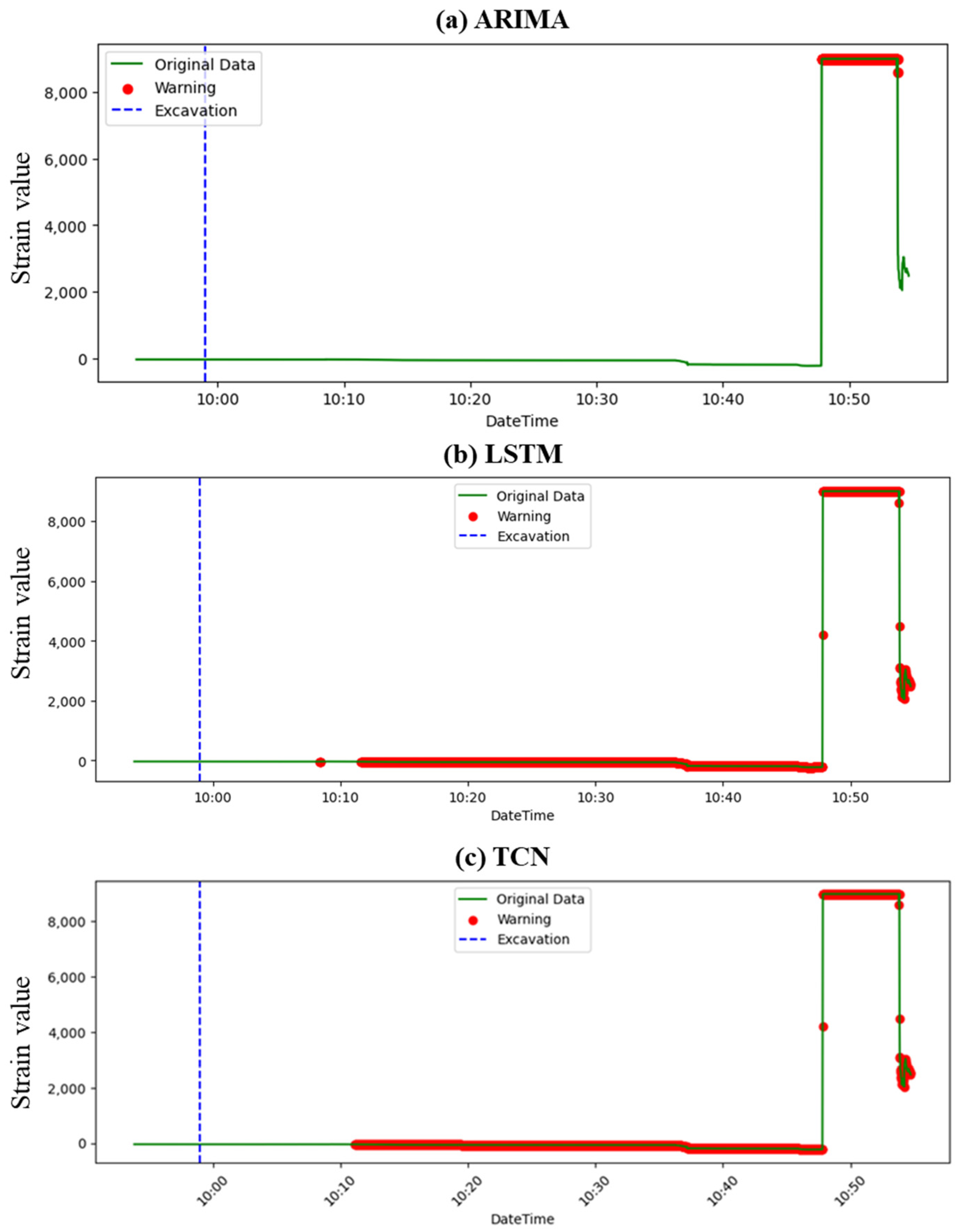
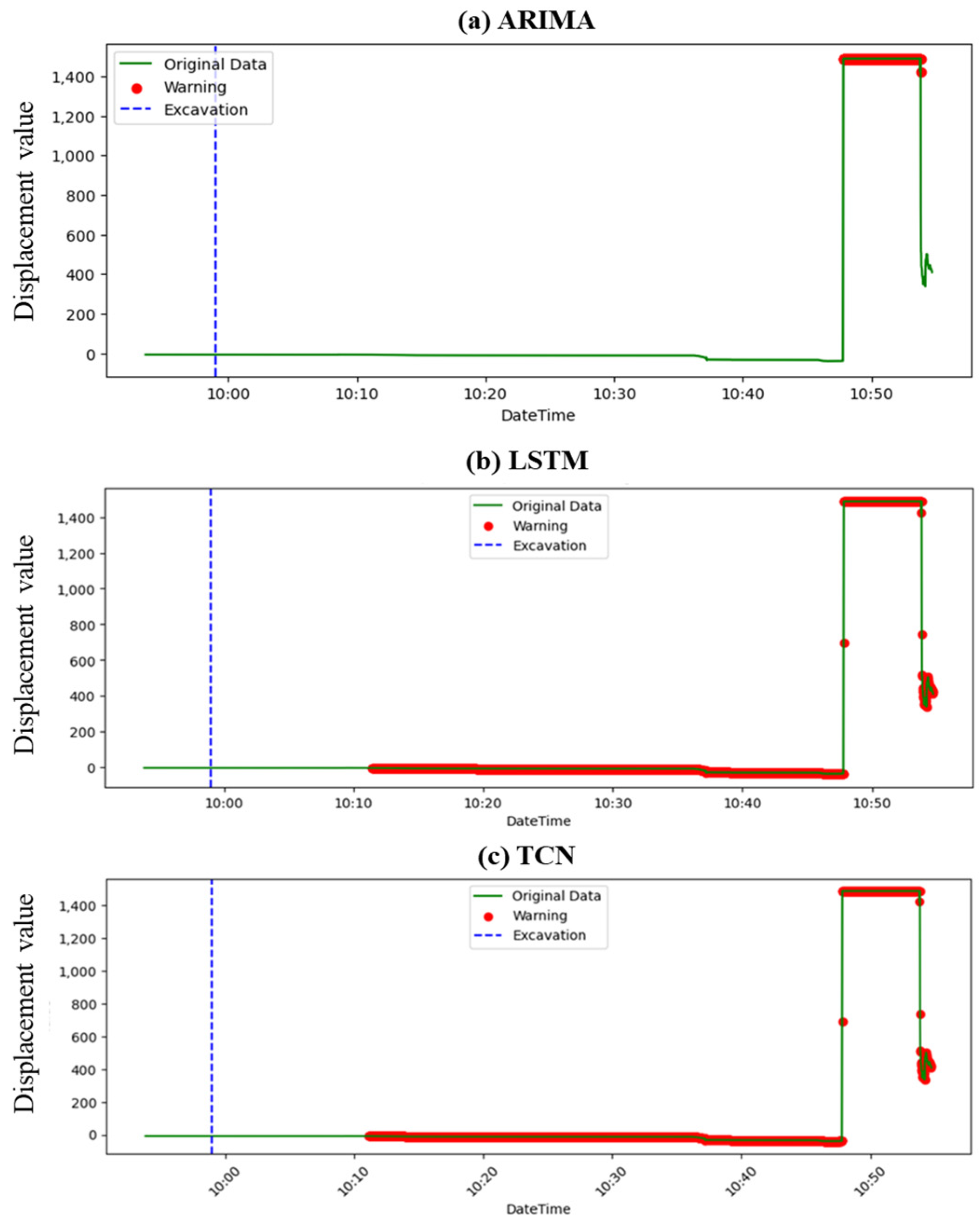
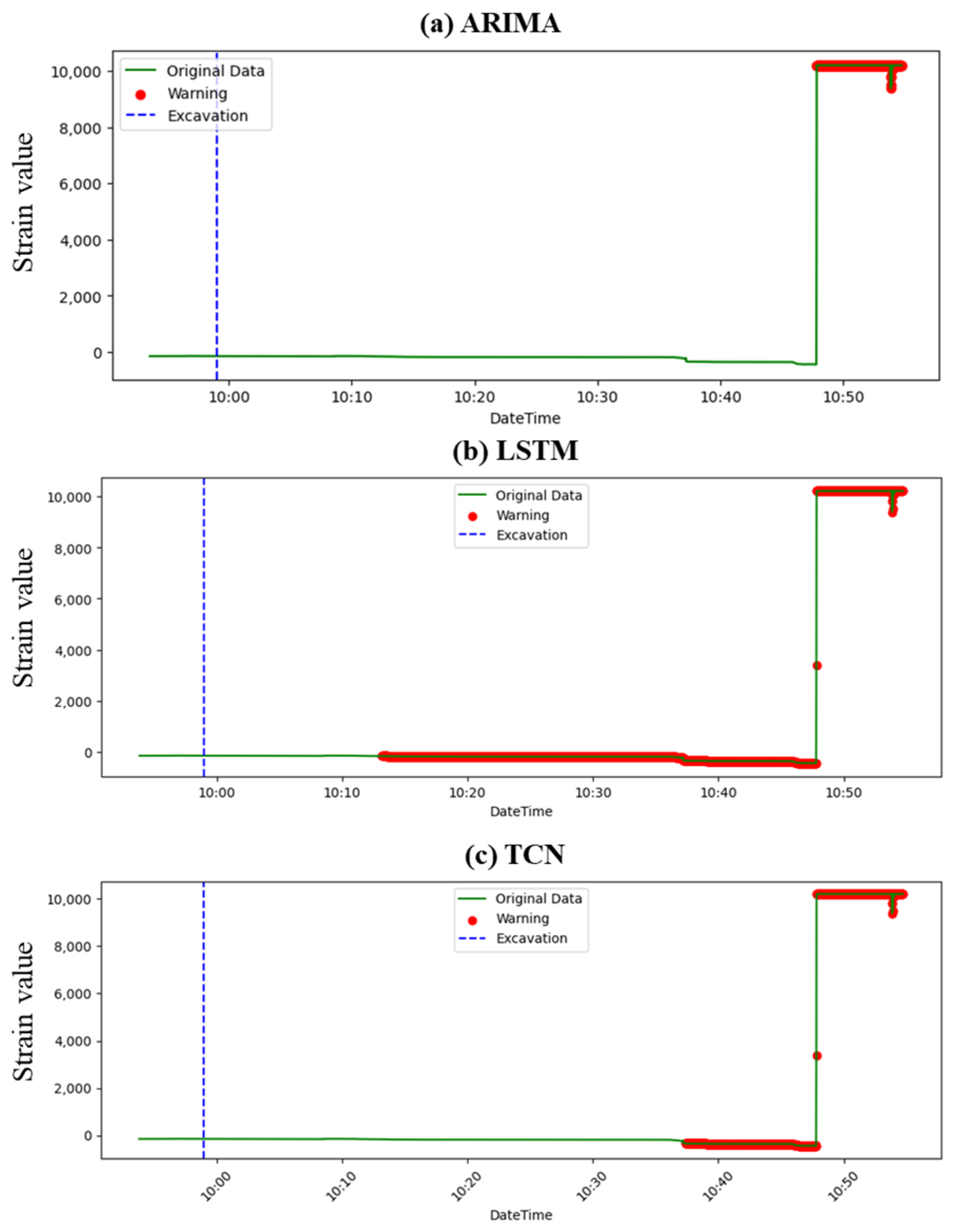
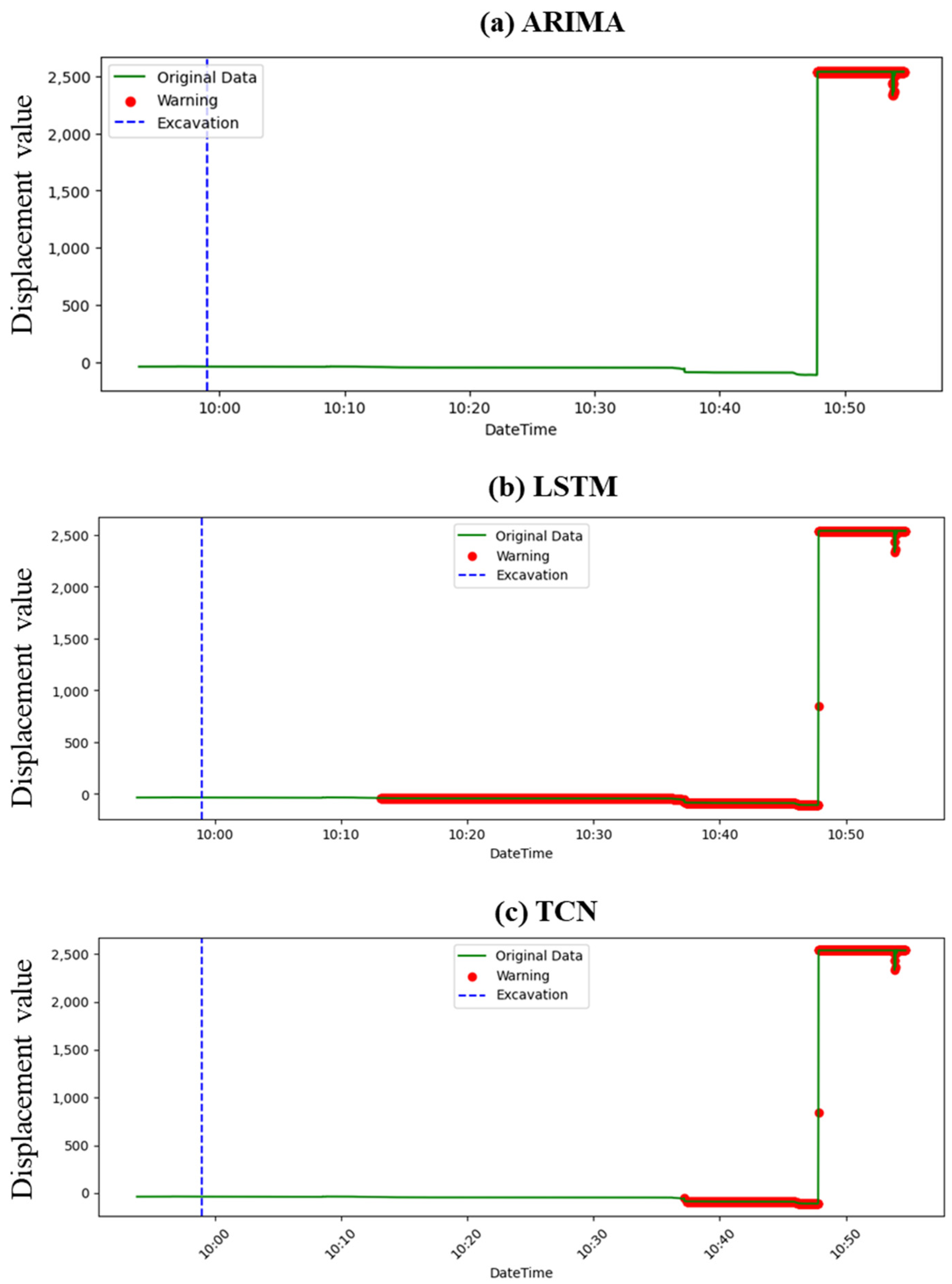
4.1. Prediction Result

The slope failure prediction utilized four types of data: strain from Sensor 1 (Figure 10), displacement from Sensor 1 (Figure 11), strain from Sensor 2 (Figure 12), and displacement from Sensor 2 (Figure 13). When using strain data from Sensor 1, the ARIMA model predicted slope failure immediately after the actual failure occurred at 10:47:47 (Figure 10a). In contrast, the LSTM model started to predict slope failure from 10:07:39 to 10:08:32 (Figure 10b), but it also indicates stable status in the overlapping period from 10:08:22 to 10:11:25, which could lead to ambiguity in interpretation. Subsequently, it continued to issue warnings until the end of the dataset. The TCN model raised a warning at 10:11:46, approximately 36 min before the actual slope failure (Figure 10c). Although this warning was slightly delayed compared to the LSTM model’s prediction, the TCN model consistently maintained its warning state, so confusion about the interpretation is not possible.

When using the displacement from Sensor 1, the prediction results were slightly different from those obtained using the strain data. The ARIMA model once again did not furnish a proactive warning (Figure 11a). However, both the LSTM (Figure 11b) and TCN (Figure 11c) models issued continuous alerts before the actual slope failure. Interestingly, both LSTM and TCN started issuing warnings at 10:11:46; this synchroneity may be a result of the characteristics of the dataset, or both models may have identified the same pattern as critical for predictions.

The predictive outcomes varied once again when employing the third dataset, specifically the strain measurements from Sensor 2. As depicted in Figure 12, the ARIMA model could not provide a preemptive alert. In contrast, the LSTM model gave an early warning at 10:13:26. This initiation of warning was slightly delayed by approximately 100 s compared to its performance with the previous dataset. Meanwhile, the TCN model’s alert was significantly belated, initiating roughly 20 min after the LSTM’s warning at 10:36:27. The earlier warning by the LSTM in this instance could be attributed to its ability to better capture temporal dependencies within the strain data from Sensor 2.

When the displacement data from Sensor 2 were used, the predictive outcomes were nearly identical to those obtained using the strain data of Sensor 2. The ARIMA model could not render an advanced alert (Figure 13a). The LSTM model issued a warning at 10:13:27 (Figure 13b), which was 23 min earlier than the TCN’s alert at 10:36:27 (Figure 13c). This time difference is further evidence that the LSTM is better than the TCN at detecting intricate temporal patterns and dependencies in the displacement data from Sensor 2.

4.2. Performance Assessment

We used the performance metric suggested in Section 2 and Section 3. In analyzing the results, it becomes evident that the LSTM model consistently demonstrates a superior capability to detect early signs of slope failures across all sensor data types, as shown in

Table 2. Prediction performance P_adjusted (Equations (1) and (2)) of ARIMA, LSTM, and TCN in slope failure prediction.

	Statistical	Machine Learning
	ARIMA	LSTM	TCN
Sensor1_strain	0	0.81	0.78
Sensor1_dispacement	0.12	0.79	0.78
Sensor2_strain	0	0.76	0.69
Sensor2_dispacement	0.14	0.78	0.69

. Its scores are higher in comparison to both the TCN and the ARIMA models. This suggests that the LSTM model, a type of recurrent neural network, is adept at recognizing patterns over extended time intervals and is particularly effective for time series forecasting in the context of this study. While the TCN also showcases proficiency in handling time series data, its performance slightly trails that of the LSTM. The TCN employs causal convolutions to ensure that predictions at any given time rely solely on past information. This capability allows it to capture patterns over time, albeit not as effectively as the LSTM in this dataset. On the other hand, ARIMA, a linear time series forecasting model, appears to have limitations in capturing complex patterns inherent in the dataset. This model, which operates based on autoregression, differencing, and moving averages, might be struggling to identify more intricate, non-linear patterns. This is further reflected in its diminished scores for both strain and displacement data from the sensors. Moreover, the almost negligible performance of the statistical methods indicates potential insensitivity to the specific patterns of slope failures present in this dataset. The low scores, especially zeros in cases involving strain data, might suggest that these methods either require a richer dataset or lack the sensitivity necessary for this specific application. It is also worth noting the differences in scores between strain and displacement data. Generally, regardless of the model employed, strain data yield higher scores even though the displacement is derived from strain.

5. Conclusions

This study aimed to evaluate the efficacy of various models in predicting slope failures using data obtained from two sensors, each measuring strain and displacement. Recognizing a gap in the existing literature, we addressed the absence of a dedicated performance metric for slope failure prediction and proposed a novel one to better assess the prediction accuracy of the models. Also, four distinct datasets were analyzed employing three predictive models: ARIMA, LSTM, and TCN. Here are the salient conclusions drawn:

• Comparative efficacy: Across the datasets, the ARIMA model consistently showed limitations in providing timely warnings prior to slope failures. In contrast, LSTM and TCN demonstrated more promising capabilities, with LSTM consistently outperforming the other models regarding the timeliness of its warnings.
• Data source insights: While the nature of data (strain or displacement) impacted prediction capabilities somewhat, the source of data (Sensor 1 or Sensor 2) seemed to have a more pronounced effect. Predictions were remarkably similar when models used strain and displacement data from the same sensor. This can be attributed to the fact that displacement values are derived from strain measurements, leading to inherent correlations between the two types of data.
• LSTM outperforms others: LSTM’s recurrent nature, enabling it to retain memory from prior data in sequences, likely contributed to its enhanced performance. Especially for events like slope failures where historical data play a crucial role in prediction, LSTM’s ability to capture long-term dependencies proved invaluable.
• Timeliness vs. consistency: While LSTM provided earlier warnings, TCN’s consistency in providing continuous alerts, even if slightly delayed, highlighted the potential trade-off between early prediction and sustained warning periods. This distinction is crucial for practical applications where consistent warnings might be preferred over sporadic early alerts.
• Implications for field applications: This study’s findings suggest that for real-world applications, employing LSTM models can significantly enhance the lead time for slope failure warnings, granting authorities a better window for preventive measures. However, the choice between LSTM and TCN would hinge on specific on-ground requirements—whether early warning or continuous alert consistency is more critical.

In conclusion, although both machine learning-based models offered significant insights, LSTM was identified as the most effective for slope failure prediction in this investigation. Future research could focus on fine-tuning its parameters or consider hybrid approaches that capitalize on the strengths of multiple models. Incorporating other external factors and data sources is also advisable to further refine prediction accuracy.

References

- Alfieri, L.; Salamon, P.; Pappenberger, F.; Wetterhall, F.; Thielen, J. Operational early warning systems for water-related hazards in Europe. Environ. Sci. Policy 2012, 21, 35–49. [Google Scholar] [CrossRef]
- Barredo, J.I. Normalised flood losses in Europe: 1970–2006. Nat. Hazards Earth Syst. Sci. 2009, 9, 97–104. [Google Scholar] [CrossRef]
- European Environment Agency. Mapping the impacts of natural hazards and technological accidents in Europe An overview of the last decade. In Technical Report No 132010; European Environment Agency: Copenhagen, Denmark, 2010; Issue 13. [Google Scholar] [CrossRef]
- Piciullo, L.; Calvello, M.; Cepeda, J.M. Territorial early warning systems for rainfall-induced landslides. Earth-Sci. Rev. 2018, 179, 228–247. [Google Scholar] [CrossRef]
- Kim, Y.S. Development of Slope Failure Forecasting and Warning System; Research Institute Report: Seoul, Republic of Korea, 2015. (In Korean) [Google Scholar]
- Froude, M.J.; Petley, D.N. Global fatal landslide occurrence from 2004 to 2016. Nat. Hazards Earth Syst. Sci. 2018, 18, 2161–2181. [Google Scholar] [CrossRef]
- Shanmugam, G.; Wang, Y. The landslide problem. J. Palaeogeogr. 2015, 4, 109–166. [Google Scholar] [CrossRef]
- Nepal, N.; Chen, J.; Chen, H.; Wang, X.; Pangali Sharma, T.P. Assessment of landslide susceptibility along the Araniko Highway in Poiqu/Bhote Koshi/Sun Koshi Watershed, Nepal Himalaya. Prog. Disaster Sci. 2019, 3, 100037. [Google Scholar] [CrossRef]
- Sassa, K.; Wang, G.; Fukuoka, H.; Wang, F.; Ochiai, T.; Sugiyama, M.; Sekiguchi, T. Landslide risk evaluation and hazard zoning for rapid and long-travel landslides in urban development areas. Landslides 2004, 1, 221–235. [Google Scholar] [CrossRef]
- Maxwell, A.E.; Sharma, M.; Donaldson, K.A. Explainable boosting machines for slope failure spatial predictive modeling. Remote Sens. 2021, 13, 4991. [Google Scholar] [CrossRef]
- Zaker Esteghamati, M.; Kottke, A.R.; Rodriguez-Marek, A. A Data-Driven Approach to Evaluate Site Amplification of Ground-Motion Models Using Vector Proxies Derived from Horizontal-to-Vertical Spectral Ratios. Bull. Seismol. Soc. Am. 2022, 112, 3001–3015. [Google Scholar] [CrossRef]
- Bishop, A.W. The use of the Slip Circle in the Stability Analysis of Slopes. Géotechnique 1955, 5, 7–17. [Google Scholar] [CrossRef]
- Janbu, N. Application of composite slip surfaces for stability analysis. Eur. Conferr. Stab. Earth Slopes 1954, 3, 43–49. Available online: https://api.semanticscholar.org/CorpusID:131229483 (accessed on 12 June 2023).
- Morgenstern, N.R.; Price, V.E. The Analysis of the Stability of General Slip Surfaces. Géotechnique 1965, 15, 79–93. [Google Scholar] [CrossRef]
- Spencer, E. A Method of analysis of the Stability of Embankments Assuming Parallel Inter-Slice Forces. Géotechnique 1967, 17, 11–26. [Google Scholar] [CrossRef]
- Duncan, J.M. State of the Art: Limit Equilibrium and Finite-Element Analysis of Slopes. J. Geotech. Eng. 1996, 122, 577–596. [Google Scholar] [CrossRef]
- Chakraborty, A.; Goswami, D. Two Dimensional (2D) Slope-Stability Analysis—A review. Int. J. Res. Appl. Sci. Eng. Technol. 2018, 6, 2108–2112. [Google Scholar]
- Zienkiewicz, O.C.; Taylor, R.L. The Finite Element Method Volume 1: The Basis. Methods 2000, 1, 708. [Google Scholar]
- He, L.; Gomes, A.T.; Broggi, M.; Beer, M. Failure analysis of soil slopes with advanced Bayesian networks. Period. Polytech. Civ. Eng. 2019, 63, 763–774. [Google Scholar] [CrossRef]
- Sompolski, M.; Tympalski, M.; Kopeć, A.; Milczarek, W. Application of the Autoregressive Integrated Moving Average (ARIMA) Model in Prediction of Mining Ground Surface Displacement. In Proceedings of the EGU22, the 24th EGU General Assembly, Vienna, Austria, 23–27 May 2022; p. 12697. [Google Scholar]
- Makridakis, S.; Hibon, M.; Moser, C. Accuracy of Forecasting: An Empirical Investigation. J. R. Stat. Soc. Ser. A 1979, 142, 97. [Google Scholar] [CrossRef]
- Aggarwal, A.; Alshehri, M.; Kumar, M.; Alfarraj, O.; Sharma, P.; Pardasani, K.R. Landslide data analysis using various time-series forecasting models. Comput. Electr. Eng. 2020, 88, 106858. [Google Scholar] [CrossRef]
- Wang, Y.; Tang, H.; Huang, J.; Wen, T.; Ma, J.; Zhang, J. A comparative study of different machine learning methods for reservoir landslide displacement prediction. Eng. Geol. 2022, 298, 106544. [Google Scholar] [CrossRef]
- Box, G.E.P.; Jenkins, G.M. Time Series Analysis: Forecasting and Control; Holden-Day Series in Time Series Analysis and Digital Signal Processing; Holden-Day Inc.: San Francisco, CA, USA, 1976; 575p. [Google Scholar]
- Bianco, A.M.; García Ben, M.; Martínez, E.J.; Yohai, V.J. Outlier detection in regression models with ARIMA errors using robust estimates. J. Forecast. 2001, 20, 565–579. [Google Scholar] [CrossRef]
- Hyndman, R.J.; Koehler, A.B. Another look at measures of forecast accuracy. Int. J. Forecast. 2006, 22, 679–688. [Google Scholar] [CrossRef]
- Kwiatkowski, D.; Phillips, P.C.B.; Schmidt, P.; Shin, Y. Testing the null hypothesis of stationarity against the alternative of a unit root: How sure are we that economic time series have a unit root? J. Econom. 1992, 54, 159–178. [Google Scholar] [CrossRef]
- Hyndman, R.J.; Khandakar, Y. Automatic Time Series Forecasting: The forecast Package for R. J. Stat. Softw. 2008, 27, 1–22. [Google Scholar] [CrossRef]
- Karim, A.A.; Pardede, E.; Mann, S. A Model Selection Approach for Time Series Forecasting: Incorporating Google Trends Data in Australian Macro Indicators. Entropy 2023, 25, 1144. [Google Scholar] [CrossRef]
- Duan, G.; Su, Y.; Fu, J. Landslide Displacement Prediction Based on Multivariate LSTM Model. Int. J. Environ. Res. Public Health 2023, 20, 1167. [Google Scholar] [CrossRef]
- Pascanu, R.; Mikolov, T.; Bengio, Y. On the difficulty of training recurrent neural networks. In Proceedings of the 30th International Conference on Machine Learning, Atlanta, GA, USA, 16–21 June 2013; Dasgupta, S., McAllester, D., Eds.; PMLR: London, UK, 2013; Volume 28, pp. 1310–1318. Available online: https://proceedings.mlr.press/v28/pascanu13.html (accessed on 4 July 2023).
- Malhotra, P.; Ramakrishnan, A.; Anand, G.; Vig, L.; Agarwal, P.; Shroff, G. LSTM-based Encoder-Decoder for Multi-sensor Anomaly Detection. arXiv 2016, arXiv:1607.00148. [Google Scholar]
- Ning, C.; Xie, Y.; Sun, L. LSTM, WaveNet, and 2D CNN for nonlinear time history prediction of seismic responses. Eng. Struct. 2023, 286, 116083. [Google Scholar] [CrossRef]
- Soleimani-Babakamali, M.H.; Esteghamati, M.Z. Estimating seismic demand models of a building inventory from nonlinear static analysis using deep learning methods. Eng. Struct. 2022, 266, 114576. [Google Scholar] [CrossRef]
- Lea, C.; Flynn, M.D.; Vidal, R.; Reiter, A.; Hager, G.D. Temporal convolutional networks for action segmentation and detection. In Proceedings of the 30th IEEE Conference on Computer Vision and Pattern Recognition 2017, CVPR 2017, Honolulu, HI, USA, 21–26 July 2017; pp. 1003–1012. [Google Scholar] [CrossRef]
- Oord A van den Dieleman, S.; Zen, H.; Simonyan, K.; Vinyals, O.; Graves, A.; Kalchbrenner, N.; Senior, A.; Kavukcuoglu, K. WaveNet: A Generative Model for Raw Audio. arXiv 2016, arXiv:1609.03499. [Google Scholar]
- Bai, S.; Kolter, J.Z.; Koltun, V. An Empirical Evaluation of Generic Convolutional and Recurrent Networks for Sequence Modeling. arXiv 2018, arXiv:1803.01271. [Google Scholar]
- Lemaire, Q.; Holzapfel, A. Temporal convolutional networks for speech and music detection in radio broadcast. In Proceedings of the 20th International Society for Music Information Retrieval Conference, ISMIR 2019, Delft, The Netherlands, 4–8 November 2019; pp. 229–236. [Google Scholar]
- Parmar, N.; Vaswani, A.; Uszkoreit, J.; Kaiser, L.; Shazeer, N.; Ku, A.; Tran, D. Image Transformer. In Proceedings of the 35th International Conference on Machine Learning, Stockholm, Sweden, 10–15 July 2018; Dy, J., Krause, A., Eds.; PMLR: London, UK, 2018; Volume 80, pp. 4055–4064. Available online: https://proceedings.mlr.press/v80/parmar18a.html (accessed on 23 July 2023).
- Kwon, H.J. Mountain ranges of Korea. J. Korean Geogr. Soc. 2000, 35, 389–400. [Google Scholar]
- Park, K. Development in geomorphology and soil geography: Focusing on the Journal of the Korean Geomorphological Association. J. Korean Geogr. Soc. 2012, 47, 474–489. [Google Scholar]
- Kim, M.-I.; Jeon, G.-C. Characterization of physical factor of unsaturated ground deformation induced by rainfall. J. Eng. Geol. 2008, 18, 127–136. [Google Scholar]