
Benefits through Space Heating and Thermal Storage with Demand Response Control for a District-Heated Office Building


Abstract
:1. Introduction
2. Methodology
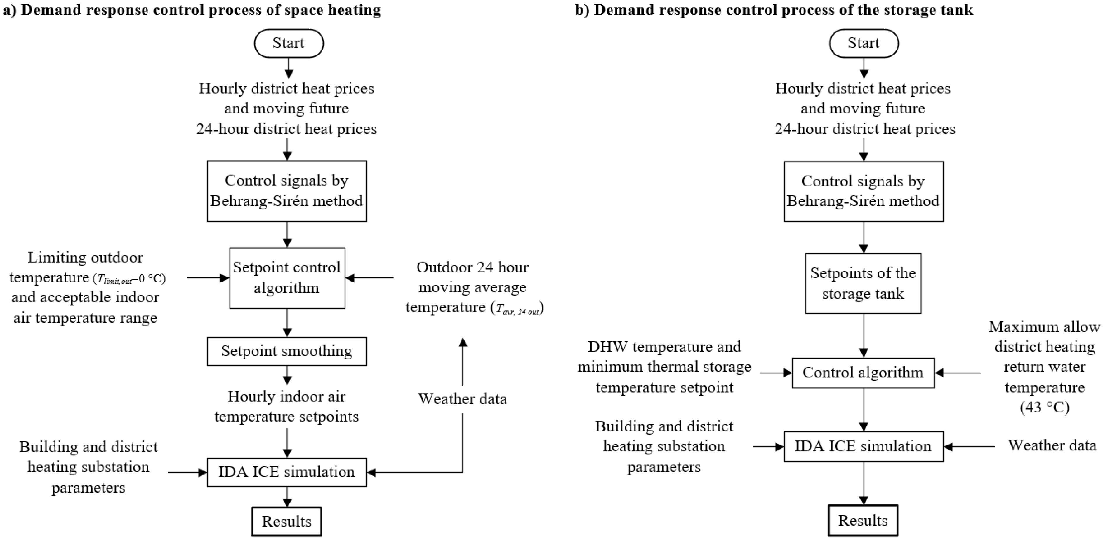
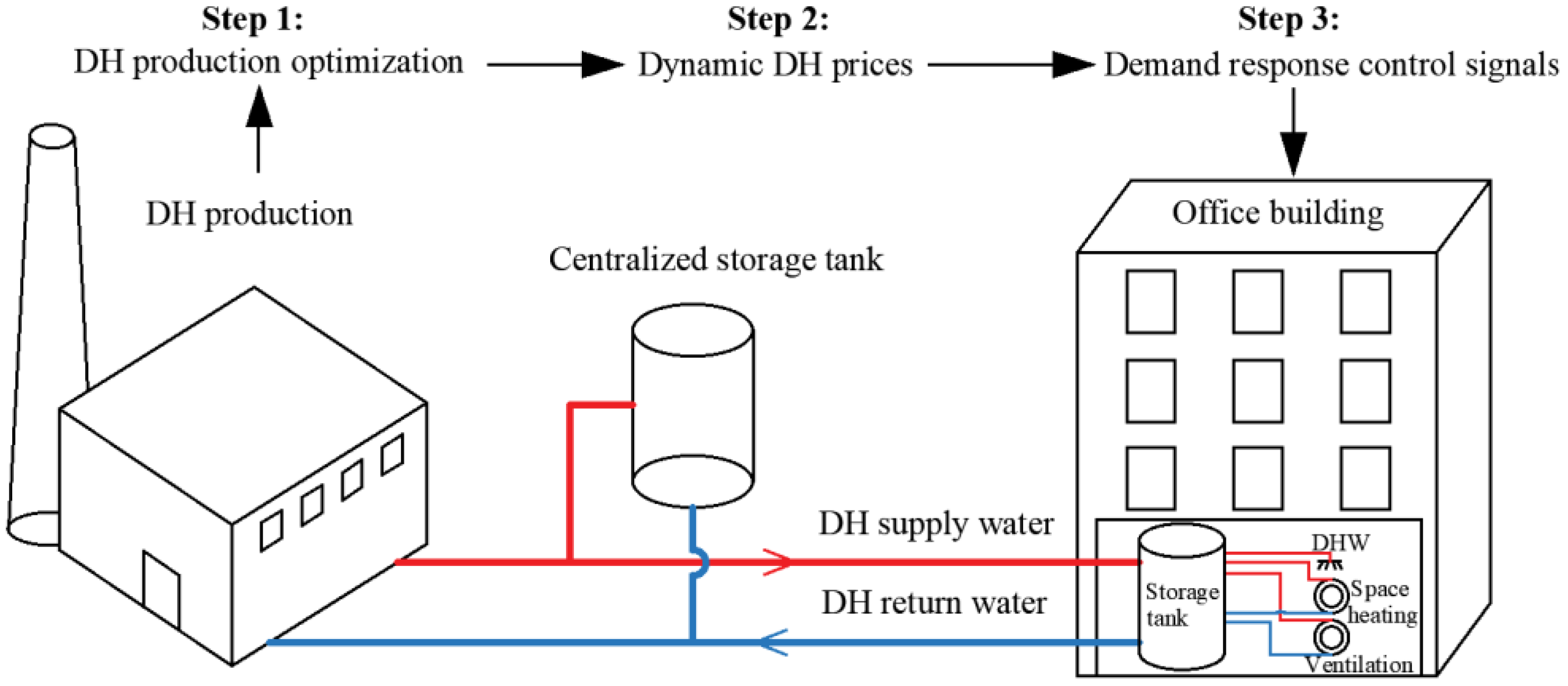
2.1. Description of the Simulation Process
2.2. DH Production
2.2.1. DH Network Modeling
2.2.2. Simulated DH System
2.2.3. District Heat Prices
2.2.4. Power Fee
2.3. Building Level Simulation
2.3.1. Simulated Building
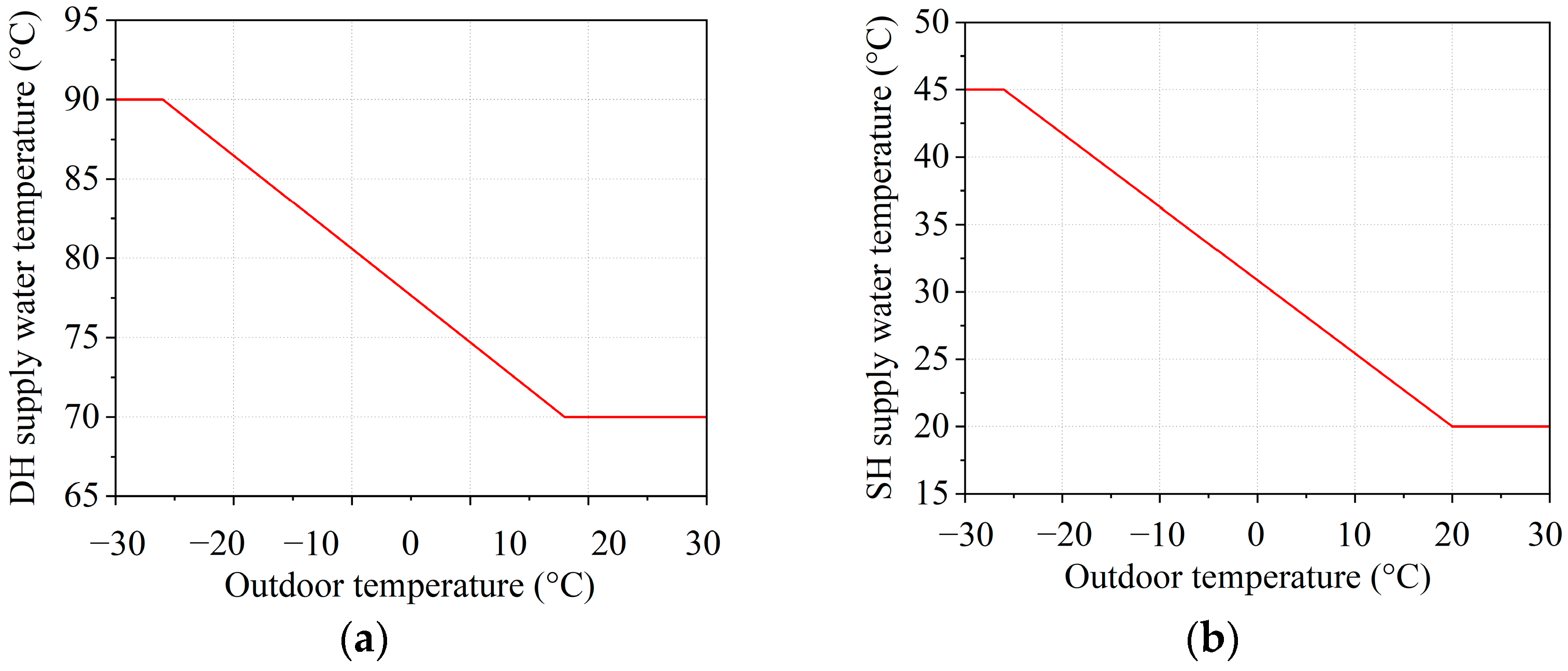
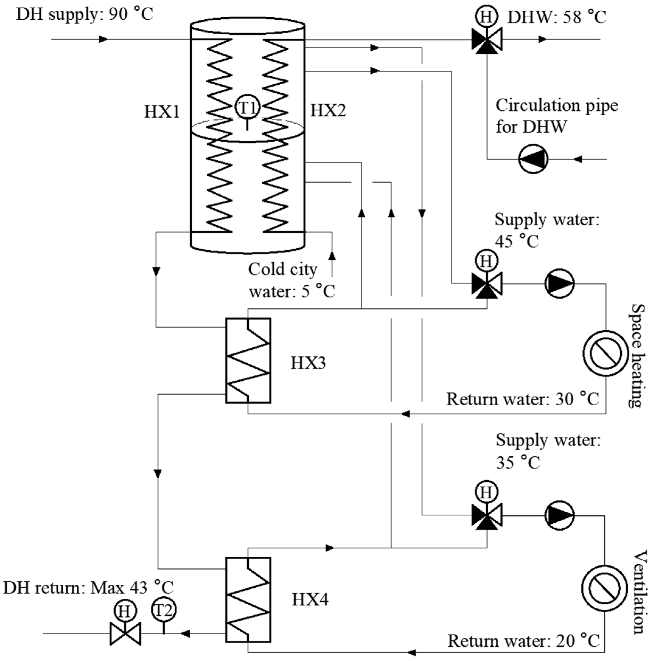
2.3.2. DH Substations
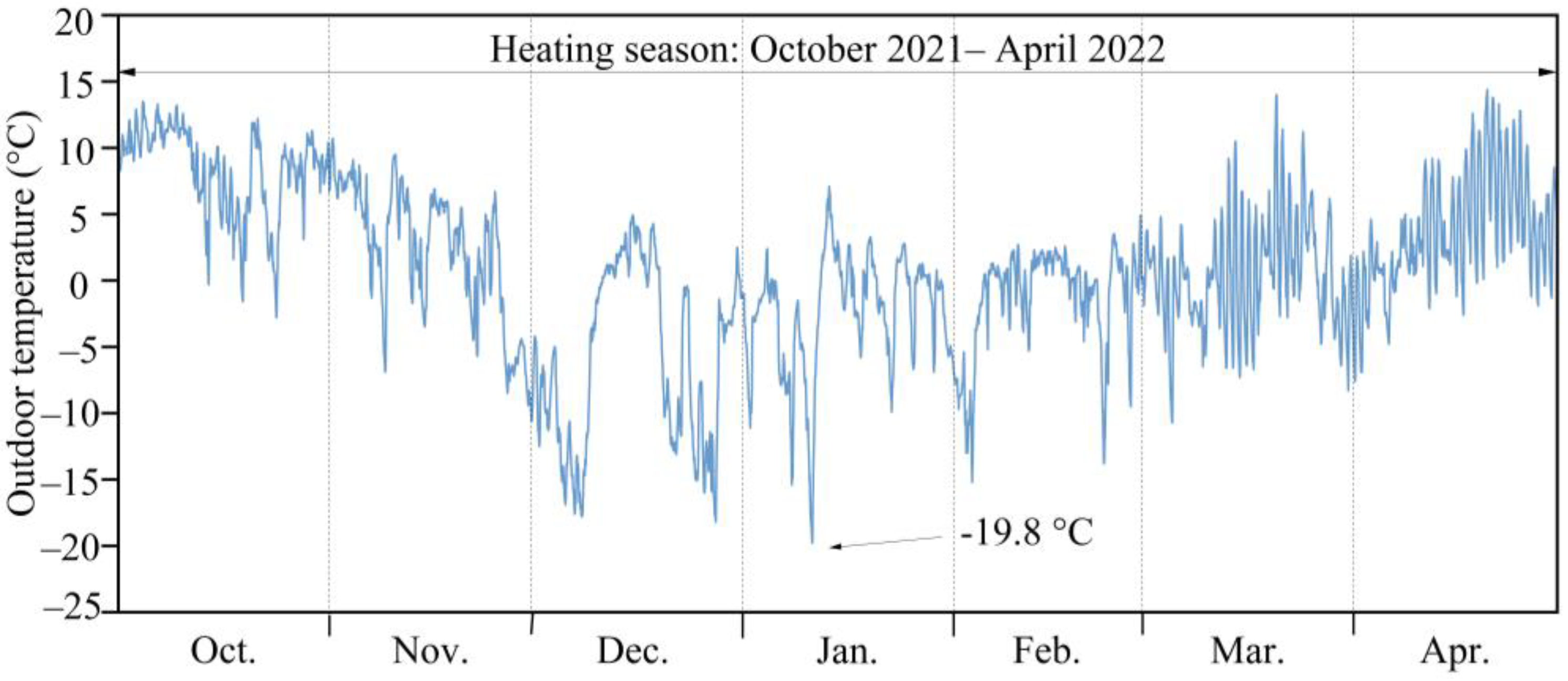
2.3.3. Simulation Tool and Weather Data
3. Demand Response Control Algorithms and Energy Flexibility
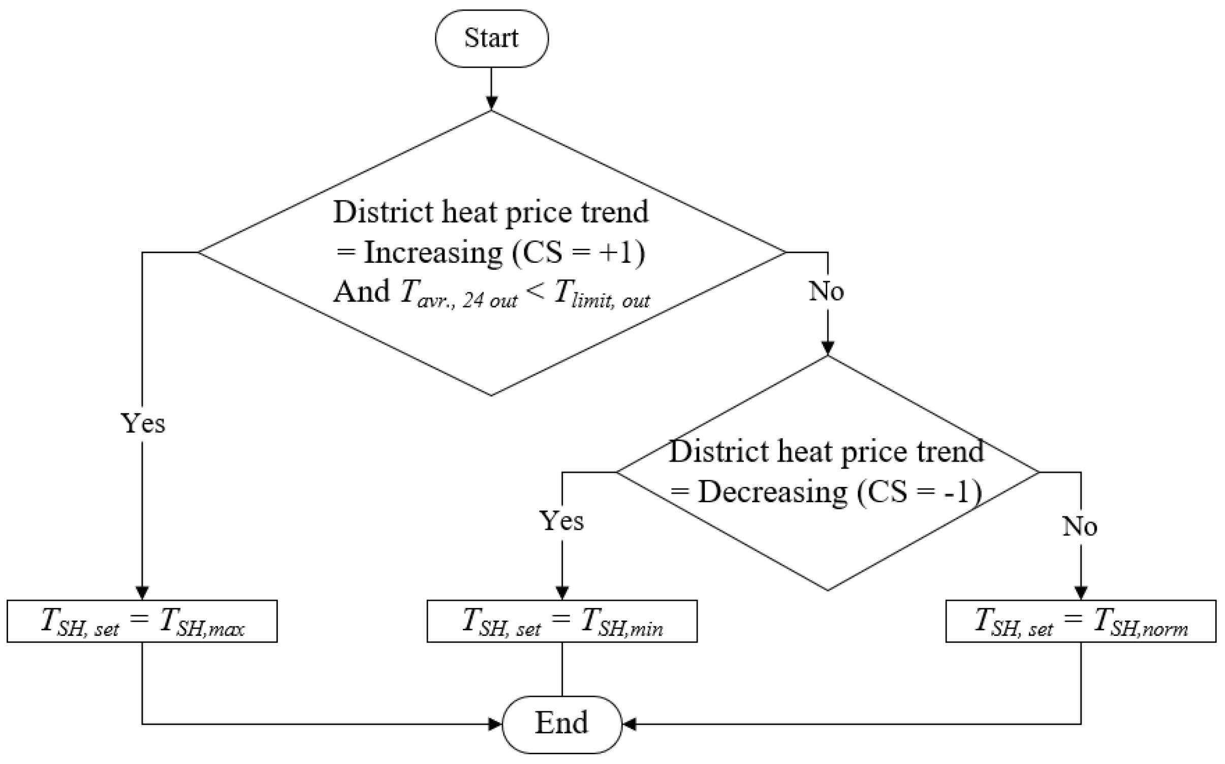
3.1. Demand Response Control Signals
3.2. Demand Response Control Algorithm of Space Heating
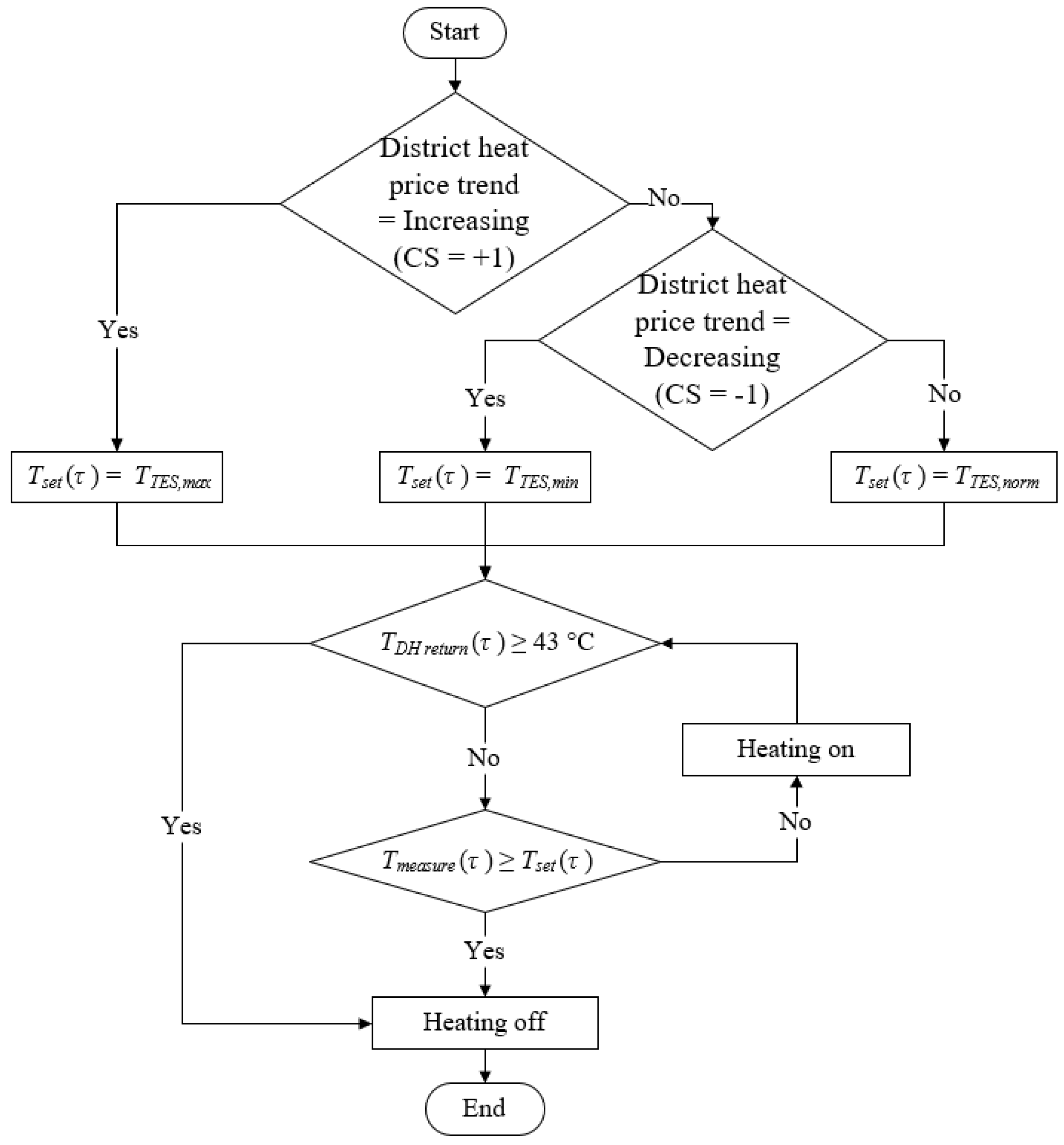
3.3. Demand Response Control Algorithm for the Thermal Storage Tank
3.4. Energy Flexibility Factors
3.5. Description of Simulated Cases
4. Results
4.1. Heat Energy Consumption, Costs, and Power Fee
4.2. Energy Flexibility
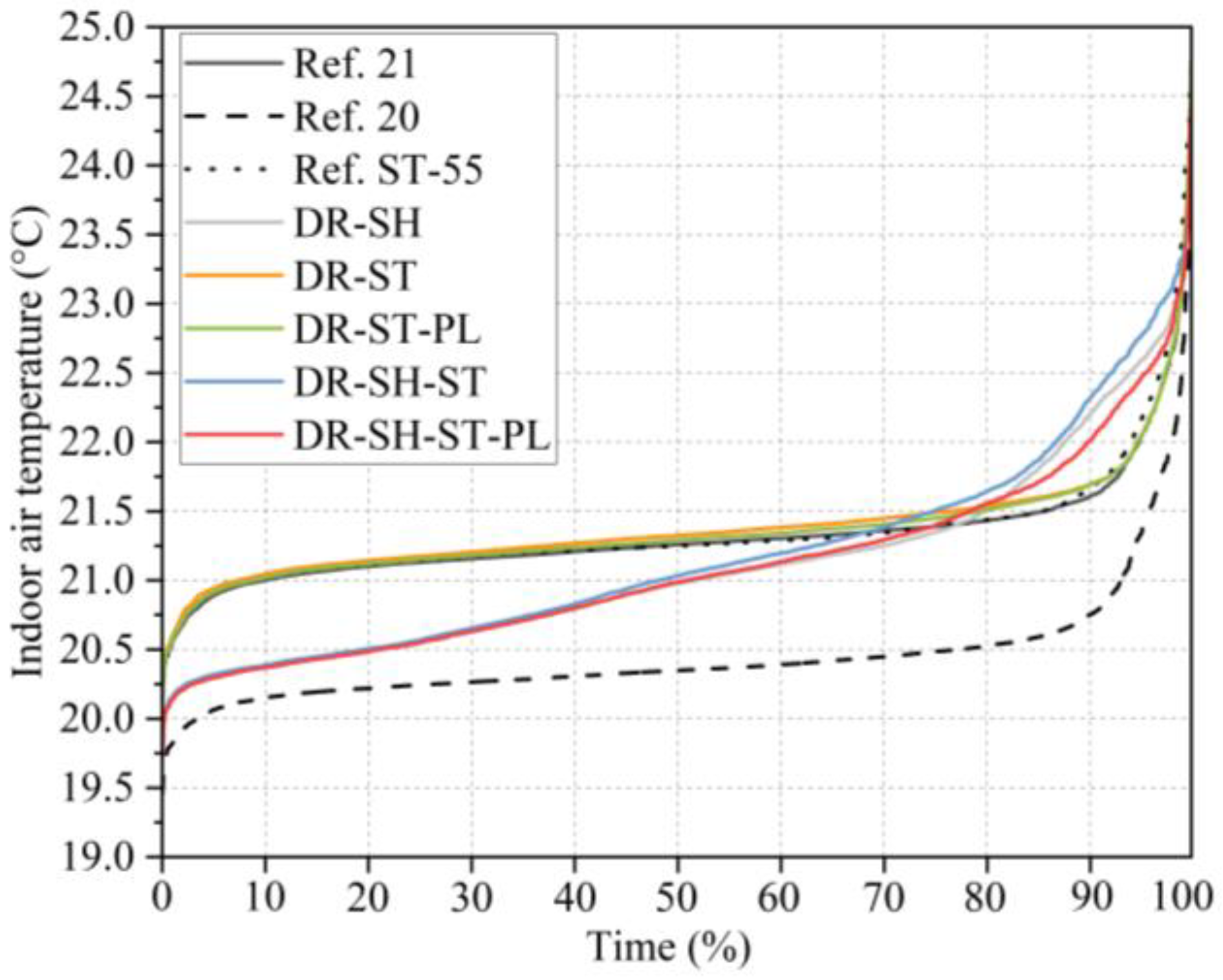
4.3. Indoor Air Temperature and Ventilation Conditions
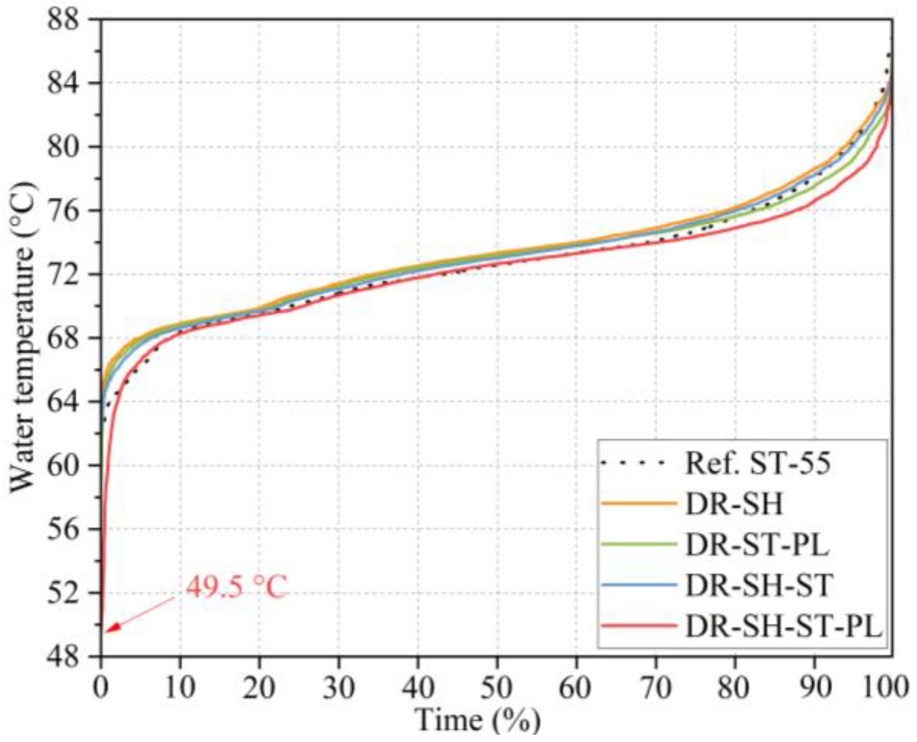
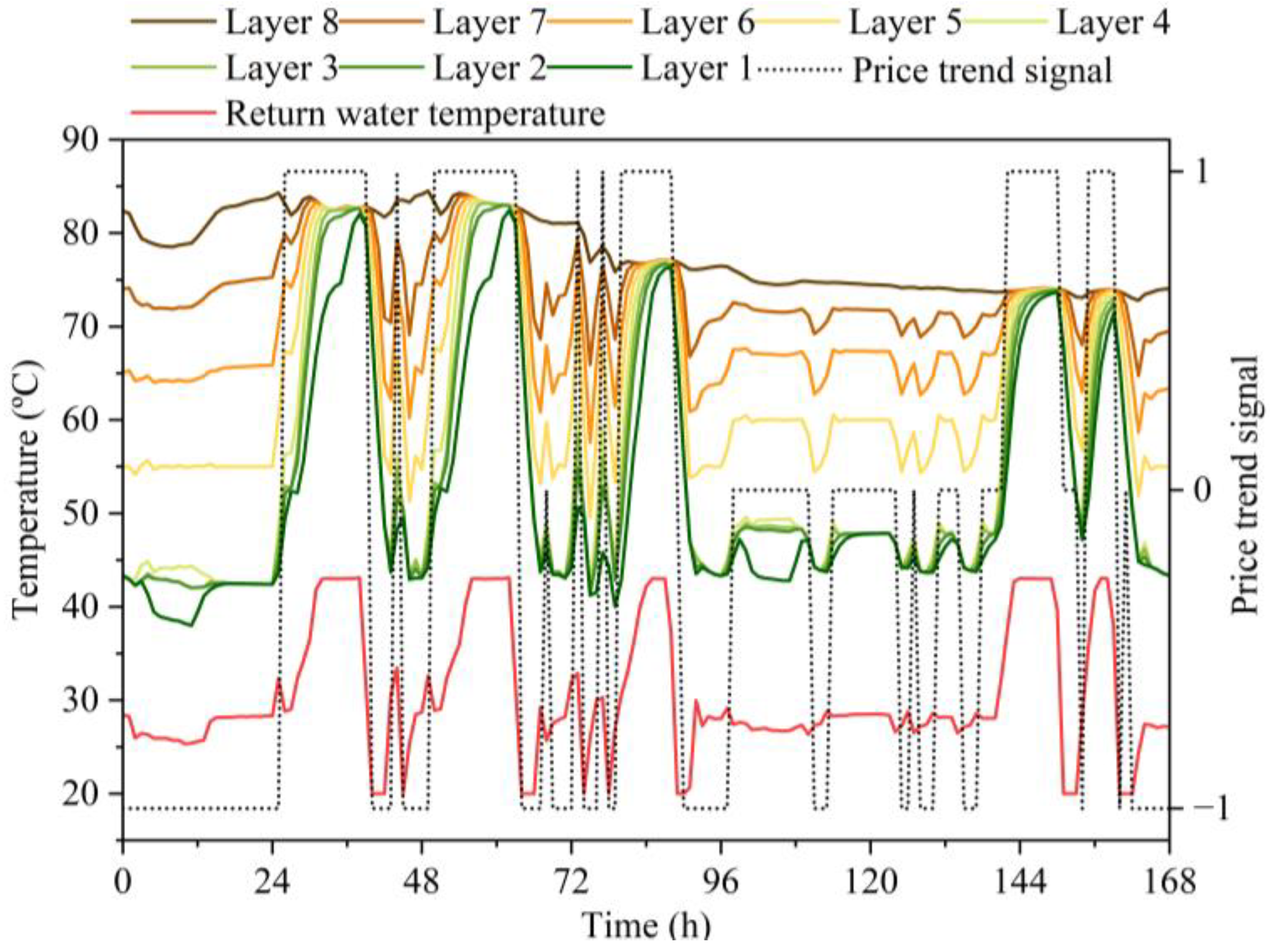
4.4. DHW Temperature and Tank Temperature
5. Discussion
6. Conclusions
Author Contributions
Funding
Data Availability Statement
Acknowledgments
Conflicts of Interest
References
- Finnish Energy. Energy Year 2022—District Heating. Available online: http://energia.fi/en/newsroom/publications/energy_year_2022_-_district_heating.html#material-view (accessed on 3 May 2023).
- Finnish Government. Programme of Prime Minister Sanna Marin’s Government 10 December 2019. Inclusive and Competent Finland—A Socially, Economically and Ecologically Sustainable Society. Available online: http://urn.fi/URN:ISBN:978-952-287-811-3 (accessed on 1 July 2021).
- Gelazanskas, L.; Gamage, K.A. Demand side management in smart grid: A review and proposals for future direction. Sustain. Cities Soc. 2014, 11, 22–30. [Google Scholar] [CrossRef]
- Ju, Y.; Lindholm, J.; Verbeck, M.; Jokisalo, J.; Kosonen, R.; Janßen, P.; Li, Y.; Kosonen, R.; Schäfers, H.; Nord, N. Cost savings and CO2 emissions reduction potential in the German district heating system with demand response. Sci. Technol. Built Environ. 2022, 28, 255–274. [Google Scholar] [CrossRef]
- Le Dréau, J.; Heiselberg, P. Energy flexibility of residential buildings using short term heat storage in the thermal mass. Energy 2016, 111, 991–1002. [Google Scholar] [CrossRef]
- Reynders, G.; Diriken, J.; Saelens, D. Generic characterization method for energy flexibility: Applied to structural thermal storage in residential buildings. Appl. Energy 2017, 198, 192–202. [Google Scholar] [CrossRef]
- Hedegaard, R.E.; Kristensen, M.H.; Pedersen, T.H.; Brun, A.; Petersen, S. Bottom-up modelling methodology for urban-scale analysis of residential space heating demand response. Appl. Energy 2019, 242, 181–204. [Google Scholar] [CrossRef]
- Dominković, D.F.; Gianniou, P.; Münster, M.; Heller, A.; Rode, C. Utilizing thermal building mass for storage in district heating systems: Combined building level simulations and system level optimization. Energy 2018, 153, 949–966. [Google Scholar] [CrossRef]
- Guelpa, E.; Verda, V. Thermal energy storage in district heating and cooling systems: A review. Appl. Energy 2019, 252, 113474. [Google Scholar] [CrossRef]
- Buffa, S.; Fouladfar, M.H.; Franchini, G.; Lozano Gabarre, I.; Andrés Chicote, M. Advanced control and fault detection strategies for district heating and cooling systems—A review. Appl. Sci. 2021, 11, 455. [Google Scholar] [CrossRef]
- Jebamalai, J.M.; Marlein, K.; Laverge, J. Influence of centralized and distributed thermal energy storage on district heating network design. Energy 2020, 202, 117689. [Google Scholar] [CrossRef]
- Rämä, M.; Wahlroos, M. Introduction of new decentralised renewable heat supply in an existing district heating system. Energy 2018, 154, 68–79. [Google Scholar] [CrossRef]
- Golmohamadi, H.; Larsen, K.G.; Jensen, P.G.; Hasrat, I.R. Integration of flexibility potentials of district heating systems into electricity markets: A review. Renew. Sustain. Energy Rev. 2022, 159, 112200. [Google Scholar] [CrossRef]
- Benalcazar, P. Optimal sizing of thermal energy storage systems for CHP plants considering specific investment costs: A case study. Energy 2021, 234, 121323. [Google Scholar] [CrossRef]
- Tan, J.; Wu, Q.; Zhang, M. Strategic investment for district heating systems participating in energy and reserve markets using heat flexibility. Int. J. Electr. Power Energy Syst. 2022, 137, 107819. [Google Scholar] [CrossRef]
- Doračić, B.; Pavičević, M.; Pukšec, T.; Duić, N. Bidding strategies for excess heat producers participating in a local wholesale heat market. Energy Rep. 2022, 8, 3692–3703. [Google Scholar] [CrossRef]
- Moser, S.; Puschnigg, S.; Rodin, V. Designing the Heat Merit Order to determine the value of industrial waste heat for district heating systems. Energy 2020, 200, 117579. [Google Scholar] [CrossRef]
- Liu, W.; Klip, D.; Zappa, W.; Jelles, S.; Kramer, G.J.; van den Broek, M. The marginal-cost pricing for a competitive wholesale district heating market: A case study in the Netherlands. Energy 2019, 189, 116367. [Google Scholar] [CrossRef]
- Cai, H.; Ziras, C.; You, S.; Li, R.; Honoré, K.; Bindner, H.W. Demand side management in urban district heating networks. Appl. Energy 2018, 230, 506–518. [Google Scholar] [CrossRef]
- Arabkoohsar, A. Non-uniform temperature district heating system with decentralized heat pumps and standalone storage tanks. Energy 2019, 170, 931–941. [Google Scholar] [CrossRef]
- Armstrong, P.; Ager, D.; Thompson, I.; McCulloch, M. Domestic hot water storage: Balancing thermal and sanitary performance. Energy Policy 2014, 68, 334–339. [Google Scholar] [CrossRef]
- FINLEX. Ympäristöministeriön Asetus Rakennusten Vesi- Ja Viemärilaitteistoista (Decree 1047/2017 Ministry of the Environment’s Decree on Water and Sewage Systems in Buildings). Available online: https://www.finlex.fi/fi/laki/alkup/2017/20171047 (accessed on 4 June 2023).
- Buffa, S.; Soppelsa, A.; Pipiciello, M.; Henze, G.; Fedrizzi, R. Fifth-generation district heating and cooling substations: Demand response with artificial neural network-based model predictive control. Energies 2020, 13, 4339. [Google Scholar] [CrossRef]
- Knudsen, M.D.; Petersen, S. Model predictive control for demand response of domestic hot water preparation in ultra-low temperature district heating systems. Energy Build. 2017, 146, 55–64. [Google Scholar] [CrossRef]
- Difs, K.; Trygg, L. Pricing district heating by marginal cost. Energy Policy 2009, 37, 606–616. [Google Scholar] [CrossRef]
- EMD International A/S. “EnergyPRO”. Available online: https://www.emd.dk/energypro/. (accessed on 10 February 2020).
- Nordpool. “Historical Market Data”. Available online: https://www.nordpoolgroup.com/historical-market-data/ (accessed on 1 October 2021).
- Finnish Energy Ltd. “Kaukolämpötilasto 2019 (Document in Finnish: District Heating in Finland 2019)”. Available online: https://energia.fi/files/5384/Kaukolampotilasto_2019.pdf (accessed on 9 December 2021).
- Helen Ltd. “Käyttöveden Lämmityksen Hinta (The Price of Hot Water Heating)”. Available online: https://www.helen.fi/lammitys-ja-jaahdytys/kaukolampo/hinnat/kayttoveden-lammityksen-hinta (accessed on 21 September 2023).
- Finnish Meteorological Institute. Lämmitystarveluku eli Astepäiväluku (Heating Demand Figure, i.e., Degree Day Figure). Available online: https://www.ilmatieteenlaitos.fi/lammitystarveluvut (accessed on 18 September 2023).
- energyPRO. User’guide. Available online: https://www.emd-international.com/energyPRO/Tutorials%20and%20How%20To%20Guides/energyPROHlpEng-4.5%20Nov.%2017.pdf (accessed on 21 September 2023).
- Fortum—Utilising Waste Heat with 2 Unitop 50 FY Heat Pumps. Available online: https://www.friotherm.com/wp-content/uploads/2017/11/E10-15_Suomenoja.pdf (accessed on 21 September 2023).
- Caruna, O. Suurjännitteisen Jakeluverkon Verkkopalvelu-Ja Liittymismaksuhinnasto. 1 February 2021. Available online: https://images.caruna.fi/31575610_caruna_liittymismaksuhinnasto_suurjannite_6s_fi_saavutettava.pdf. (accessed on 9 December 2021).
- Trading Economics. EU Carbon Permits. Available online: https://tradingeconomics.com/commodity/carbon (accessed on 9 December 2021).
- Tilastokeskus. Polttoaineluokitus (Fuel Calssification). Available online: https://www.stat.fi/tup/khkinv/khkaasut_.polttoaineluokitus.html (accessed on 19 August 2023).
- Fortum Ltd. Kaukolämmön Hinnat Taloyhtiöille Ja Yrityksille (District Heating Prices for Building Societies and Companies). Available online: https://www.fortum.fi/yrityksille-ja-yhteisoille/lammitys-ja-jaahdytys/kaukolampo/kaukolammon-hinnat-taloyhtioille-ja-yrityksille (accessed on 15 December 2022).
- SFS-EN 16798-1:2019; Energy Performance of Buildings. Ventilation for Buildings. Part 1: Indoor Environmental Input Parameters for Design and Assessment of Energy Performance of Buildings Addressing Indoor Air Quality, Thermal Environment, Lighting and Acoustics. Module M1-6. Finnish Standards Association (SFS): Helsinki, Finland, 2019.
- Suhonen, J.; Jokisalo, J.; Kosonen, R.; Kauppi, V.; Ju, Y.; Janßen, P. Demand response control of space heating in three different building types in Finland and Germany. Energies 2020, 13, 6296. [Google Scholar] [CrossRef]
- Ju, Y.; Jokisalo, J.; Kosonen, R.; Kauppi, V.; Janßen, P. Analyzing power and energy flexibilities by demand response in district heated buildings in Finland and Germany. Sci. Technol. Built Environ. 2021, 27, 1440–1460. [Google Scholar] [CrossRef]
- Ministry of the Environment. D3 Finnish Code of Building Regulation. Rakennusten Energiatehokkuus (Energy Efficiency of Buildings). Regulations and Guidelines; Ministry of the Environment: Helsinki, Finland, 1985. (In Finnish)
- Ministry of Environment. Decree of the Ministry of the Environment on the Indoor Climate and Ventilation of New Buildings. Ministry of Environment. Helsinki. Finland. Available online: https://ym.fi/documents/1410903/35099218/Indoor+Climate+and+Ventilation+of+New+Buildings.pdf/df12cdbf-a038-19cb-4dc6-254c6cc4f1be/Indoor+Climate+and+Ventilation+of+New+Buildings.pdf?t=1680607494788 (accessed on 9 July 2023).
- SFS-EN-ISO 7730; Ergonomics of the Thermal Environment. Analytical Determination and Interpretation of Thermal Comfort Using Calculation of the PMV and PPD Indices and Local Thermal Comfort Criteria. Finnish Standards Association: Helsinki, Finland, 2006.
- FINVAC (The Finnish Association of HVAC Societies). Opas Ilmanvaihdon Mitoitukseen Muissa Kuin Asuinrakennuksissa (The Guidelines of Ventilation Dimensioning in Other Buildings than Apartment Building). FINVAC. Available online: https://finvac.org/wp-content/uploads/2020/06/Opas_ilmanvaihdon_mitoitukseen_muissa_kuin_asuinrakennuksissa_2017.pdf (accessed on 20 March 2020). (In Finnish).
- EN 13779:2007; Ventilation for Non-Residential Buildings–Performance Requirements for Ventilation and Room-Conditioning Systems. The European Committee for Standardization (CEN): Brussels, Belgium, 2007.
- Publication K1/2021. Rakennusten kaukolämmitys-Määräykset ja Ohjeet-Julkaisu K1/2021(District Heating of Buildings-Regulations and Guidelines-Publication K1/2021). Energiateollisuus. Available online: https://lnkd.in/gsyNvwk2 (accessed on 12 August 2022). (In Finnish).
- Sahlin, P. Modelling and Simulation Methods for Modular Continuous Systems in Buildings. Ph.D. Thesis, Royal Institute of Technology, Stockholm, Sweden, 1996. Available online: https://www.equa.se/dncenter/thesis.pdf (accessed on 2 March 2020).
- EQUA Simulation Technology Group. Validation of IDA Indoor Climate and Energy 4.0 with Respect to CEN Standards EN 15255-2007 and EN 15265-2007; EQUA Simulation Technology Group: 2010. Available online: http://www.equaonline.com/iceuser/CEN_VALIDATION_EN_15255_AND_15265.pdf (accessed on 11 February 2023).
- Bring, A.; Sahlin, P.; Vuolle, M. Models for Building Indoor Climate and Energy Simulation—A Report of IEA SHC Task 22: Building Energy Analysis Tools; IEA: Stockholm, Sweden, 1999. [Google Scholar]
- EQUA Simulation Technology Group. Validation of IDA Indoor Climate and Energy 4.0 Build 4 with Respect to ANSI/ASHRAE Standard 140-2004, EQAU Simulation Technology Group: 2010. Available online: http://www.equaonline.com/iceuser/validation/ASHRAE140-2004.pdf (accessed on 11 February 2023).
- Moosberger, S. IDA ICE CIBSE-Validation: Test of IDA Indoor Climate and Energy Version 4.0 according to CIBSE TM33, Issue 3. HTA LUZRN/ZIG: 2007. Available online: http://www.equaonline.com/iceuser/validation/ICE-Validation-CIBSE_TM33.pdf (accessed on 11 February 2023).
- Verda, V.; Colella, F. Primary energy savings through thermal storage in district heating networks. Energy 2011, 36, 4278–4286. [Google Scholar] [CrossRef]
- Ju, Y.; Jokisalo, J.; Kosonen, R. Peak Shaving of a District Heated Office Building with Short-Term Thermal Energy Storage in Finland. Buildings 2023, 13, 573. [Google Scholar] [CrossRef]
- Alimohammadisagvand, B.; Jokisalo, J.; Kilpeläinen, S.; Ali, M.; Sirén, K. Cost-optimal thermal energy storage system for a residential building with heat pump heating and demand response control. Appl. Energy 2016, 174, 275–287. [Google Scholar] [CrossRef]
- Finnish Meteorological Institute. Weather and Sea—Download Observations. Available online: https://en.ilmatieteenlaitos.fi/download-observations (accessed on 28 January 2023).
- Martin, K. Demand Response of Heating and Ventilation within Educational Office Buildings. Master’s Thesis, Aalto University, School of Engineering, Department of Energy Technology, HVAC, Espoo, Finland, 2017. Available online: https://aaltodoc.aalto.fi/handle/123456789/29149 (accessed on 4 March 2021).
- Li, H.; Svendsen, S.; Gudmundsson, O.; Kuosa, M.; Rämä, M.; Sipilä, K.; Blesl, M.; Broydo, M.; Stehle, M.; Pesch, R.; et al. Annex TS1 Low Temperature District Heating for Future Energy Systems—Final Report—Future Low Temperature District Heating Design Guidebook. Int. Energy Agency 2017. Available online: https://core.ac.uk/download/pdf/154332407.pdf (accessed on 11 February 2023).
- Tabatabaei, S.A.; Klein, M. The role of knowledge about user behaviour in demand response management of domestic hot water usage. Energy Effic. 2018, 11, 1797–1809. [Google Scholar] [CrossRef]
- Alimohammadisagvand, B.; Alam, S.; Ali, M.; Degefa, M.; Jokisalo, J.; Sirén, K. Influence of energy demand response actions on thermal comfort and energy cost in electrically heated residential houses. Indoor Built Environ. 2017, 26, 298–316. [Google Scholar] [CrossRef]


| Thermal Capacity (MW) | DH Supply Temperature (°C) | DH Return Temperature (°C) | Heat Source Inlet Temperature (°C) | Heat Source Outlet Temperature (°C) | COP |
|---|---|---|---|---|---|
| 47 | 65 | 50 | 14 | 7 | 3.7 |
| Unit | Fuel Type | Fuel Capacity (MW) | Generated Heat (MW) | Generated Electricity (MW) |
|---|---|---|---|---|
| CHP 1 | Coal | 265 | 160 | 80 |
| CHP 2 | Natural gas | 498 | 214 | 234 |
| CHP 3 | Natural gas | 132 | 75 | 45 |
| Heat-only boiler (HOB) 1 | Natural gas | 496 | 446 | - |
| Heat-only boiler (HOB) 2 | Light fuel oil | 94 | 85 | - |
| Heat-only boiler (HOB) 3 | Wood pellet | 90 | 80 | - |
| Heat-only boiler (HOB) 4 | Bio oil | 98 | 90 | - |
| Heat-only boiler (HOB) 5 | Wood chip | 49 | 52 | - |
| Heat pump (HP) | - | - | 47 | - |
| Type of the Fee | Price (€/MWh) |
|---|---|
| Spot price | Average: 136.42 |
| Distribution fee, winter days (7 a.m.–9 p.m., 1.12–28.2) [33] | 9.91 |
| Distribution fee, other time [33] | 3.29 |
| Electricity tax and security of supply fee (€/MWh) | 22.53 |
| Load fee, intake from the grid (€/MWh) | 1.81 |
| Load fee, output to the grid (€/MWh) | 0.76 |
| Fuel Type | Fuel Price (€/MWh) | Fuel Tax of Heat-Only Boiler (HOB) (€/MWh) | Fuel Tax of CHP (€/MWh) | Emission Factor [35] (tonCO2/MWh) |
|---|---|---|---|---|
| Coal | 22.81 | 32.00 | 24.34 | 0.335 |
| Natural gas | 97.13 | 23.35 | 15.72 | 0.199 |
| Light fuel oil | 149.78 | 30.21 | - | 0.255 |
| Wood pellet | 46.00 | - | - | - |
| Wood chip | 24.23 | - | - | - |
| Bio oil | 67.00 | 10.67 | - | - |
| Parameters | Office Building |
|---|---|
| Heated net floor area (m2) | 2383 |
| Floor number | 4 |
| Envelope area (m2) | 3855 |
| Window/envelope area | 9.5% |
| U-Value of external walls [40] (W/m2·K) | 0.28 |
| U-Value of roof [40] (W/m2·K) | 0.22 |
| U-Value of ground slab [40] (W/m2·K) | 0.36 |
| U-Value of windows [40] (W/m2·K) | 1.00 |
| Air leakage rate, n50 (1/h) | 1.60 |
| Usage time | 8 a.m.–4 p.m. (workdays) |
| Annual internal heat gains of equipment (kWh/m2·a) | 3.7 |
| Annual internal heat gains of lighting (kWh/m2·a) | 18.3 |
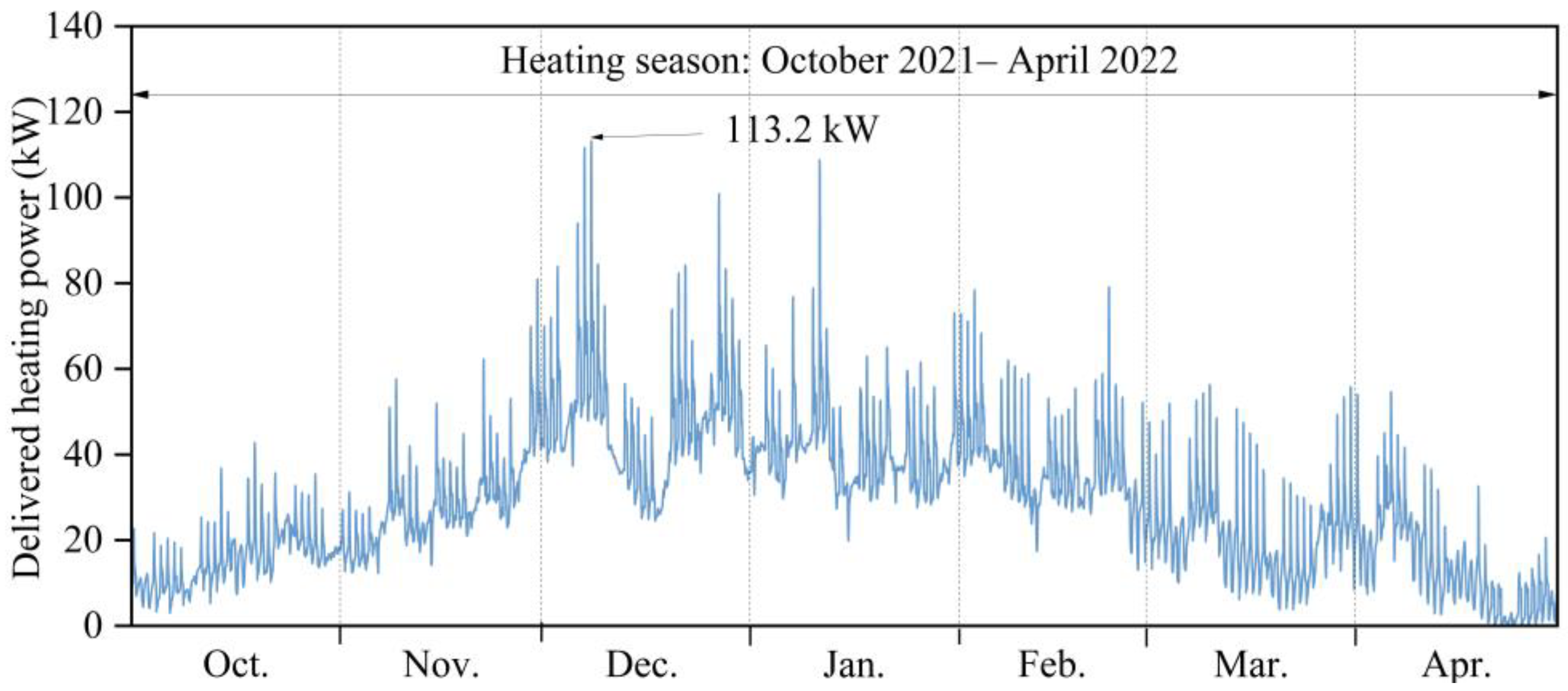
| Actual peak heating power demand (kW) | 113.2 |
| Ventilation System | Airflow Rates [43] | Operation Time |
|---|---|---|
| Mechanical supply and exhaust ventilation (VAV with CO2 control) with 65% heat recovery for meeting rooms | 0.35–3 L/s, m2 | 6 a.m.–6 p.m. for workdays |
| Mechanical supply and exhaust ventilation (CAV) with 65% heat recovery for office rooms and hallway | 0.35–1.5 L/s, m2 |
| Price Trend | Increasing | Decreasing | Flat |
|---|---|---|---|
| Average district heat price (€/MWh) | 57.1 | 94.4 | 62.9 |
| Cases | Indoor Air Temperature Setpoint (°C) | Storage Tank Temperature Setpoint (°C) | Substation | DR of Space Heating | DR of Thermal Storage Tank | Peak Power Limiting |
|---|---|---|---|---|---|---|
| Ref. 21 | 21 | -- | 1 | -- | -- | -- |
| Ref. 20 | 20 | -- | 1 | -- | -- | -- |
| Ref. ST-55 | 21 | 55 | 2 | -- | -- | -- |
| DR-SH | 20–23 | -- | 1 | √ | -- | -- |
| DR-ST | 21 | 55–90 1 | 2 | -- | √ | -- |
| DR-ST-PL | 21 | 55–90 | 2 | -- | √ | √ |
| DR-SH-ST | 20–23 | 55–90 | 2 | √ | √ | -- |
| DR-SH-ST-PL | 20–23 | 55–90 | 2 | √ | √ | √ |
| Cases | Max Heating Power (kW) | Heat Energy Consumption | District Heat Energy Cost | Power Fee | Total Cost | ||||
|---|---|---|---|---|---|---|---|---|---|
| kWh/m2 | Diff. | €/m2 | Diff. | €/m2 | Diff. | €/m2 | Diff. | ||
| Ref. 21 | 113.2 | 61.5 | 5.00 | 3.47 | 8.47 | ||||
| Ref. 20 | 111.8 | 57.6 | −6.2% | 4.70 | −6.0% | 3.43 | −1.2% | 8.13 | −4.0% |
| Ref. ST-55 | 108.3 | 61.4 | −0.2% | 4.93 | −1.4% | 3.33 | −4.0% | 8.26 | −2.5% |
| DR-SH | 112.8 | 60.6 | −1.4% | 4.52 | −9.6% | 3.45 | −0.6% | 7.97 | −5.9% |
| DR-ST | 112.4 | 62.6 | 1.9% | 4.83 | −3.4% | 3.44 | −0.9% | 8.27 | −2.4% |
| DR-ST-PL | 64.2 | 62.4 | 1.5% | 4.85 | −3.0% | 2.04 | −41.2% | 6.89 | −18.7% |
| DR-SH-ST | 112.4 | 61.7 | 0.4% | 4.36 | −12.8% | 3.44 | −0.9% | 7.80 | −7.9% |
| DR-SH-ST-PL | 64.2 | 61.2 | −0.4% | 4.53 | −9.4% | 2.04 | −41.2% | 6.57 | −22.4% |
| Setpoints (°C) | Indoor Air Temperature | Building-Level Storage Tank | ||||
|---|---|---|---|---|---|---|
| Discharging (Min 20) | Normal 21 | Charging (Max 23) | Discharging (Min 55) | Normal 60 | Charging (Max 90) | |
| Number of hours | 2393 | 2123 | 573 | 2393 | 1623 | 1073 |
| Total | 5089 | 5089 | ||||
| Cases | DR-SH | DR-ST | DR-ST-PL | DR-SH-ST | DR-SH-ST-PL |
|---|---|---|---|---|---|
| FF+ | 10.3% | 8.4% | 7.5% | 19.0% | 12.5% |
| FF− | −14.2% | −4.6% | −4.3% | −19.3% | −15.9% |
| Cases | Hours below (h) | Degree Hours below (°Ch) | ||
|---|---|---|---|---|
| 20 °C | 21 °C | 20 °C | 21 °C | |
| Ref. 21 | 0 | 354 | 0 | 86 |
| Ref. 20 | 126 | 4725 | 22 | 3113 |
| Ref. ST-55 | 0 | 279 | 0 | 71 |
| DR-SH | 7 | 2457 | 2 | 1082 |
| DR-ST | 0 | 268 | 0 | 64 |
| DR-ST-PL | 0 | 313 | 0 | 76 |
| DR-SH-ST | 6 | 2324 | 1 | 1026 |
| DR-SH-ST-PL | 7 | 2435 | 1 | 1089 |
Disclaimer/Publisher’s Note: The statements, opinions and data contained in all publications are solely those of the individual author(s) and contributor(s) and not of MDPI and/or the editor(s). MDPI and/or the editor(s) disclaim responsibility for any injury to people or property resulting from any ideas, methods, instructions or products referred to in the content. |
© 2023 by the authors. Licensee MDPI, Basel, Switzerland. This article is an open access article distributed under the terms and conditions of the Creative Commons Attribution (CC BY) license (https://creativecommons.org/licenses/by/4.0/).
Share and Cite
Ju, Y.; Hiltunen, P.; Jokisalo, J.; Kosonen, R.; Syri, S. Benefits through Space Heating and Thermal Storage with Demand Response Control for a District-Heated Office Building. Buildings 2023, 13, 2670. https://doi.org/10.3390/buildings13102670
Ju Y, Hiltunen P, Jokisalo J, Kosonen R, Syri S. Benefits through Space Heating and Thermal Storage with Demand Response Control for a District-Heated Office Building. Buildings. 2023; 13(10):2670. https://doi.org/10.3390/buildings13102670
Chicago/Turabian StyleJu, Yuchen, Pauli Hiltunen, Juha Jokisalo, Risto Kosonen, and Sanna Syri. 2023. "Benefits through Space Heating and Thermal Storage with Demand Response Control for a District-Heated Office Building" Buildings 13, no. 10: 2670. https://doi.org/10.3390/buildings13102670
APA StyleJu, Y., Hiltunen, P., Jokisalo, J., Kosonen, R., & Syri, S. (2023). Benefits through Space Heating and Thermal Storage with Demand Response Control for a District-Heated Office Building. Buildings, 13(10), 2670. https://doi.org/10.3390/buildings13102670