Abstract
Numerous studies have examined the responses of various structures to the mainshock–aftershock (MS–AS) ground motion, and the MS–AS ground motions are very important as the input. Therefore, in the absence of aftershock information, it is particularly critical to construct a reasonable MS–AS seismic sequence. This paper aims to provide a new reasonable method for generating the target aftershock response spectrum, which can be used to select or artificially simulate aftershock ground motion, given the seismic information of the main shock. Firstly, the magnitude, fault size, and location of the aftershock are determined. Then, other parameters required for the aftershock ground motion prediction equation (GMPE) are calculated. Subsequently, the correlation of the spectral shape to the MS–AS ground motion is used to modify the response spectrum predicted using the GMPE to obtain the conditional mean spectrum of aftershocks (CMSA). Finally, the relative errors of the predicted spectrum via the ASK14 model and CMSA are compared for four different assumptions. The results show that the simulated aftershock parameters and the actual ones accord well, and the relative errors of the CMSA can be controlled within 20%. Meanwhile, the discrete property of the target aftershock response spectrum is closer to the real recorded response spectrum.
1. Introduction
After an earthquake, many aftershocks often occur within a short period of time. Generally, the magnitude of aftershocks and their intensities are smaller than those of the main earthquake. However, the intensity of ground shaking caused by aftershocks at some sites may be greater than that of the main earthquake, such as the Christchurch aftershocks in New Zealand on 22 February 2011 [1]. Due to the randomness of various factors such as the focal location, focal depth, fault strike in the earthquake, and site conditions, the disaster caused by the aftershock is more catastrophic than the main earthquake. Therefore, some researchers have shifted more attention to the responses of various structures under the main shock and aftershocks [2,3,4,5,6,7], such as the special steel moment frame structures, corroded steel moment-resisting frames, etc. As a result, structural performance indexes such as vulnerability and recoverability under main shock and aftershock have been widely studied [8,9,10].
In studying structural reactions to MS–AS seismic sequences, researchers discovered that the input MS–AS ground motions significantly impact structural reactions. The most used types of MS–AS ground motions are repetitive and random ground motion sequences [11,12]. Torres et al. [13] improved the seismic performance of steel frames in MS–AS sequences, of which its aftershock ground motions were made by scaling the other mainshock ground motions. This method can reflect the relationship between the main shock and aftershocks in response spectrum amplitude to a certain extent. However, this method could be improved if the correlation and randomness of the main shock and aftershocks for the source mechanism, spectral shape, etc., are also considered. The same limitation was also observed in other studies [14]. Wei et al. [15] pointed out that the concrete-filled steel tubular composite columns with ultra-high performance concrete plates demonstrated good seismic performances with MS–AS sequences. If the above MS–AS sequences could reflect the correlation and randomness between the mainshock ground motions and their real aftershock ground motions, then the result might be more reasonable. For that reason, the real MS–AS ground motions were widely selected from different regional databases of strong motions [16] and then scaled to the target level based on local seismic hazards [17,18,19]. However, the real MS–AS ground motions may underestimate the aftershock impacts because the selected real seismic records cannot fully reflect the randomness of aftershock seismic sequences [20]. It may be difficult to fully reflect the randomness of the main shock and aftershocks in focal location, fault type, etc., for a small amount of real main shock and aftershock ground motions.
Therefore, it is necessary to construct an artificial main aftershock sequence to consider the correlation and randomness between the mainshock and aftershock ground motions [21,22]. Wang et al. [23] used the stochastic simulation of the main aftershock sequence to analyze the permanent displacement reliability of soil slopes based on the physical random function. The function could reflect the characteristics of the local site of the project by modeling the source, propagation path, and local site. The epidemic-type aftershock sequence (ETAS) model [24] and the branching aftershock sequence (BASS) model [25] are also widely used to simulate the regional aftershock sequences. Wang et al. [23] analyzed the stochastic simulation of the main aftershock sequences based on the physical random function and established the relationship between the main shock and aftershocks according to the theoretical copula model. The above method considers the correlation between some parameters of the main shock and aftershocks. Moreover, some researchers use an aftershock seismic hazard analysis to select ground tremors [26], which requires detailed seismic information. In recent years, some researchers [27] have begun to predict the parameters of aftershocks using machine learning methods, which may not fully explain the relevant mechanism.
This study strives to present a novel target aftershock spectrum that can, to the greatest extent feasible, capture the correlation and randomness between the MS–AS ground motions. The simulation approach fills in all the missing data for the GMPE of the aftershock ground motions based on the correlation and randomness between the main shock and its aftershocks, given the main earthquake. The aftershock magnitude and the hypocenter position should be established first to gather the necessary data. The location and size of aftershock faults are then estimated using the statistical relationship between magnitude and fault size and other relevant hypotheses. All other factors, including the rupture distance and hanging wall effect, are then calculated following their definitions. With the help of the aforementioned information, the GMPE was able to anticipate the response spectrum of the aftershock ground motions. On this foundation, it is possible to change the prediction spectrum of GMPE and achieve the target response spectrum of the aftershock using the prediction model of spectral shape parameters between the main shock and aftershocks. Therefore, this study could provide a new aftershock target response spectrum for studying high-performance concrete [28,29] and other structures subjected to the MS–AS seismic sequences.
2. The Target Aftershock Spectrum
The conditional mean spectrum of the aftershock (CMSA) is selected to generate the target aftershock spectrum given the mainshock ground motion. The CMSA could reflect the correlation of the spectral shapes between the mainshock ground motion and its aftershock ground motions. Given the response spectrum of the mainshock ground motion, the conditional mean of the response spectrum of the aftershock ground motion for the same period could be calculated as follows:
where MA and RA are the magnitude and source-to-site distance of an aftershock, respectively; Sa,A and Sa,M are the spectral accelerations of the aftershocks and their corresponding mainshock, respectively; and are the mean and standard deviation of lnSa,A predicted via the GMPE, respectively; εA and εM are the epsilon values of the aftershocks and their corresponding mainshock, respectively; is the conditional mean of conditioned on for the same period Ti,
where , , , and are the means and standard deviations of and for the period , respectively; is the correlation coefficient between and for the period . For more details regarding the values of the above parameters, interested readers are encouraged to refer to the work of Zhu et al. [30]. The exponent of is the conditional mean spectrum of aftershocks.
According to the above section, the CMSA is based on the GMPE of the aftershock and the correlation of the spectral shapes of the MS–AS ground motions. In this study, the ASK14 model [31] is selected to calculate the prediction spectrum of the aftershock ground motions because the ASK14 model could be used to predict the response spectrum of both mainshock and aftershock ground motions. Therefore, reasonably determining the aftershock seismic parameters for the ASK14 model becomes one of the key steps to calculating CMSA. Meanwhile, the complexity in calculating the conditional mean spectrum of aftershocks depends on how rich the parameters are for the aftershock ground motions, given the mainshock ground motions. The conditional mean spectrum of aftershocks can be calculated directly with all the required parameters of the aftershock ground motions. For example, the station for recording the ground motion is broken after the main shock. In this case, the aftershock ground motions are not recorded, but its seismic parameters are collected. However, the statistical relationship between the main shock and its aftershocks and the corresponding assumption can be used to supplement the missing data for regions with partially missing data from the aftershocks or where the data from the aftershocks is completely absent.
3. Determination of Aftershock Seismic Parameters
In proposing the conditional mean spectrum of aftershocks, the calculation procedure for generating CMSA is also provided in previous research [30]. Knowing how to reasonably determine the seismic parameters of the aftershock ground motions is an essential step, given the mainshock ground motions. This section will propose the method and assumptions for determining the seismic parameters of the aftershock ground motions based on the existing research results.
3.1. The Parameters Related to the Source
The mainshock is usually followed by a series of aftershocks, and only the maximum aftershock in terms of magnitude will be considered in this paper. The mean of the magnitude difference (Δm) between the mainshock and its largest aftershocks is about 1.2, and Δm ranges between about 0 and 3. Han et al. [32] point out that the beta distribution is the best candidate to describe the distribution of Δm. The beta distribution can be expressed as
where is the probability density function (PDF) of the selected beta distribution, as shown in Figure 1, in which is the beta function for the corresponding elements 2.2 and 2.3. With the distribution of Δm determined, the magnitude of the largest aftershock can be obtained by subtracting Δm from the mainshock magnitude.
Figure 1.
The probability density function of Δm.
The simplest assumption is that the aftershocks and its mainshock occur at the same place, but it will lead to bias [20]. Another assumption is that the epicenters of the aftershocks are uniformly distributed along the rupture length of the fault of their mainshock [33], as shown in Figure 2. Furthermore, it is also assumed that the epicenters of the aftershocks occur around the epicenter of their mainshock uniformly [34], as shown in Figure 3. The area of the circular region is related to the magnitude of their main shock and can be determined as follows:
where A is the area of the circular region (km2), and MM is the magnitude of their mainshock. With the determination of A, the radius of the circular region (R in Figure 3) can be calculated further.
Figure 2.
Hypocenter and rupture of the largest aftershock under linear assumption.
Figure 3.
Hypocenter and rupture of the largest aftershock under the circular assumption.
The depths of the hypocenters of the aftershocks are assumed to be the same as that of the mainshock, and the rupture planes of the aftershocks are parallel to the rupture plane of the mainshock. In other words, the strike angles and dip angles of the fault planes of the aftershocks are assumed to be the same as those of the mainshock. The size of the rupture plane of the aftershock can be determined as follows [35]:
where L and W are the rupture length and width, respectively. The coefficients a and b are listed in Table 1. LM and WM are the rupture length and width of the mainshock, and LA and WA are the rupture length and width of the aftershock, as shown in Figure 2 and Figure 3.
Table 1.
Regressions of the rupture length (L) and rupture width (W).
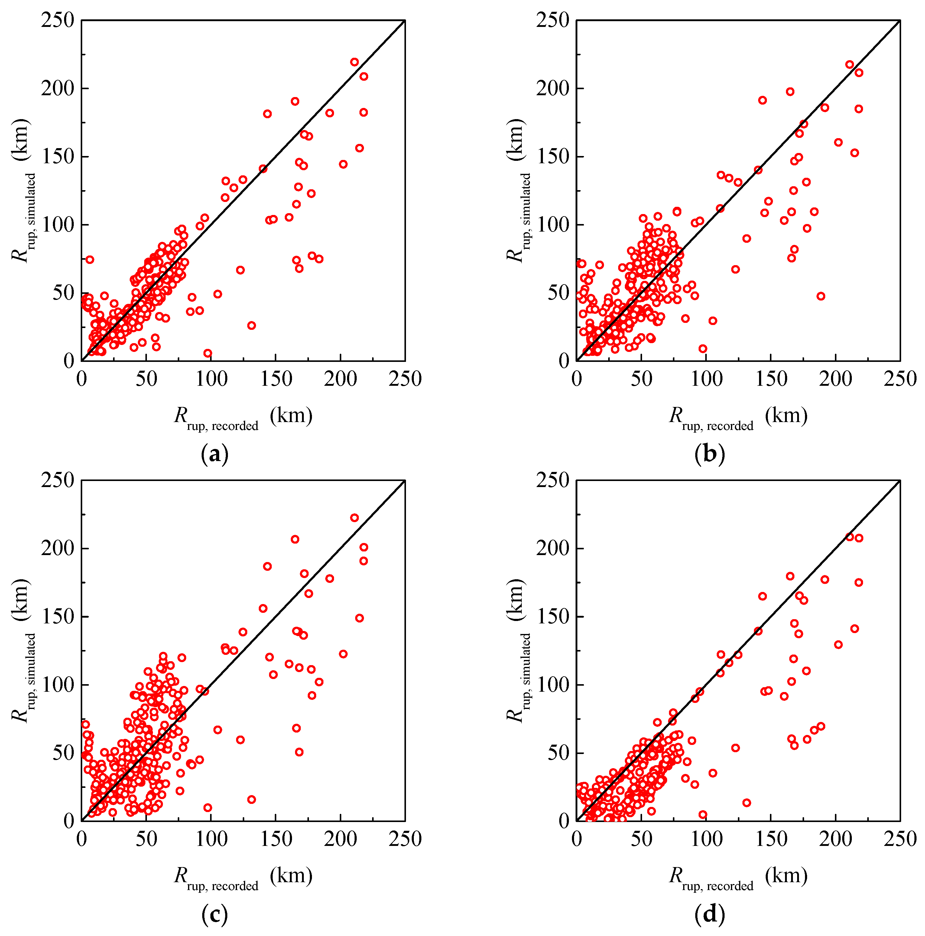
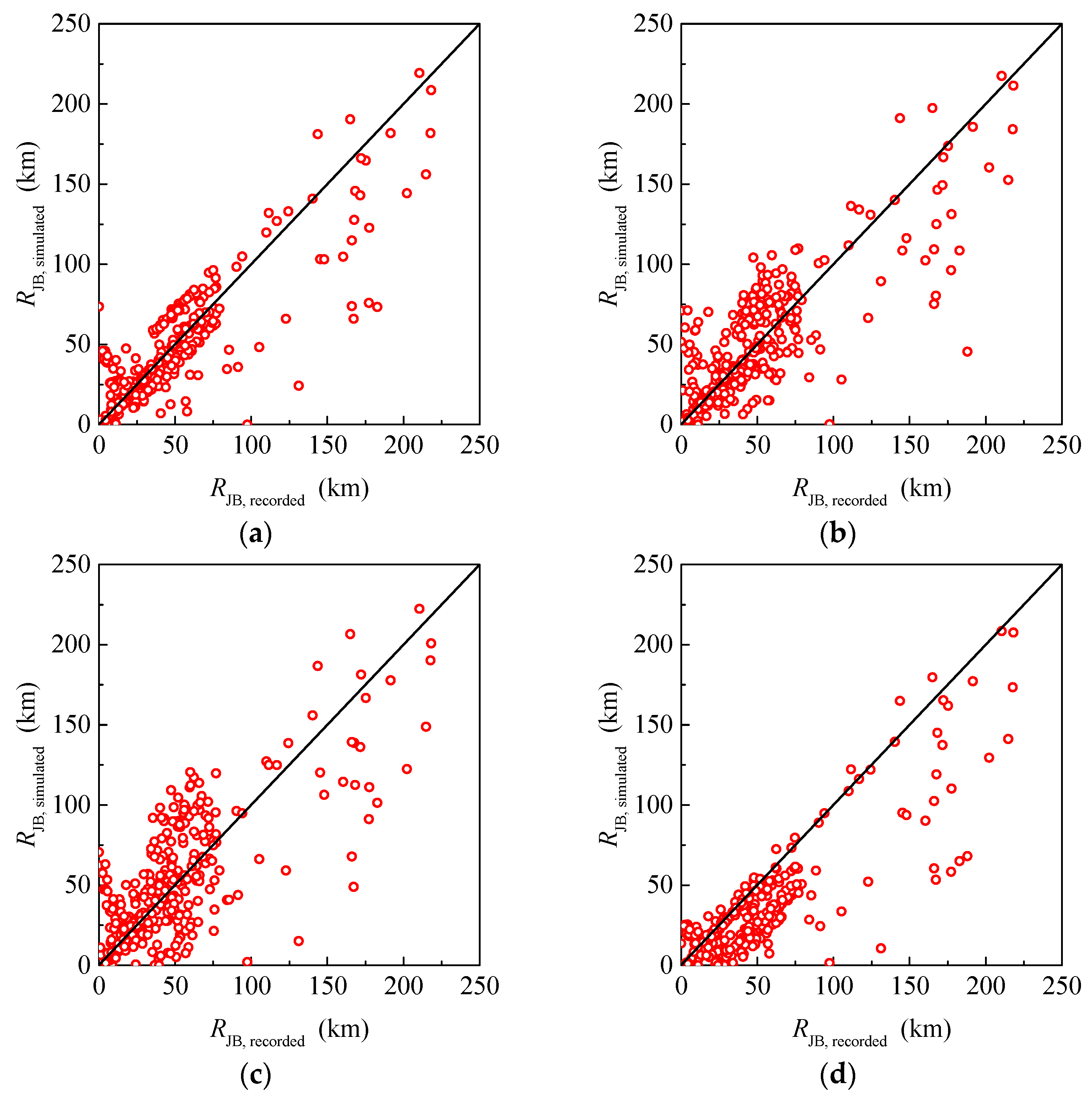
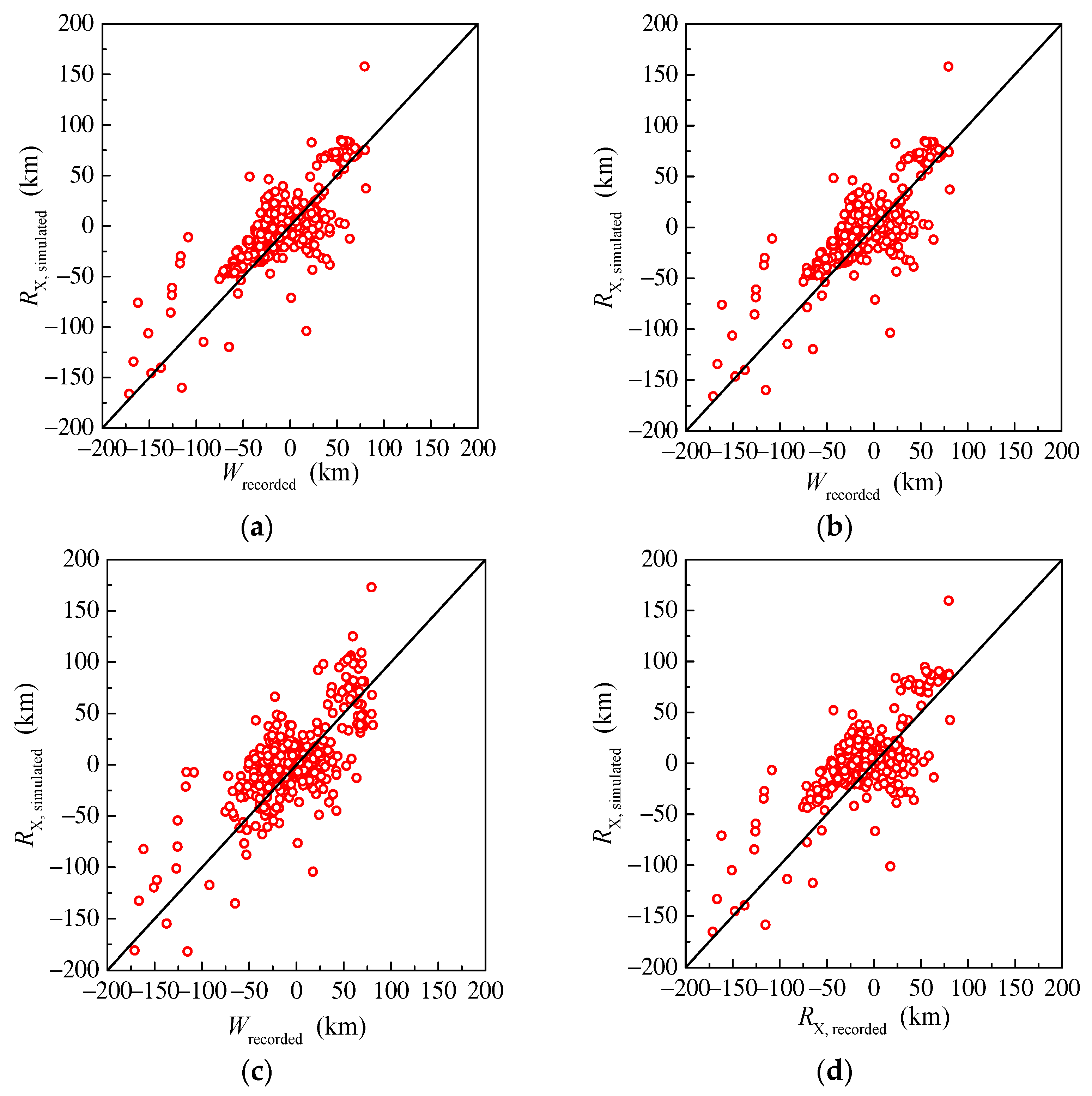
3.2. The Parameters Related to the Distance
Many parameters are related to the distance in the ASK14 model, for example, the rupture distance, the Joyner–Boore distance, etc. By determining the rupture plane of the aftershock, including the location and size, these parameters related to the distance can be determined according to their definitions.
Figure 4 shows the definition of the centroid Joyner–Boore distance (CRJB), which is the closed distance between the centroid of the Joyner–Boore rupture surface of the aftershock and the closest point on the edge of the Joyner–Boore rupture surface of the mainshock [36]. CRJB is equal to zero under the assumption that the aftershocks occur on the same place as the mainshock or that the epicenters of the aftershocks are distributed uniformly along the rupture length of the fault of the mainshock. CRJB must be determined according to its definition only in the case that the epicenters of the aftershocks are assumed to occur around the epicenter of the mainshock uniformly.
Figure 4.
Definition of CRJB [36].
Figure 5 shows the schematic diagram of the rupture distance (Rrup) and Joyner–Boore distance (RJB). As shown in Figure 2 and Figure 3, Rrup, M and RJB, M are the rupture distance and Joyner–Boore distance of the mainshock, and Rrup, A and RJB, A are the rupture distance and Joyner–Boore distance of the aftershock. RX is the distance measured perpendicular to the fault strike from the surface projection of the up-dip edge of the fault plane, as shown in Figure 6 [36].
Figure 5.
Definition of CRJB [36].
Figure 6.
Schematic diagram of RX [36].
3.3. Other Parameters
In this study, the site types of the aftershock ground motions are assumed to be the same as that of the mainshock ground motion. This means some parameters about the site model in the ASK14 model, such as the shear-wave velocity over the top 30 m (VS30), depth to VS = 1.0 km/s at the site (m) (Z1), etc., are assumed to be the same as the mainshock ground. As mentioned previously, three fault types are involved in the ASK14 model: (1) reverse, (2) normal, and (3) others. After the mainshock, determining which fault type of aftershocks is likely to happen is complicated and beyond the scope of this study. According to the research by Han et al. [37], these fault types are assumed to happen randomly and have equal probability. As for the parameters related to the hanging wall site, whether the site is within the hanging wall region is determined according to Figure 7 [36]. HW, FW, and NU mean that the site is within the hanging wall region, the footwall region, or the neutral region, respectively. Even if the site is within the hanging wall region, whether the hanging wall effect exists also relates to the fault type [38]. The hanging wall effect is assumed to exist for all fault types to simplify the procedure. If the site is located in the hanging wall region, the hanging wall effect is considered to exist.
Figure 7.
Schematic diagram of the hanging wall effect [36].
4. Conditional Mean Spectrum of the Aftershocks
The seismic parameters of the aftershock ground motions can be simulated according to the statistical relationship between the mainshock and its largest aftershock, given the mainshock ground motion.
4.1. The Aftershock Magnitude Is Known
4.1.1. The Simulated Seismic Parameters for the Aftershock Ground Motions
Given the magnitude of the aftershock, the other seismic parameters of the aftershock must be simulated using the above assumption. The above section gives three assumptions about where the aftershock occurred. Moreover, some researchers assume that the seismic parameters of the aftershock ground motions, except the magnitude, are identical to that of the corresponding mainshock ground motion. Therefore, this study uses four assumptions to determine the seismic parameters of the aftershock ground motions. The first assumption is that the aftershocks occur at the same location as their mainshock. The second and third assumptions are that the aftershocks are distributed uniformly along the rupture length of the fault of their mainshock [33] or uniformly distributed in a circular region [32]. The fourth assumption is that the seismic parameters of the aftershock ground motions are identical to those of the mainshock ground motions, except for the magnitude of the aftershocks [20]. For the second and third assumptions, the hypocenters of the aftershocks can be obtained via Latin hypercube sampling (LHS). The fault type of the aftershocks is simulated randomly. Then, the rupture lengths and widths of the rupture planes of the aftershocks are calculated according to Equations (5) and (6). The details of the rupture planes of the aftershocks are determined using the assumption that the strike angles and dip angles of the rupture planes of the aftershocks are identical to those of the mainshock. As a result, the other seismic parameters of the aftershocks, such as the rupture distance, the depth of the rupture, etc., can be determined further according to the definition of these parameters. Figure 8 shows the depths to the hypocenters of the aftershocks and their corresponding mainshocks. As shown in Figure 8, the data dots are distributed near the diagonal uniformly. Therefore, it is reasonable to assume that the depths of the hypocenters of the aftershocks and the one of their mainshocks are identical.
Figure 8.
The hypocenter depths of the selected MS–AS seismic sequences.
Figure 9 shows the down-dip rupture widths of the aftershocks with different assumptions, given the mainshocks. As shown in Figure 9, there are no essential distinctions between Figure 9a–c. The magnitudes of the aftershocks are equal to their actual values because only the magnitude and fault type are responsible for the down-dip rupture width. The only difference between them is the fault type of the aftershocks, which is simulated using the Monte Carlo method. Therefore, the subtle differences are caused by the different fault types of the aftershocks. The down-dip rupture widths of the aftershocks are assumed to be the same as that of the corresponding mainshock in Figure 9d. It can be found that the down-dip rupture width of the mainshocks is larger than those of their aftershocks, so the above assumption is not reasonable. A large magnitude usually leads to a large rupture because the magnitude of the mainshock is larger than those of its aftershocks.
Figure 9.
Down-dip rupture widths of the aftershocks with different assumptions listed as follows: (a) occurring at the same hypocenter; (b) linear assumption; (c) circular assumption; (d) identical to the mainshock.
Figure 10 shows the simulated rupture distances of the aftershocks with different assumptions. When the aftershock hypocenters are simulated using the linear model or the circular model, the results are similar, and the data points are evenly distributed around the diagonal. Figure 10a shows that simulated data points are clustered around the diagonal, but most simulated results are smaller than the real ones. As shown in Figure 10d, almost all the data points are distributed below the diagonal, which means that the simulation results are far from the real situations. The real rupture distances of the aftershocks are greater than that of the mainshock in general. Therefore, the assumption that the rupture distances of the aftershock are equal to that of the mainshock is unreasonable.
Figure 10.
Rupture distances of the aftershock ground motions with different assumptions listed as follows: (a) occurring at the same hypocenter; (b) linear assumption; (c) circular assumption; (d) identical to the mainshock.
Figure 11 shows the Joyner–Boore distances of the aftershocks simulated under different assumptions. Overall, the results are consistent with those of the rupture distances of the aftershocks. Compared with the other assumptions, the first assumption has the best result. The results of the linear model and the circular model are similar. The result of the fourth assumption is deeply unreasonable.
Figure 11.
Joyner–Boore distances of the aftershock ground motions with different assumptions, listed as follows: (a) occurring at the same hypocenter; (b) linear assumption; (c) circular assumption; (d) identical to the mainshock.
Figure 12 shows the horizontal distances from the top edges of the rupture of the aftershock ground motions simulated with different assumptions. The results of the first assumption are very similar to those of the second assumption. The values simulated according to the first and second assumptions are larger than the actual values of the aftershock ground motions in general. The data points in Figure 12c are uniformly distributed on two sides of a diagonal line, but their dispersions are relatively high. In Figure 12d, the horizontal distances from the top edges of the rupture of the aftershock ground motions are assumed to be the same as those of the mainshock ground motions. As shown in Figure 12d, the horizontal distance from the top edge of the rupture of the mainshock ground motions is larger than those of the aftershock ground motions. Therefore, the fourth assumption will introduce bias compared with the other assumptions.
Figure 12.
Horizontal distances from the top edges of the rupture of the aftershock ground motions with different assumptions listed as follows: (a) occurring at the same hypocenter; (b) linear assumption; (c) circular assumption; (d) identical to the mainshock.
4.1.2. The Response Spectrum of the Aftershock Ground Motions
With the determination of the seismic parameters of the aftershock ground motions, the median response spectrum can be predicted using the ASK14 model [31]. Then, the conditional mean spectrum of aftershocks can be computed according to Equation (1). Figure 13a shows the response spectrum predicted using the ASK14 model and the conditional mean spectrum of aftershocks with the assumption that the aftershocks and mainshock occur at the same hypocenter. Meanwhile, the recorded response spectrum of the aftershock ground motions is also shown in Figure 13a. As shown in Figure 13a, the response spectrum predicted using the ASK14 model and the conditional mean spectrum of aftershocks are lower than the recorded spectra in the short and median periods in general, but it is just the opposite in long periods. Compared with the response spectrum predicted using the ASK14 model, the conditional mean spectrum of aftershocks matches the recorded spectrum better, no matter the median or the percentiles.
Figure 13.
Conditional mean spectrum of aftershocks, with the assumption that the aftershocks and its mainshock occur at the same hypocenter and its relative errors, listed as follows: (a) conditional mean spectrum of aftershocks and (b) relative error.
The relative error (Rerror) is calculated as follows:
where is the mean of the logarithm of the predicted response spectrum, which is the response spectrum predicted using the ASK14 model or the conditional mean spectrum of aftershocks, and is the mean of the logarithm of the recorded response spectrum for the aftershock ground motions.
Figure 13b shows the relative errors of the median of the response spectrum predicted using the ASK14 model and the conditional mean spectrum of aftershocks. As shown in Figure 13b, the relative errors of the conditional mean spectrum of aftershocks are smaller than those of the response spectrum predicted using the ASK14 model in general. For the short and median periods, the relative errors of the conditional mean spectrum of aftershocks are nearly less than 10%, and range between 10% and 20% for the long periods. In contrast, the relative errors of the response spectrum predicted using the ASK14 model increase gradually, even reaching up to 70%.
Figure 14 shows the median and percentiles of the response spectrum predicted using the ASK14 model, the conditional mean spectrum of aftershocks with the linear model, showing that the epicenters of the aftershocks are uniformly distributed along the rupture length of the fault of their mainshock. The general trends with the linear model are similar to those with the assumption that the aftershock and its mainshock occur at the same hypocenter. For comparison purposes, Figure 15 shows the median and percentiles of the response spectrum predicted using the ASK14 model with the actual seismic parameters of the aftershock ground motions and the conditional mean spectrum of aftershocks. In contrast, the general trends in Figure 13 and Figure 14 are in accordance with those in Figure 15, especially the relative errors of the response spectrum predicted using the ASK14 model. Therefore, the seismic parameters of the aftershock ground motions can be reasonably simulated with the assumption that the aftershocks and mainshock occur at the same hypocenter or that the epicenters of the aftershocks are uniformly distributed along the rupture length of the fault of their mainshock.
Figure 14.
Conditional mean spectrum of aftershocks generated according to the linear model and its relative errors listed as follows: (a) conditional mean spectrum of aftershocks and (b) relative errors.
Figure 15.
Conditional mean spectrum of aftershocks generated according to the actual seismic parameters of the aftershock ground motions and their relative errors listed as follows: (a) conditional mean spectrum of aftershocks and (b) relative errors.
Figure 16 shows the median and percentiles of the response spectrum predicted using the ASK14 model and the conditional mean spectrum of aftershocks with the circular model and their relative errors. The response spectrum predicted using the ASK14 model with the circular model differs from those calculated according to the actual seismic parameters of the aftershock ground motions, especially for the median and long periods. Even so, the relative errors of the response spectrum predicted using the ASK14 are still at a low level. Meanwhile, the conditional mean spectrum of aftershocks can remain below 20% and match the recorded spectrum better than the response spectrum predicted using the ASK14 model. The only difference between the circular model and the above two assumptions is the location of the hypocenter or location of the rupture of the aftershock. Beyond that, the depth of the aftershock hypocenter, the strike and dip direction, etc., are identical to those of the first or second assumption. Therefore, the difference in the locations of the aftershock hypocenters leads to a difference in the other seismic parameters of the aftershock ground motions related to the aftershock rupture, which can lead to a difference in the response spectrum of the aftershock ground motions. For example, the simulated rupture distance and the Joyner–Boore distance with the circular model are larger than those with the first and second assumptions, as shown in Figure 10 and Figure 11. The larger rupture distance and the Joyner–Boore distance further lead to the lower response spectrum predicted using the ASK14 model. In this case, it does not mean that the circular model is unreasonable, but only that it is not suitable for the aftershock ground motions selected in this paper. The selected aftershock ground motions are only from 13 mainshock–aftershock earthquake sequences; therefore, the circular model is determined using the number of mainshock–aftershock earthquakes.
Figure 16.
Conditional mean spectrum of aftershocks generated according to the circular model and its relative errors listed as follows: (a) conditional mean spectrum of aftershocks and (b) relative error.
Figure 17 shows the response spectrum of the aftershock ground motions predicted using the ASK14 model and the conditional mean spectrum of aftershocks under the fourth assumption that the magnitude of the aftershock is equal to its actual value and the other seismic parameters are set to those for its mainshock. As shown in Figure 17, the response spectrum predicted using the ASK14 model is higher than the recorded spectrum of the aftershock ground motions for the whole period. The response spectrum has relative errors of 10% to 50% when the period is less than 3 s. After that, the relative errors become larger and larger, even reaching up to about 280%. In this case, the conditional mean spectrum of aftershocks cannot match the recorder spectrum very well.
Figure 17.
Conditional mean spectrum of aftershocks, with the assumption that the seismic parameters of the aftershocks and the mainshock ground motions are identical except the magnitude and their relative errors, listed as follows: (a) conditional mean spectrum of aftershocks and (b) relative error.
The major reason for the above results is that the seismic parameters of the aftershock ground motions are different from those of the mainshock ground motions, especially the rupture distance and Joyner–Boore distance. The rupture distance and Joyner–Boore distance of the mainshock ground motion are shorter than those of the aftershock ground motions, which leads to a larger response spectrum predicted using the ASK14 model. When calculating the response spectrum using the ASK14 model, the flag for aftershocks is set to one, and the parameter CRJB is set to zero for the aftershock ground motions.
4.2. The Aftershock Magnitude Is Unknown
This paper gives a reasonable response spectrum of the aftershock ground motion with the actual magnitude of an aftershock and other simulated seismic parameters. If the magnitude of the aftershock is unknown, the major problem becomes reasonably determining the magnitude of the aftershock. In past research, the magnitudes of the aftershocks have been widely studied. The magnitudes of the aftershocks can be supposed to have certain values for some specific research purposes. Furthermore, the magnitudes of the aftershocks could be determined via the generalized Omori’s law. Moreover, the magnitude difference between the mainshock and its largest aftershock can be determined according to some distributions. Then, the magnitude difference can be subtracted from the mainshock magnitude to obtain the magnitude of the largest aftershock.
In this paper, the magnitude difference is generated via the beta distribution, with a mean of the magnitude difference of 1.2. However, the mean of the magnitude difference is about 0.8 for the selected 662 MS–AS ground motions. In this case, it will introduce bias if the beta distribution is used to generate the magnitude difference for the selected MS–AS ground motions. Thus, this paper selects 150 MS–AS ground motions from the 662 MS–AS ground motions to ensure the magnitude difference of the reselected MS–AS ground motions is about 1.2. Table 2 shows the list of the reselected MS–AS earthquake sequences. The number of stations is set to 0.5 because the magnitudes of the Friuli and Coalinga earthquake sequences are the same, and only one station is reselected from them. Table 2 gives the number of the reselected stations for a certain MS–AS earthquake sequence. For example, 40 stations are reselected from 147 stations for the Chi-Chi earthquake, and the choice is completely random.
Table 2.
List of the reselected MS–AS earthquake sequences.
4.2.1. The Simulated Seismic Parameters for the Aftershock Ground Motions
Every mainshock ground motion is treated as an isolated earthquake, and the magnitude difference is simulated for every mainshock ground motion in the LHS. As a result, the different ground motions from the same mainshock will have a unique aftershock with a different magnitude, as shown in Figure 18. The magnitudes of the simulated aftershocks are slightly less than their actual values because the magnitude differences in the reselected MS–AS are slightly less than 1.2.
Figure 18.
The magnitudes of the aftershock ground motions utilizing LHS.
With the determination of the aftershock magnitudes, the other seismic parameters, such as the width of the rupture, the rupture distance, etc., are simulated with different assumptions about where the aftershock hypocenter will occur. Figure 19 shows the simulated rupture distances and their actual values for the reselected MS–AS ground motions. As shown in Figure 19a–c, the data dots are distributed uniformly on both sides of the 45° diagonal line. The data dots in Figure 19c are more dispersed than those in Figure 19a,b, in which the distribution of the data dots is similar. It still cannot give a reasonable result when the rupture of the aftershocks is assumed to be the same as that of the mainshock, as shown in Figure 19d. The results of the other simulated parameters are similar to those when the aftershock magnitude is known. Therefore, this paper does not provide all the details about the other simulated seismic parameters.
Figure 19.
Rupture distances of the aftershock ground motions, with different assumptions when the seismic information of the aftershock is unknown, listed as follows: (a) occurring at the same hypocenter; (b) linear assumption; (c) circular assumption; (d) identical to the mainshock.
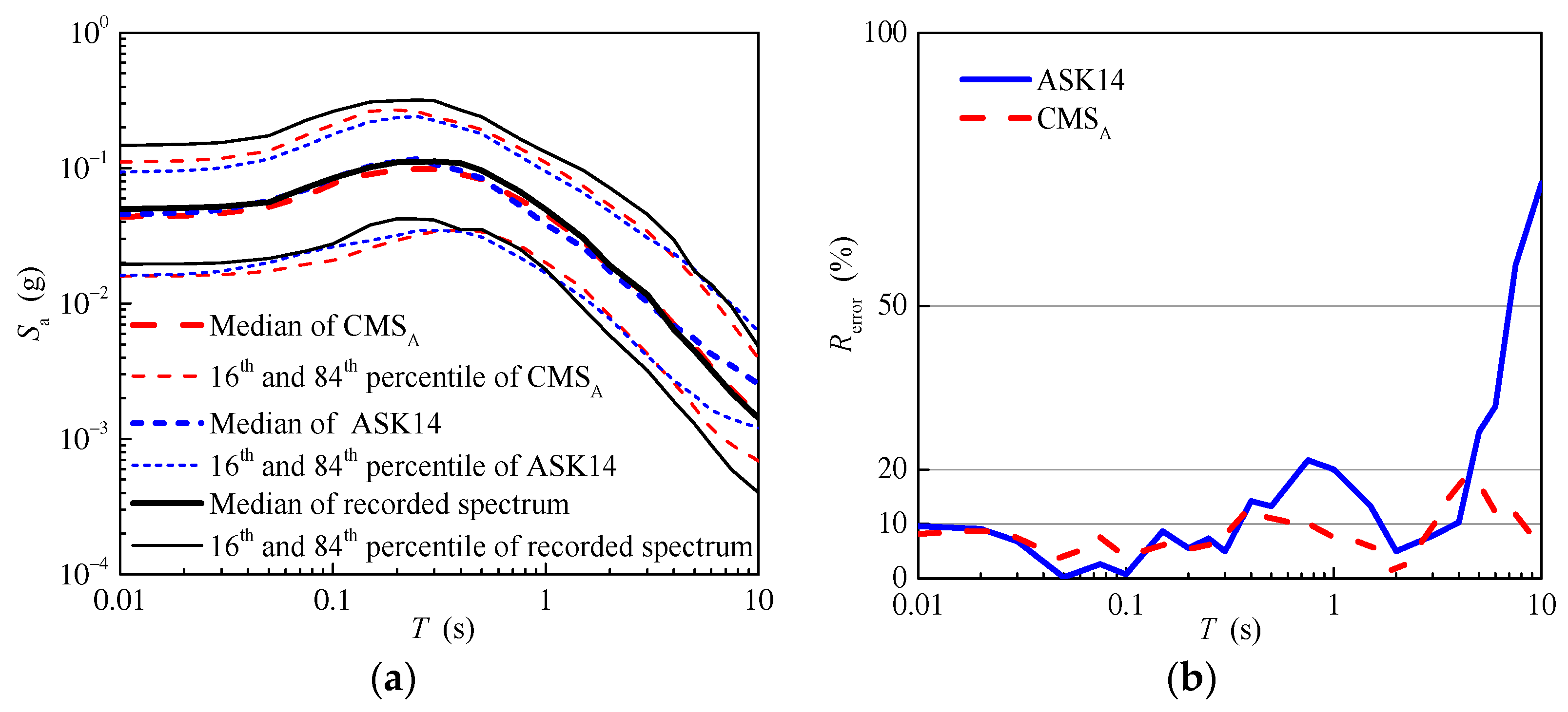
4.2.2. The Response Spectrum of the Aftershock Ground Motions
With the simulated magnitudes and different assumptions about the locations of the aftershock hypocenters, the response spectrum predicted using the ASK14 model and the conditional mean spectrum of aftershocks are calculated given the reselected mainshock ground motions, as shown in Figure 20, Figure 21, Figure 22 and Figure 23. The simulated magnitudes of the aftershock ground motions with the different assumptions come from the same sample, which are shown in Figure 18. The results show that all the assumptions, except the last one, can provide a similar response spectrum predicted using the ASK14 model. Moreover, the conditional mean spectrum of aftershocks matches the recorded spectrum better, and its relative errors are less than 20%. The best results come from the linear model under the first three assumptions. When the seismic parameters of the aftershocks are set to those of the mainshock, except the magnitude, the response spectrum predicted using the ASK14 model is very different from the recorded spectrum and has a large relative error. In this case, the conditional mean epsilon of the aftershocks cannot modify the response spectrum predicted using the ASK14 model to make the conditional mean spectrum of the aftershocks match the recorded spectrum well.
Figure 20.
Conditional mean spectrum of aftershocks, with the assumption that the aftershocks and their mainshock occur at the same hypocenter and their relative errors when the seismic information of the aftershock is unknown, listed as follows: (a) conditional mean spectrum of aftershocks and (b) relative errors.
Figure 21.
Conditional mean spectrum of aftershocks generated according to the linear model and its relative errors when the seismic information of the aftershocks is unknown listed as follows: (a) conditional mean spectrum of aftershocks and (b) relative errors.
Figure 22.
Conditional mean spectrum of aftershocks generated according to the circular model and its relative error when the seismic information of the aftershocks is unknown listed as follows: (a) conditional mean spectrum of aftershocks and (b) relative errors.
Figure 23.
Conditional mean spectrum of aftershocks, with the assumption that the seismic parameters of the aftershocks and the mainshock ground motions are identical except the magnitudes and their relative errors when the seismic information of the aftershock is unknown, listed as follows: (a) conditional mean spectrum of aftershocks and (b) relative errors.
5. Conclusions
In this paper, a new method of generating the aftershock target spectrum according to the conditional mean spectrum of aftershocks is established, given information about the main shock. The target aftershock spectrum is compared with that predicted using the ground motion prediction model, and the relative errors are also analyzed under four assumptions. The following main conclusions can be drawn.
(1) In addition to the last assumption, the relative errors of the conditional mean spectra of aftershocks are relatively small, basically controlled within the range of 20%, and its discrete properties are closer to the real recorded response spectra. This is because the correlation between the spectral shapes of the mainshock and aftershock ground motion is further considered based on the ground motion prediction equation.
(2) For the first three assumptions, the method proposed in this paper can reasonably simulate the parameters of aftershock ground motions under the given main earthquake information. Under these assumptions, the sizes of the aftershock faults can be considered, and other parameters are solved according to the definition to ensure that the simulated parameters are close to the real parameters. The parameters simulated under the first assumption are relatively concentrated, although some of its parameters, such as RJB, may be relatively larger than their real value.
In this research, a new method was developed to generate the target aftershock spectrum. The key parts are the simulation of the aftershock magnitude, the location and size of the aftershock rupture, and the correlation model of the spectral shape (epsilon) between the MS–AS ground motions. The target aftershock spectrum could be used to select aftershock ground motions from the real ground motion database or generate artificial aftershock grounds, given the mainshock ground motion.
Author Contributions
Conceptualization, D.L.; methodology, D.L.; software, R.Z. and B.D.; validation, D.L.; investigation, R.Z., B.D. and Y.Y.; writing—original draft preparation, R.Z. and B.D.; writing—review and editing, D.L. and Y.Y.; visualization, R.Z. and B.D.; supervision, D.L. All authors have read and agreed to the published version of the manuscript.
Funding
This study is founded by the Hebei Provincial Department of Human Resources and Social Security (Grant No. B2019003025).
Data Availability Statement
The selected ground motions were from the NGA-West2 ground motion database of the PEER ground motion database http://ngawest2.berkeley.edu/site (accessed on 5 October 2016).
Acknowledgments
The authors would like to gratefully acknowledge the support of the Hebei Provincial Department of Human Resources and Social Security (Personnel Department). For its work in ground motion database, the Pacific Earthquake Engineering Research Center (PEER) is also acknowledged.
Conflicts of Interest
The authors declare no conflict of interest.
List of Abbreviations and Symbols
| Abbreviations: | (Alphabetically!!) |
| AS | Aftershock |
| ASK14 | GMPE proposed by Abrahamson et al. in 2014 [31] |
| CMSA | Conditional mean spectrum of aftershocks |
| ETAS | Epidemic-type aftershock sequence |
| GMPE | Ground motion prediction equation |
| MS | Main shock |
| Probability density function | |
| Symbols: | (Alphabetically!!) |
| A | Area of the circular region (km2) |
| a, b | Regression coefficients of the rupture length and rupture width |
| Beta function for the corresponding elements 2.2 and 2.3 | |
| CRJB | Centroid Joyner–Boore distance |
| FW | Site within the footwall region |
| HW | Site within the hanging wall region |
| L | Rupture length |
| LA | Rupture length of the aftershock |
| LM | Rupture length of the main shock |
| MA | Magnitude of the aftershock |
| MM | Magnitude of the main shock |
| NU | Site within the neutral region |
| PDF of the selected beta distribution | |
| RA | Source-to-site distance of an aftershock |
| Rerror | Relative error |
| Rrup, A | Rupture distance of the aftershock |
| Rrup, M | Rupture distance of the main shock |
| RX | Distance measured perpendicular to the fault strike from the surface projection of the up-dip edge of the fault plane |
| Sa,A | Spectral accelerations of the aftershock |
| Sa,M | Spectral accelerations of the mainshock |
| Ti | The ith period of the response spectrum |
| W | Rupture width |
| WA | Rupture width of the aftershock |
| WM | Rupture width of the main shock |
| Δm | Magnitude difference between the mainshock and its largest aftershock |
| Epsilon values of the aftershock | |
| Epsilon values of the mainshock | |
| Mean of lnSa,A predicted using the GMPE | |
| Conditional mean of the lnSa,A conditioned on the lnSa,M at the period Ti | |
| Mean of the logarithm of the recorded response spectrum for the aftershock ground motions | |
| Mean of the logarithm of the predicted response spectrum | |
| at the period | |
| at the period Ti | |
| at the period | |
| Correlation coefficient between and at the period | |
| Standard deviation of lnSa,A predicted using the GMPE | |
| at the period | |
| at the period |
References
- Kam, W.Y.; Pampanin, S.; Elwood, K. Seismic performance of reinforced concrete buildings in the 22 February Christchurch (Lyttleton) earthquake. Bull. N. Z. Soc. Earthq. Eng. 2011, 44, 239–278. [Google Scholar] [CrossRef]
- Torfehnejad, M.; Sensoy, S. Aftershock collapse capacity assessment of special steel moment frame structures. Structures 2023, 56, 105046. [Google Scholar] [CrossRef]
- Saed, G.; Balomenos, G.P. Fragility framework for corroded steel moment-resisting frame buildings subjected to mainshock-aftershock sequences. Soil Dyn. Earthq. Eng. 2023, 171, 107975. [Google Scholar] [CrossRef]
- Rajabi, E.; Golestani, Y. Study of steel buildings with LCF system under critical mainshock-aftershock sequence: Evaluation of fragility curves and estimation of the response modification factor by artificial intelligence. Structures 2023, 56, 105044. [Google Scholar] [CrossRef]
- Huang, X.; Liu, J.; Wang, N.; Xu, S. Pseudo-dynamic experimental study on seismically isolated prefabricated RC structure with roller-bearing subjected to mainshock-aftershock sequences. J. Build. Eng. 2023, 65, 105775. [Google Scholar] [CrossRef]
- Tesfamariam, S.; Goda, K. Risk assessment of CLT-RC hybrid building: Consideration of earthquake types and aftershocks for Vancouver, British Columbia. Soil Dyn. Earthq. Eng. 2022, 156, 107240. [Google Scholar] [CrossRef]
- Pang, R.; Zai, D.; Xu, B.; Liu, J.; Zhao, C.; Fan, Q.; Chen, Y. Stochastic dynamic and reliability analysis of AP1000 nuclear power plants via DPIM subjected to mainshock-aftershock sequences. Reliab. Eng. Syst. Saf. 2023, 235, 109217. [Google Scholar] [CrossRef]
- Fang, C.; Ping, B.; Zheng, Y.; Ping, Y.; Ling, H. Seismic fragility and loss estimation of self-centering steel braced frames under mainshock-aftershock sequences. J. Build. Eng. 2023, 73, 106433. [Google Scholar] [CrossRef]
- Du, M.; Zhang, S.; Wang, C.; She, L.; Li, J.; Lu, T. Seismic fragility assessment of aqueduct bent structures subjected to mainshock-aftershock sequences. Eng. Struct. 2023, 292, 116505. [Google Scholar] [CrossRef]
- Pang, R.; Xu, B.; Zhou, Y.; Zhang, X.; Wang, X. Fragility analysis of high CFRDs subjected to mainshock-aftershock sequences based on plastic failure. Eng. Struct. 2020, 206, 110152. [Google Scholar] [CrossRef]
- Hatzigeorgiou, G.D.; Beskos, D.E. Inelastic displacement ratios for SDOF structures subjected to repeated earthquakes. Eng. Struct. 2009, 31, 2744–2755. [Google Scholar] [CrossRef]
- Li, Y.; Song, R.; Van De Lindt, J.W. Collapse fragility of steel structures subjected to earthquake mainshock-aftershock sequences. J. Struct. Eng. 2014, 140, 04014095. [Google Scholar] [CrossRef]
- Torres, J.R.; Bojórquez, E.; Bojórquez, J.; Leyva, H.; Ruiz, S.E.; Reyes-Salazar, A.; Palemón-Arcos, L.; Rivera, J.L.; Carvajal, J.; Reyes, H.E. Improving the seismic performance of steel frames under mainshock–aftershock using post-tensioned connections. Buildings 2023, 13, 1676. [Google Scholar] [CrossRef]
- Furinghetti, M.; Lanese, I.; Pavese, A. Experimental hybrid simulation of severe aftershocks chains on buildings equipped with curved surface slider devices. Buildings 2022, 12, 1255. [Google Scholar] [CrossRef]
- Wei, J.; Ying, H.; Yang, Y.; Zhang, W.; Yuan, H.; Zhou, J. Seismic performance of concrete-filled steel tubular composite columns with ultra high performance concrete plates. Eng. Struct. 2023, 278, 115500. [Google Scholar] [CrossRef]
- Zheng, X.; Shen, Y.; Zong, X.; Su, H.; Zhao, X. Vulnerability analysis of main aftershock sequence of aqueduct based on incremental dynamic analysis method. Buildings 2023, 13, 1490. [Google Scholar] [CrossRef]
- Ruiz-García, J.; Ramos-Cruz, J.M. Collapse strength ratios for structures under mainshock-aftershock subduction seismic sequences. Structures 2023, 56, 104864. [Google Scholar] [CrossRef]
- Nugroho, L.Z.; Chiu, C.-K. Damage-controlling seismic design of low- and mid-rise RC buildings considering mainshock-aftershock sequences. Structures 2023, 57, 105099. [Google Scholar] [CrossRef]
- Yakhchalian, M.; Yakhchalian, M. An advanced intensity measure for aftershock collapse fragility assessment of structures. Structures 2022, 44, 933–946. [Google Scholar] [CrossRef]
- Goda, K.; Taylor, C.A. Effects of aftershocks on peak ductility demand due to strong ground motion records from shallow crustal earthquakes. Earthq. Eng. Struct. Dyn. 2012, 41, 2311–2330. [Google Scholar] [CrossRef]
- Kim, B.; Shin, M. A model for estimating horizontal aftershock ground motions for active crustal regions. Soil Dyn. Earthq. Eng. 2017, 92, 165–175. [Google Scholar] [CrossRef]
- Hu, S.; Gardoni, P.; Xu, L. Stochastic procedure for the simulation of synthetic main shock-aftershock ground motion sequences. Earthq. Eng. Struct. Dyn. 2018, 47, 2275–2296. [Google Scholar] [CrossRef]
- Wang, G.; Pang, R.; Yu, X.; Xu, B. Permanent displacement reliability analysis of soil slopes subjected to mainshock-aftershock sequences. Comput. Geotech. 2023, 153, 105069. [Google Scholar] [CrossRef]
- Pu, W.; Li, Y. Evaluating structural failure probability during aftershocks based on spatiotemporal simulation of the regional earthquake sequence. Eng. Struct. 2023, 275, 115267. [Google Scholar] [CrossRef]
- Khalil, C.; Lopez-Caballero, F. Lifetime response of a liquefiable soil foundation-embankment system subjected to sequences of mainshocks and aftershocks. Soil Dyn. Earthq. Eng. 2023, 173, 108107. [Google Scholar] [CrossRef]
- Ghotbi, A.R.; Taciroglu, E. Conditioning criteria based on multiple intensity measures for selecting hazard-consistent aftershock ground motion records. Soil Dyn. Earthq. Eng. 2020, 139, 106345. [Google Scholar] [CrossRef]
- Ding, Y.; Chen, J.; Shen, J. Prediction of spectral accelerations of aftershock ground motion with deep learning method. Soil Dyn. Earthq. Eng. 2021, 150, 106951. [Google Scholar] [CrossRef]
- Chaiyasarn, K.; Buatik, A.; Mohamad, H.; Zhou, M.; Kongsilp, S.; Poovarodom, N. Integrated pixel-level CNN-FCN crack detection via photogrammetric 3D texture mapping of concrete structures. Autom. Constr. 2022, 140, 104388. [Google Scholar] [CrossRef]
- Abadel, A.A. Physical, mechanical, and microstructure characteristics of ultra-high-performance concrete containing lightweight aggregates. Materials 2023, 16, 4883. [Google Scholar] [CrossRef]
- Zhu, R.G.; Lu, D.G.; Yu, X.H.; Wang, G.Y. Conditional mean spectrum of aftershocks. Bull. Seismol. Soc. Am. 2017, 107, 1940–1953. [Google Scholar] [CrossRef]
- Abrahamson, N.A.; Silva, W.J.; Kamai, R. Summary of the ASK14 ground motion relation for active crustal regions. Earthq. Spectra 2014, 30, 1025–1055. [Google Scholar] [CrossRef]
- Han, R.; Li, Y.; van de Lindt, J. Assessment of seismic performance of buildings with incorporation of aftershocks. J. Perform. Constr. Facil. 2015, 29, 04014088. [Google Scholar] [CrossRef]
- Yeo, G.L.; Cornell, C.A.A. probabilistic framework for quantification of aftershock ground-motion hazard in California: Methodology and parametric study. Earthq. Eng. Struct. Dyn. 2009, 38, 45–60. [Google Scholar] [CrossRef]
- Kumitani, S.; Takada, T. Probabilistic assessment of buildings damage considering aftershocks of earthquakes. J. Struct. Constr. Eng. 2009, 74, 459–465. [Google Scholar] [CrossRef]
- Wells, D.L.; Coppersmith, K.J. New empirical relationships among magnitude, rupture length, rupture width, rupture area, and surface displacement. Bull. Seismol. Soc. Am. 1994, 84, 974–1002. [Google Scholar]
- Ancheta, T.D.; Darragh, R.B.; Stewart, J.P.; Seyhan, E.; Silva, W.J.; Chiou, B.S.-J.; Wooddell, K.E.; Graves, R.W.; Kottke, A.R.; Boore, D.M. NGA-West2 database. Earthq. Spectra 2014, 30, 989–1005. [Google Scholar] [CrossRef]
- Han, R.; Li, Y.; van de Lindt, J. Seismic risk of base isolated non-ductile reinforced concrete buildings considering uncertainties and mainshock–aftershock sequences. Struct. Saf. 2014, 50, 39–56. [Google Scholar] [CrossRef]
- Abrahamson, N.; Silva, W.J. Empirical response spectral attenuation relations for shallow crustal earthquakes. Seismol. Res. Lett. 1997, 68, 94–127. [Google Scholar] [CrossRef]
Disclaimer/Publisher’s Note: The statements, opinions and data contained in all publications are solely those of the individual author(s) and contributor(s) and not of MDPI and/or the editor(s). MDPI and/or the editor(s) disclaim responsibility for any injury to people or property resulting from any ideas, methods, instructions or products referred to in the content. |
© 2023 by the authors. Licensee MDPI, Basel, Switzerland. This article is an open access article distributed under the terms and conditions of the Creative Commons Attribution (CC BY) license (https://creativecommons.org/licenses/by/4.0/).