Thermal Hysteresis Effect and Its Compensation on Electro-Mechanical Impedance Monitoring of Concrete Structure Embedded with Piezoelectric Sensor

Abstract

Piezoelectric (PZT) sensors employed in the electro-mechanical impedance/admittance (EMI/EMA) technique are vulnerable to temperature variations when applied to concrete structural health monitoring (SHM). However, in practice, the ambient temperature transmitted from the air or surface to the concrete inner part is time-dependent during its monitoring process, which inflicts a critical challenge to ensure accurate signal processing for PZT sensors embedded inside the concrete. This paper numerically and experimentally investigated the thermal hysteresis effect on EMA-based concrete structure monitoring via an embedded PZT sensor. In the numerical modeling, a 3D finite element model of a concrete cube embedded with a PZT sensor was generated, where thermal hysteresis in the concrete, adhesive coat, and sensor was fully incorporated by introducing a temperature gradient. In the experiment, an equal-sized concrete cube installed with a cement-embedded PZT (CEP) sensor was cast and heated for 180 min at four temperature regimes for EMA monitoring. Experimental results, as a cogent validation of the simulation, indicated that EMA characteristics were functionally correlated to the dual effect of both heat transfer and the temperature regime. Moreover, a new approach relying on the frequency/magnitude of the maximum resonance peak in the EMA spectrum was proposed to effectively compensate for the thermal hysteresis effect, which could be regarded as a promising alternative for future applications.

1. Introduction

Continuous on-line monitoring of concrete structures, including their external loading, operational environment, and static/dynamic responses, holds the key to understanding the origination, formation, and progression of structural anomalies, damage, and incidents, which is critically significant for the prevention of catastrophic failures in a structure or its elements. Among the numerous monitoring approaches such as acoustic emission or piezoresistive sensors by conductive materials [1,2,3,4], the piezoelectric lead zirconate titanate (PZT)-based electro-mechanical impedance/admittance (EMI/EMA, inverse of impedance) technique has been sustainably attracting intensive interest in the field of concrete structural health monitoring (SHM), involved with the monitoring of load-induced crack damages, hydration evolution, and structural tension/compression stress development [5,6,7,8]. In the EMI technique, a PZT patch can simultaneously serve as the sensor and actuator, relying on its instantaneous direct and inverse piezoelectric effects. When the PZT transducer is attached to or embedded in a host structure via an adhesive layer/coat, its electrical signal coupled to structural information, namely mechanical impedance, could be measured as the EMA spectrum. Any damage that occurs in the vicinity of the transducer can be captured and reflected by the EMA variations. However, the application of the EMI technique for monitoring in situ engineering structures is rather complicated, due to the environmental uncertainties (such as changes in temperature, humidity, and natural hazards). In particular, environmental temperature fluctuation is regarded as an adverse factor, because the PZT transducer, bonding layer, and structure are all affected by temperature changes [9,10]. The variations in EMA responses due to temperature fluctuations are significant, even surpassing the changes induced by regular structural damages [10]. Moreover, temperature fluctuations exhibit time-dependent behavior in practical scenarios, and as a result, it remains necessary to investigate the impact of the thermal hysteresis effect on the counterparts of the electro-mechanical coupled system. It could result in inaccurate alarms for damage diagnosis during the long-term SHM process if such associated effects and mechanisms remain inadequately understood.

In order to gain a better comprehension of temperature influences on the EMA-based non-destructive testing technique, many researchers have performed intensive investigations, including theoretical analyses, finite element (FE) simulations, and experimental tests. Analytical discussions about the temperature dependency of the piezoceramic sensor and its impedance characteristics showed that the shifting of resonance frequencies and fluctuations in peak response magnitude, caused by an increase in temperature, could lead to wrong conclusions regarding the damages of structures, such as steel beams, bolted pipes, and composite reinforced aluminum plates [11,12]. A few models regarding an aluminum cantilever beam [13] and a fully clamped plate [14] with attached piezoelectric wafer active sensors (PWAS) have been proposed to reveal structural responses with consideration of the temperature effect. In these models, temperature action was introduced by considering the temperature dependency of both the structure and PWAS material property, which were assumed to be uniform in each temperature condition for simplicity. In addition to an analytical investigation, the temperature effect and corresponding measurements on new piezoceramic devices such as low-cost piezoelectric diaphragms [15], bulk ceramics, and piezoceramic composite [16], which interacted with aluminum structures, were respectively presented. It was found that gradual shifts in the prominent resonance for the bonded PZT patch on an aluminum beam specimen moved to the left against the progressive elevating temperature [17]. Similar experiments conducted on an aluminum beam [18] and carbon fiber-reinforced polymer panels [19] under a given temperature also indicated that the three major characteristics, i.e., the real part, the imaginary part, and the magnitude of the impedance signatures, exhibited the approximate resonance peaks and frequency shifts. Furthermore, FE modeling was also carried out as a complementary investigation, profiting from its easier implementation for some unattainable operations, such as taking thermal responses into consideration for an additional combination of the bonding layer. Modeling on aluminum beams bonded with the PZT patch demonstrated that the admittance signatures acquired from patches with a thicker bonding layer exhibited more severe deviations than those with a thinner one, even if subjected to the same temperature [20,21].

Intending to minimize the temperature impact and discriminate it from structural damages, researchers have also developed a series of methods. For example, decoupling of the impedance for the evaluation of the temperature effect indicated that the active conductance signature had high sensitivity to structural damages and was robust to temperature fluctuations [22]. A model aimed at predicting the piezoelectric susceptance slope at any temperature to separate temperature-induced variations from those caused by sensor defects in the impedance-based SHM was also validated via an aluminum frame structure [23]. A technique integrating a sensor array and statistical metric analysis was proposed to distinguish impedance signal changes derived from damage and/or temperature disturbance [24], and principles of statistical process control, along with confidence intervals, were employed to detect saw cuts on aluminum panels within a temperature range, ensuring a 95% confidence interval [25]. Other approaches such as using matric, namely the squared sum of the real impedance variation [11], artificial neural networks [26], and the effective frequency shift method were proposed and cogently verified by experiments on bolted flange-pipe joint, steel plate, steel truss, and PSC girder structures [27,28]. Recently, a polynomial interpolation-based method has been also investigated to compensate for the temperature effect on impedance measurements in SHM [29]. These approaches aimed at reducing the variations involved with vertical and horizontal shifts in admittance/impedance signatures due to temperature deformation, thus contributing to avoiding the false detection of damages. Meanwhile, the compensation effectiveness closely relies on a comprehensive assessment of temperature influences including the thermal hysteresis effect, which is, however, not involved in previous research.

Generally, the above investigations, mainly concentrating on the coupling responses between the PZT transducer and metal structures, deemed that temperature is constant and uniform in a short time for the tested specimens under normal temperature conditions. With regard to that under extreme high-temperature conditions, the heating time is considered for oven exposure. For example, high-temperature PWAS and its attached Ti disk were subjected to oven testing for 30 min near 90 °C steps until 705 °C [30]. Only 10 min was needed for temperature stabilization as it increased from room temperature up to 200 °C per 50 °C [31]. Circular PWAS transducers were heated from 50 °C to 250 °C in 50 °C increments at a rate of 1–2 °C min⁻¹ [32]. Sometimes, an ambient temperature was directly adopted for analyzing temperature influence, such as for a thin plate of carbon fiber-reinforced polymers bonded with a piezoelectric transducer [33]. It is reasonable for the mentioned homogeneous metal or thin composite structures to reach thermal equilibrium in a short time, especially for surface-mounted PZT patches directly subjected to thermal etching. However, few studies have focused on the temperature effect on non-homogeneous concrete structures. Different from metal structures with their good thermal conductivity, concrete materials are non-homogeneous, porous, and have low thermal conductivity [34]. Therefore, they need more time to realize the balance of heat distribution. An experiment on a mortar specimen with a PZT sensor inside showed temperature dependence of the electric impedance spectra; however, the specimen put in an oven for 1 h was regarded as stable at each temperature regime ranging from −20 °C to 40 °C with a heating rate of 2 °C/min [35]. In the previous study by the first author and his colleagues [36], a quantification investigation of the temperature influence on EMA-based concrete structural damage detection was performed through theoretical, numerical, and experimental analysis, where healthy/damaged concrete specimens heated in an oven for 1 h were employed for EMA measurements of bonded and embedded PZT sensors. However, the temperature influence on concrete structural monitoring in the above studies was assumed to be stable under a given time. To comprehensively assess the impact of heating time, the primary author recently imposed surfaced-bonded PZT sensors on a concrete structure and implemented a heating procedure as long as 180 min. The outcomes indicated a strong correlation between the heating time and the temperature-induced effects on EMA spectra [37]. The difference was that surface-bonded PZT sensors are less affected by the thermal hysteresis of the inner part of concrete, while the embedded ones are constrained by the surrounding concrete being invertible from such a hysteresis effect. Unfortunately, time-varying thermal hysteresis effects on the EMA spectrum of the embedded PZT transducer inside the concrete structure have remained unresolved until now.

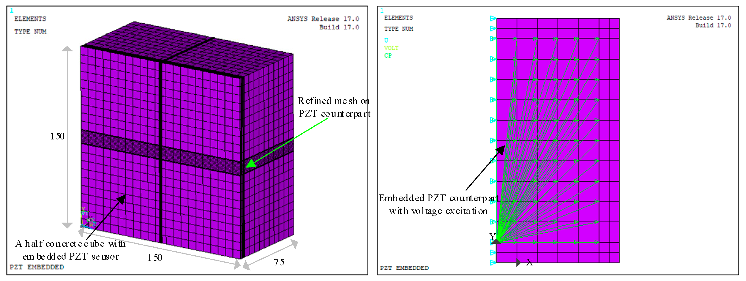
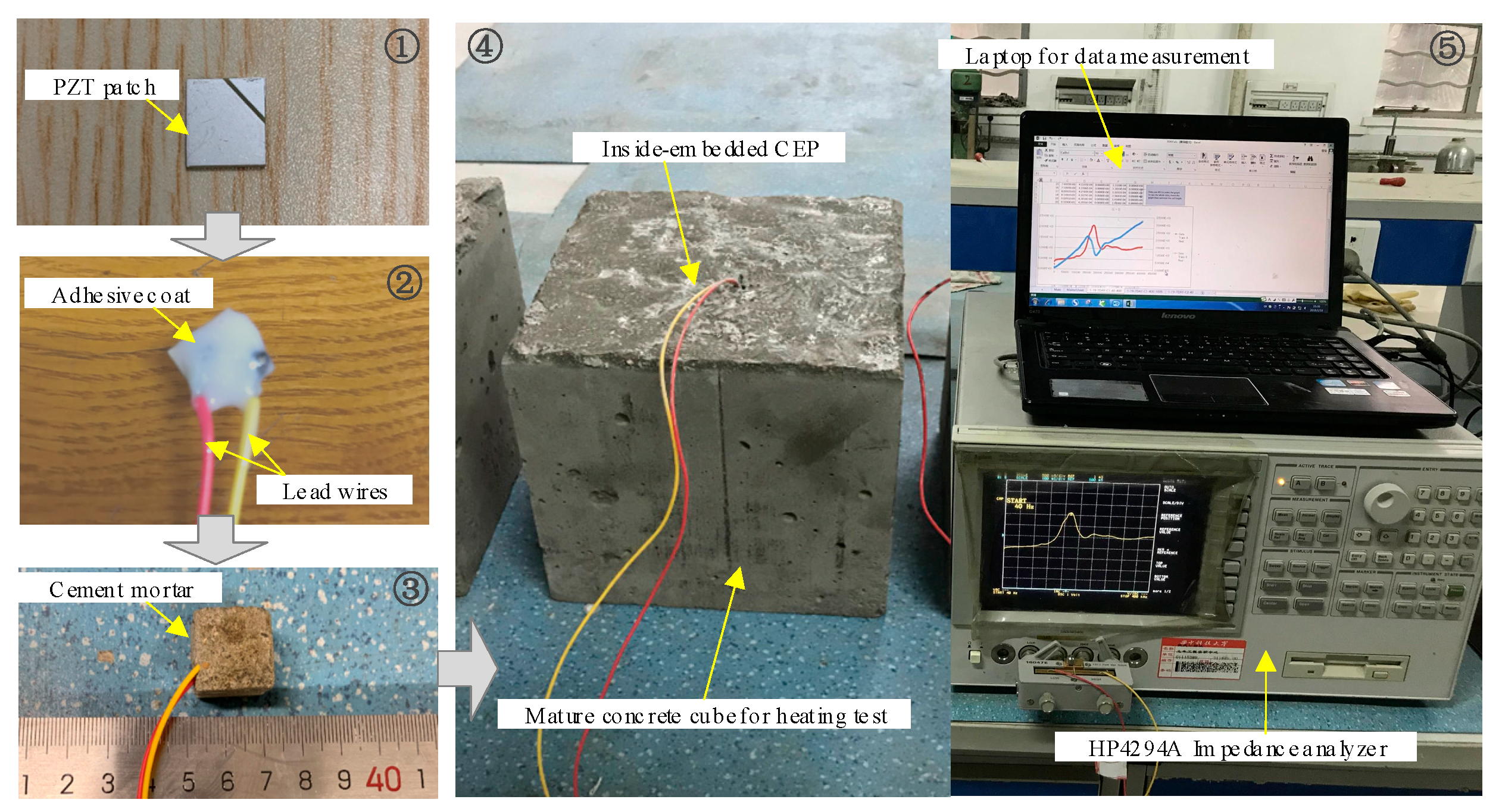
This paper, as a continuation of the previous paper [37], investigated the thermal hysteresis effect on the EMA monitoring of an embedded PZT sensor in a concrete structure using numerical modeling and experimental tests. In the numerical modeling, a 3D FE model for a concrete cube installed with a cement-embedded PZT (CEP) sensor was first generated in ANSYS version 17.0. Thermal hysteresis effect modeling was achieved by full consideration of the temperature gradient on the concrete, the PZT sensor, and its coating layer with incremental temperatures from 30 °C to 60 °C. In the experiment, a concrete cube was cast to undergo a thermal test at four distinct temperatures: 30 °C, 45 °C, 60 °C, and 75 °C, respectively. Under each condition, the cube was consistently heated for 180 min in an oven, with EMA measurements monitored every 10 min. Features of the EMA spectra and statistical indices called the baseline unvaried/varied root mean square deviation (RMSD/RMSDk) were mathematically correlated to thermal transmission. The major contributions of this article could be specified as:

(1)

The thermal hysteresis effect in thermal transmission was first investigated via the EMA monitoring of the embedded PZT transducer inside the concrete structure.

(2)

A new methodology for compensation of the thermal hysteresis effect on the EMA spectrum was proposed using the frequency and magnitude values of the maximum resonance peak.

The rest of this article is organized into four parts. Section 2 gives a brief introduction to the principle of the embedded PZT model in the EMI technique, while numerical analysis and experimental investigations on the thermal hysteresis effect on the EMA spectra and its compensation are introduced in Section 3 and Section 4, respectively. Finally, concluding remarks are made in Section 5.

2. Embedded PZT Model in EMI Technique

There are commonly two categories of PZT sensors that interact with a target structure in the EMI technique, namely surface-bonded and inside-embedded. For the surface-bonded one, Liang et al. [38] proposed a one-dimensional impedance model to reveal the energy transfer and consumption of a PZT-driven active system, where the target structure is assumed as a one-degree-of-freedom spring-mass-damper system. When imposing a voltage excitation in the thickness direction (‘3’) of the patch with a size of l × b × h, extensional strain is consequently produced, motivating structural responses as mechanical strain, as shown in Figure 1. Such strain is conversely transferred to the patch to generate an electrical signal called the EMA spectrum. In this way, any damages affected by structural impedance could be directly identified by EMA variations. For the 1D model of a surface-bonded patch, only vibration in the length (‘1’) direction is considered, and the vibrations along the width (‘2’) and thickness (‘3’) directions can be ignored.

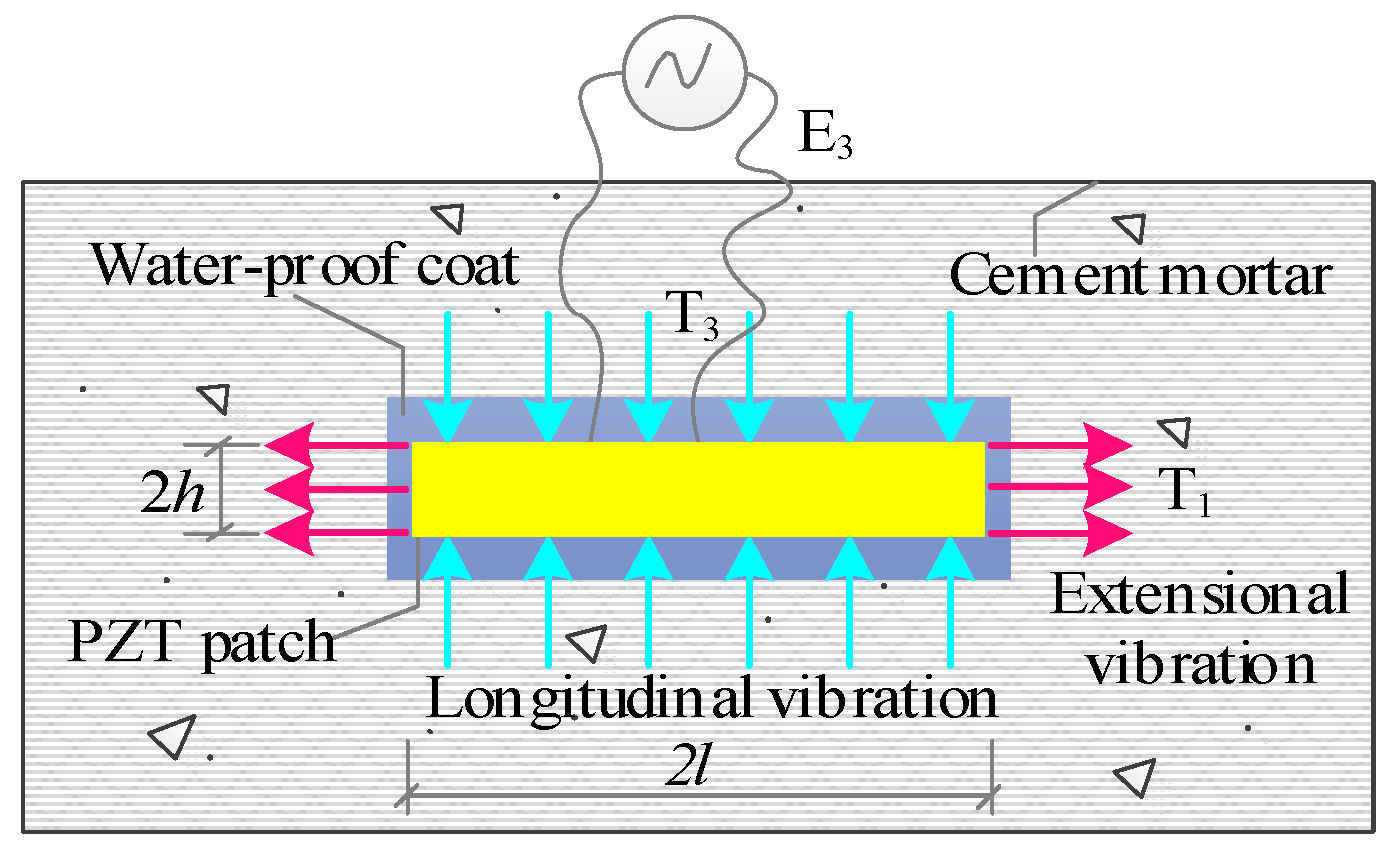
However, concerning an embedded PZT transducer, the dynamic interactions between the patch and the structure are significantly influenced by its longitudinal vibration in the ‘3’ direction, as noted in [39]. Since it is closer to reality when considering both the extensional and longitudinal vibrations in ‘1’ and ‘3’ directions for the embedded transducer, a two-dimensional model of the PZT–adhesive coat–structural interaction has been developed [40], as shown in Figure 2. The coupling of the electrical parameters (electrical field: E₃; electrical displacement: D₃) and the mechanical parameters (mechanical strain: S₁, S₃; mechanical stress: T₁, T₃) can be expressed as:

$$D_3=\overline{{\epsilon }_{33}^T}{E}_3+d_{31}{T}_1+d_{33}{T}_3,$$

(1)

$$S_1=\frac{T_1-{\nu }_{13}{T}_3}{\overline{Y^E}}+d_{31}{E}_3,$$

(2)

$$S_3=\frac{-{\nu }_{13}{T}_1+{\nu }_{33}{T}_3}{\overline{Y^E}}+d_{33}{E}_3,$$

(3)

where $\overline{{\epsilon }_{33}^T}={\epsilon }_{33}^T\left(1-j\delta \right)$ is the electric permittivity at constant stress; $\overline{Y^E}=Y^E\left(1+j\eta \right)$ is the complex Young’s modulus at constant electric field; $\delta$ denotes the dielectric loss factor; $\eta$ is the mechanical loss factor; ${\nu }_{13}$, ${\nu }_{33}$ are Poisson’s ratios; d₃₁, d₃₃ are the piezoelectric strain constants. With the aid of the definition for effective mechanical impedance, the EMA formula of the embedded PZT model shown in Figure 2 can be derived as [40]:

$$Y\left(\omega \right)=\frac{4bl\omega j}{h}\left[\overline{{\epsilon }_{33}^T}-\frac{\overline{Y^E}\left(d_{31}+n{d}_{33}\right)d_{31}}{1-n{\nu }_{13}}+\frac{\overline{Y^E}\left(d_{31}+n{d}_{33}\right)d_{31}{Z}_{a,eff}}{\left(1-n{\nu }_{13}\right)\left(Z_{a,eff}+Z_{s,eff}\right)}\left(\frac{\mathit{tan}\kappa l}{\kappa l}\right)\right],$$

(4)

where b, l, and h are the width, length, and thickness of the PZT patch, respectively; $Z_{a,eff}$ and $Z_{s,eff}$ are the effective impedance of the PZT transducer and structure, respectively; $\kappa$ denotes the wave number related to the angular frequency $\omega$; $\rho$ is the density of the patch. n denotes the value of the mechanical coupling coefficient.

In Equation (4), it is clear that the EMA value at any frequency point is closely associated with both the piezoelectric parameters and structural properties including mass, stiffness, and damping. In addition to structural damages, other parameters such as the piezoelectric strain constant and electric permittivity could also alter the EMA values, when they vary with temperature change [11]. Consequently, the EMA formula can be deemed as a function related to the temperature variable. In order to quantify the EMA variations caused by temperature, root mean square deviation (RMSD) is deemed as one of the most effective indices in the EMI technique [10], which is expressed as:

$$RMSD=\sqrt{\frac{{{\displaystyle \sum }}_{i=1}^N{(Y_i^k-Y_i^0)}^2}{{{\displaystyle \sum }}_{i=1}^N{(Y_i^0)}^2}},$$

(5)

where $Y_i^0$ and $Y_i^k$ are the pristine and corresponding EMA values of the PZT at the ith sample point for each kth case. Different from RMSD for assessing the accumulated variation compared to the healthy state, a baseline-varied index, namely RMSDk, is also improved to differentiate and evaluate the absolute variations of each condition, which is expressed as [40]:

$$RMSDk\left(\%\right)=\sqrt{\frac{{{\displaystyle \sum }}_{i=1}^N{(Y_i^k-Y_i^{k-1})}^2}{{{\displaystyle \sum }}_{i=1}^N{(Y_i^{k-1})}^2}}\times 100, k=1,2\dots n,$$

(6)

where $Y_i^{k-1}$ is the EMA spectrum at the ith sample point and considered the baseline at the prior state. The general and absolute variations in the EMA spectra throughout the heating process could be effectively evaluated by utilizing these indices. The next section covers the numerical analysis of the thermal hysteresis effect.

3. Numerical Analysis of Thermal Hysteresis Effect on EMA Spectrum of Concrete Cube Embedded with PZT Sensor

3.1. FE Model of Concrete Cube Installed with Embedded PZT Sensor

3.1.1. Multi-Field Harmonic Analysis for Piezoelectric and Structural Coupling Interaction

By way of Galerkin FE discretization, the linear electro-mechanical constitutive equations were integrated into a general equation of motion for a forced structural system, and the discretization for piezoelectric analysis could be performed [20]. As is known, the finite element method is an effective way to simulate the mechanical, electric, and polarization behaviors of piezoelectric materials under static bending and dynamic vibration [41,42,43,44]. In this study, piezoelectric analysis was conducted to simulate the mechanical and electric behaviors in commercially available FE software ANSYS version 17.0. The EMA of the PZT transducer can be determined through a multi-field harmonic analysis. Employing the FE discretization and the structural variational equation, as interpreted in [45], the coupled FE matrix for a single-element model in electric-mechanical coupling analysis can be indicated as:

$$\begin{gathered} \left[\begin{array}{cc}\left[M\right]& \left[0\right]\\ \left[0\right]& \left[0\right]\end{array}\right]\left\{\begin{array}{c}\left\{\ddot{u}\right\}\\ \left\{\ddot{v}\right\}\end{array}\right\}+\left[\begin{array}{cc}\left[C\right]\hfill & \left[0\right]\\ \left[0\right]\hfill & -\left[C^{vh}\right]\end{array}\right]\left\{\begin{array}{c}\left\{\dot{u}\right\}\\ \left\{\dot{v}\right\}\end{array}\right\}+\left[\begin{array}{cc}\left[K\right]& \left[K^Z\right]\\ {[K^Z]}^T& -\left[K^d\right]\end{array}\right]\left\{\begin{array}{c}\left\{u\right\}\\ \left\{v\right\}\end{array}\right\}= \\ \left\{\begin{array}{c}\left\{F\right\}\\ \left\{L+L^{th}\right\}\end{array}\right\}, \end{gathered}$$

(7)

where $\left[M\right]$, $\left[C\right]$, and $\left[K\right]$ signify the structural mass matrix, damping matrix, and stiffness matrix, respectively; {u} and {v} signify the vectors of nodal displacement and electric potential, respectively; $\left[K^Z\right]$ is the piezoelectric coupling matrix and $\left[K^d\right]$ is the unit dielectric conductivity matrix; {L} and $\left\{L^{th}\right\}$ are the vectors of nodal and surface/body charges induced by thermal variation, respectively; $\left[C^{vh}\right]$ is the unit dielectric damping matrix. The force vector {F} $=\left\{F^{nd}\right\}+\left\{F^{th}\right\}+\left\{F^{pr}\right\}$ including the nodal force, thermal force, and pressure. In piezoelectric analysis, the electrical charge Q(t) is the electrical reaction responding to an applied voltage. The current I(t) derived from the charge accumulated on the PZT surface electrodes can be expressed as a function of the radial frequency ω and Q(t):

$$I\left(t\right)=j\omega Q\left(t\right),$$

(8)

where $\omega =2\pi f$, f signifies the selected frequency. With the aid of Equation (8), the complex EMA formula Y(ω) could be defined as the output current I divided by the applied voltage V, which is expressed as:

$$Y\left(\omega \right)=\frac{I\left(t\right)}{V}=j\frac{2\pi fQ\left(t\right)}{V},$$

(9)

3.1.2. Embedded PZT in Concrete Structural Modeling and Validation

Firstly, a free-vibrated PZT (FVP) model was generated for piezoelectric parameter calibration, as shown in Figure 3a. The FVP patch with the size of 10 × 10 × 0.5 mm³ was modeled and simulated in ANSYS version 17.0 by utilizing the SOLID5 element, which has eight nodes with up to six DOF at each node. Material properties of the patch in the simulations are tabulated in

Table 1. Properties of PZT material in simulations.

Parameters	Values
Density $\rho$ (kg m−3)	7800
Poisson’s ratio ν	0.38
Dielectric loss factor $\tan \delta$	0.02
Damping ratio ξr	0.008
Piezoelectric strain coefficients (10−10 m V−1)	−2.1/−2.1/5.0/5.8/5.8
Compliance $S_{11}/S_{12}/S_{13}/S_{22}/S_{23}/S_{44}/S_{66}$ (10−12 m2 N−1)	15/−4.5/−5.7/19/−5.7/39/49.4
Electric permittivity ${\epsilon }_{11}^T/{\epsilon }_{22}^T/{\epsilon }_{33}^T$ (10−8 F m−1)	1.75/1.75/2.12

. The meshing size for the numerical model was determined as 0.25 mm by means of simulation experience and trial-and-error tests. Experimental validation of the FVP model has been made in the previous study by the first author [46], as shown in Figure 3b. It can be found that the resonance magnitudes of the numerical and experimental results are compatible with the proximity in a frequency range as wide as 0–1000 kHz, and multiple-peak characteristics at the major resonances of the measurement are well reflected in the modeling spectrum. Much higher resonance peaks are observed in the simulation, which is similar to previous studies [20,21], due to the manufacturing deviation and vibrational constraints caused by soldering the patch to lead wires in tests. More peaks in the experimental spectra could also be induced by the welding electrode made of Sn-Pb alloy with mass addition to the patch, while it is ideally simplified by the completely free-free condition in the simulation.

We then conduct the simulation for creating a 3D model of a concrete cube embedded with PZT, as a preparation for heating analysis. The properties of the patch are exactly the same as the model in Figure 3. The boundary condition of the cube model was simply supported according to the latter experiment. By means of the symmetrical feature of geometrical shapes, only half of the cube model was developed in ANSYS version 17.0, and accordingly, the patch set in the center of the cube was half-modeled, as shown in Figure 4. At this point, the interfacial nodes along the z-plane were constrained in the z-direction. The sizes of the concrete cube are 75 × 150 × 150 mm³, and that of the adhesive layer are 0.5 mm at each side of the PZT thickness direction and 0.5 mm at the top and bottom sides of the PZT length and width directions, respectively. Both the cube and adhesive were simulated via the SOLID45 element, with each node consisting of three DOFs. The material properties are tabulated in

Table 2. Properties of the simulated concrete and adhesive materials.

Parameters (Unit)	Symbol	Concrete	Adhesive
Density (kg/m3)	ρ	2500	1180
Young’s modulus (Pa)	E	2.80$\times$1010	4.89$\times$109
Poisson’s ratio	υ	0.26	0.38
Thermal expansivity (1/°C)	γ	6$\times$10−6	100$\times$10−6

. The meshing size was determined according to the literature [20], thus counterparts of adhesive and concrete solids were manually set as 0.5 mm, while an element size of 2 mm was adopted for the other solids, where a fitting size could improve the computation efficiency. In this study, an identical damping ratio in the harmonic analysis was conducted, i.e., 0.8%, as a robust validation for plain concrete modeling based on our prior study [36].

After the generation of the cube model, it is verified via experimental measurement before implementing it to investigate the thermal hysteresis effect. Here, the range of 30 °C to 60 °C was considered in the modeling based on the following considerations: (1) This temperature range is intended to be the same as that conducted in the latter experimental thermal test; (2) determination of such a range is expected to ensure the accuracy of the simulation as some thermal-related parameters of piezoelectric materials are approximately linear or have a certain relationship with temperature changes. There may be uncertain relationships when the temperature is higher than 60 °C. (3) In the context of concrete SHM in most areas, environmental temperatures are hardly higher than 60 °C and most are around 20 °C most of the time, which could be deemed as a reference and, accordingly, one only needs to compensate for the EMI-based SHM when it is higher than 30 °C but lower than 60 °C. Figure 5 compares the numerical and experimental conductance spectra within a frequency band of 0–400 kHz. Experimental measurement is obtained from the same concrete specimen used for the thermal test in the next section. It can be seen that the magnitudes and frequencies in the resonance of the experimental signature are well predicted by the simulation near 160 kHz and 300 kHz, and few such resonant peaks are due to the weak interaction between the transducer and the passive concrete structure [7]. It is also found that the simulated magnitude of the first resonance is much higher than the measured one, which is similar to the previous investigation [47]. The major reason for such deviation is the challenge of accurately determining the damping ratio value [46]; meanwhile, inhomogeneity in concrete materials simplified as homogeneous in the simulation can also cause errors. Moreover, a few peaks are not predicted by the simulation, which is mainly attributed to local material differences that may exist in the real concrete cube, which results in different peak characteristics of the EMA spectra [20]. Additionally, Figure 5b compares the conductance spectra of the cube under a temperature of 60 °C considering an adhesive thickness of 1 and 2 mm, and it is seen that the major resonant peaks at the lower temperature have moved leftward for both spectra. The magnitude of the experimental one increased significantly, and new peaks identical to the experimental one were generated in the simulated signature, while the difference was also enlarged due to the property change with the elevation of the temperature, which coincided with previous studies [35,37]. Even so, reasonable matches between the numerical and tested results motivate further heating analysis relying on the model in the next subsection.

3.2. Thermal Hysteresis Effect on the FE Model of Concrete Cube Installed with Embedded PZT Sensor

3.2.1. Modeling of Thermal Hysteresis Effect on the PZT Sensor, Adhesive Coat and Concrete Cube

In this subsection, the thermal hysteresis effect on the concrete cube model is analyzed. Since the PZT sensor, adhesive coat, and concrete materials are all sensitive to temperature changes [20,21,22,23,24], their thermal dependency is fully considered. For the PZT patch, the coupling constant d_3x exhibits an approximately linear increase as the temperature rises [37]; for instance, the magnitude of d₃₁ increases by approximately 10% when the temperature rises from 25 °C to 50 °C [9]. Furthermore, its density ρ, which correlates to temperature variations, can be expressed as:

$$\rho ={\rho }_0/\left[{(1+\alpha \mathit{\Delta }T)}^3\right],$$

(10)

where $\alpha$ denotes the coefficient of thermal expansion, ranging from 4 × 10⁻⁶ (1/°C) to 8 × 10⁻⁶ (1/°C). The mathematical function between the compliance coefficient $S_{11}^E$ and temperature can be expressed as [31]:

$$S_{11}^E=-5.5633\times {10}^{-15}T+1.6541\times {10}^{-11},$$

(11)

where T represents temperature (unit: °C). Moreover, the relative dielectric permittivity coefficient ${\epsilon }_{33}/{\epsilon }_0$ increases along with elevating temperature, where the relationship can be expressed as:

$${\epsilon }_{33}/{\epsilon }_0=0.11T^2+3.6999T+1681.5,$$

(12)

Regarding the epoxy adhesive, its properties including density, Young’s modulus, and Poisson’s ratio are deemed as linearly varied with temperature elevations in normal conditions [13,37], and the same relationships are also used here. Additionally, it has been observed that temperature significantly degrades the elastic modulus of concrete. In contrast, changes in geometry owing to thermal expansion have a minimal effect on dynamic properties such as modal frequency changes. Consequently, variations in concrete density and Poisson’s ratio could be reasonably disregarded in comparison to Young’s modulus when considering the influence of varied temperatures [37]. In this respect, only Young’s modulus is considered, where the relationship between it and temperature reduction can be correlated as a linear function [7]:

$$E\left(T\right)=E\left(20 °\mathrm{C}\right)\left[1-{\theta }_E\left(T-20\right)\right],$$

(13)

where E(20 °C) is Young’s modulus of concrete at a temperature of 20 °C, and θ_E denotes the temperature coefficient of Young’s modulus. Relying on the above functional relationships, it becomes convenient to interpret the temperature influence on the EMA sensing results through the FE model.

Since heat transmission within concrete materials tends to occur progressively from the exterior to the interior subjected to a temperature-varying environment, thermal hysteresis in concrete and the embedded PZT sensor are specifically considered to realistically simulate the thermal hysteresis effect on the EMA spectra. Naturally, the concrete cube is layered into ten layers with different temperature gradients at each layer, as shown in Figure 6. It is assumed that the entire cube undergoes a complete heating process, starting from an initial temperature of 15 °C and reaching 60 °C in the innermost part; meanwhile, the thermal hysteresis effect is supposed as a temperature descent gradient of 5 °C within each layer from the outermost layer towards the innermost one. Hence, a total of 10 layers and temperature cases are considered in the simulation. In the first case, the outermost layer is maintained at 60 °C, followed by the second one at 55 °C, and the innermost one is supposed to be 15 °C according to this assumption. In the second case, the second layers gradually reach 60 °C and the innermost one rises to 20 °C with time growth or temperature hysteresis. By that analogy, all the layers reach 60 °C in the 10th case. Different from the concrete cube, the assumption of thermal hysteresis in this study on the PZT patch and adhesive layer is simply simulated by using the average temperature instead of the layering operation. Given that the patch and its adhesive coat are located in the innermost region of the cube, the average temperatures on these two counterparts are designated as 33 °C in the first case, with an increment of 3 °C gradually up to 60 °C in the 10th case. By this means, a total of ten cases are considered for investigating the thermal hysteresis effect on the EMA behaviors. Simulation results are analyzed in the next subsection.

3.2.2. Modeling Results of Thermal Hysteresis Effect on the EMA Spectrum of the Cubic Model

Through the above layering operation, results of the thermal hysteresis effect on the EMA spectrum can be obtained. It is noted that considering the possible randomness in the manipulation of the water-proof coat for the embedded PZT sensor and its additional influence on the EMA spectrum, two thicknesses, i.e., 1 mm and 2 mm, of coating layers are also taken into consideration in the modeling. Figure 7 shows the evolution of the conductance signatures of PZT with a 1-mm-thick coat layer and its magnified ones within 145–190 kHz. It is clearly seen that with the progression of heating, the resonance peaks in the conductance spectrum shift to the left with a frequency reduction and are simultaneously accompanied by a slight magnitude increment. The second PZT patch’s resonance shifts are much larger than the first one. These characteristics coincide with the earlier findings related to the temperature effect [13,14,15,16,17,18]. However, compared with the baseline in Figure 7, Figure 8 shows that the thicker adhesive layer generates twin peaks in the first PZT resonance, with a lower resonance frequency of approximately 135 kHz. This phenomenon is mainly attributed to the stiffness reduction, and in turn, increasingly dominates the PZT patch’s resonances [20]. Additionally, an increase in the coating thickness significantly enlarges the number of frequency shifts and magnitude increments in the major resonance with the heat transfer growth and shrinks the variations in the second resonance when compared to that in Figure 7. In other words, thick coat layers could aggravate the thermal hysteresis effect on the EMA spectra. In this case, constraint reduction on the PZT patch caused by softening in the adhesive coat becomes more momentous for the thicker one during the heat transfer progress. In view of this case, the adverse impact of the adhesive coat on the overall frequencies/magnitudes of signatures associated with the thermal hysteresis effect needs to be alleviated through reasonable restriction of its thickness.

To specifically quantify the EMA variations, the resonance frequency shifts in the major resonance peaks near 160 kHz and 200 kHz in Figure 7 and Figure 8 are selected as indicators, in addition to the RMSD index as shown in Figure 9. Indices and fitted curves indicate that although the frequency shifts of the PZT resonance almost linearly increased with heat transfer growth, the sensor with a 2 mm coat layer shows an increasing slope over 4 times greater than that of the one with the 1 mm coat layer. Maximum horizontal frequency shifts of the sensor with a thick coat are magnified by 6.5 times that of the thin one at the end of heating. These findings are similar to the test results from bonded PZT sensors [17], where the amount of phase shift for 7.3 times thick bonding is almost 10 times that of the thin bonding when subjected to the same temperature. Furthermore, Figure 9b indicates that the RMSD index and its fitting curves for the sensor with a thicker coat layer show much larger values and higher growth rates than those for the thinner one, which conforms to the Napierian logarithm and linear equation, respectively. Similarly, an increase in the coat layer aggravates the thermal hysteresis effect, as 5.4 times the RMSD amplification between the two coat layers is observed after heating is finished. These results are further validated in the experimental test in the next section.

4. Experimental Investigation of Thermal Hysteresis Effect on EMA Spectrum of Concrete Cube Installed with CEP Sensor

4.1. Experimental Setup

For rigorous validation of numerical analysis, an equal-sized concrete cube was employed in the thermal experiment. Before that, a CEP transducer was prepared through three steps for integration, which is similar to the previous work [46], as shown in Figure 10. Firstly, a PZT patch with a size of 10 mm × 10 mm × 0.5 mm was soldered by two lead wires. Then, an epoxy adhesive coat approximately 0.2 mm in size was covered on the patches to make it waterproof. It should be noted that the adhesive near the soldering point was much thicker (approximately 1.2 mm) than that on the patch due to the waterproof necessity. In the third step, the patch was put in the center of a cubic plastic mold with sizes of 20 mm × 20 mm × 20 mm and subsequently filled by cement mortar, of which the cement mix proportion was set as 1.27:1:5.57 (i.e., water:cement:sand) and the corresponding strength was 10 MPa. After demolding the cement mortar within 5 days, the formed CEP transducer underwent normal curing for 29 days before being embedded into the concrete cube. In this way, it was sufficient for the cement mortar to reach full cure and exclude its own influence. Figure 11 compares the conductance and susceptance spectra obtained from the FVP patch and CEP transducer. It can be found that within a frequency range as wide as 0–1000 kHz, the wrapping operation by cement mortar merely changes the resonance frequencies near 160 kHz, 500 kHz, and 800 kHz of the PZT patch but drops the resonance magnitudes down significantly, which reflects the availability of CEP transducer.

Likewise, the concrete cube cast for the heating test was sized 150 mm × 150 mm × 150 mm. Mix proportions of the cube were set as 1: 0.380:1.065:2.485 (i.e., cement:water:sand: aggregate), and its strength grade was designed as 30 MPa. The material properties of concrete are tabulated in

Table 3. Characteristics of concrete.

Cement Grade	Maximum Size of Coarse Aggregate	Slumps	w/c	Sand Ratio
32.5 MPa	31.5 mm	35–50 mm	0.38	0.3

. With regard to concreting the specimen, the concrete mix was first poured into a cubic plastic mold until it reached half height, and then the available CEP sensor was fixed in the center until pouring was finished. It proceeded to coagulate and demold after 24 h and underwent continuous curing in standardized conditions over a period of 28 days. When the concrete became mature, it was subjected to a thermal test for EMA monitoring. In this experiment, a commercially available impedance analyzer (i.e., Agilent 4294A) connected to a laptop was built for the EMA measuring system, as shown in Figure 10. A total of four temperature cases of 30 °C, 45 °C, 60 °C, and 75 °C were designated in an electric oven. The specimen was successively heated for 180 min in each case, and the EMA spectra were measured and collected at an interval of 10 min until that time as well. Thus, there are normally 18 groups of EMA signals. Unfortunately, only 17 and 14 groups of EMA measurements were obtained for temperatures of 30 °C and 45 °C, because an unexpected malfunction occurred in the oven during the tests. Measurement analysis is presented in the next section.

4.2. Experimental Results

4.2.1. Qualitative Analysis of Thermal Hysteresis Effect on the EMA Behaviors

Figure 12a–d show the evolution of 0–400 kHz conductance signatures of the cube under heating temperatures of 30 °C, 45 °C, 60 °C, and 75 °C, where the magnified first resonance within 120–170 kHz is additionally displayed. It is clearly seen that with heat transfer growth, the conductance spectra generally display a horizontal left shift and vertical magnitude amplification in the resonance peaks for all the temperature cases. This varying characteristic cogently verifies the simulation results in Figure 7 and Figure 8, which is also similar to the experimental results related to the temperature effect [37]. As mentioned, the softening of the bonding layer under increasing temperature reduces the stiffness of the adhesive coat, thus amplifying the shear lag effect and, in turn, diminishing the stiffening effect caused by the surrounding concrete to induce the leftward shift of PZT resonance peaks [17]. Another noticeable observation in Figure 12 is that the horizontal and vertical shifts in conductance signatures are gradually amplified when the temperature rises from 30 °C to 75 °C. It is reasonable in this case that the higher the temperature is, the faster the heat transmissions are. Within an identical heat transfer time, a higher temperature softens the adhesive coat more seriously and also affects structural impedance and the capacitance of the piezoelectric sensor to shift horizontally and vertically along with the resonant peaks of electric impedance [13,48]. In this respect, the EMA spectrum can be deemed susceptible to the dual effect of both the heat transfer time and temperature regime.

To qualitatively evaluate this dual effect on the EMA variations, the phase frequency and amplitude response in the first resonance peak are correlated to heat transfer time, as plotted in Figure 13. It can be found that the phase frequency gradually decreases over heat transfer time for all the temperature conditions. However, the slope drops more rapidly towards lower values as the temperature increases. The phase frequency gap between each temperature becomes larger over the heat transfer time, suggesting that the temperature influence on phase frequency is amplified with the growth of heat transfer time, although subject to a constant temperature. Fitting curves (FCs) of the phase frequency with heat transfer time is in accordance with the negative Napierian logarithm function for cases of temperature less than or equal to 60 °C, which can be expressed as:

$$y_1=-m_1\ln x+n_1,$$

(14)

where y₁ denotes the resonance frequency at the peak of 147 kHz and x denotes the heat transfer time. The values of constants m₁ and n₁ are tabulated in

Table 4. Coefficients in Equation (13).

Temperature	Coefficients	Value	Coefficients	Value	Standard Error
30 °C	m1	2369	n1	153,209	0.918
45 °C	m1	4012	n1	156,483	0.950
60 °C	m1	5954	n1	162,385	0.972

. For the temperature case of 75 °C, the resonance frequency gradually decreases via heating by 130 min. It does, however, abnormally increase and continues upward until the end of heating. This could be regarded as a distortion of EMA responses caused by high-temperature generation, because the PZT performance may behave more drastically due to the nonlinear variations of the dielectric constant and piezoelectric coupling constant when the temperature climbs higher than 60 °C [49].

In contrast to the resonance frequency, the resonance amplitude at the same peak shows it uniformly rising with heat transfer time, between which the relationship is exponential when the temperature is below or equal to 60 °C. The higher temperature corresponds to the more sharply upward fitting curve before 90 min. FCs for the resonance amplitude, satisfied by the positive power-function, can be denoted as:

$$y_2=m_2{(x)}^{n_2}$$

(15)

where y₂ denotes the resonance amplitude at the peak of 147 kHz; the values of constants m₂ and n₂ are tabulated in

Table 5. Coefficients in Equation (14).

Temperature	Coefficients	Value	Coefficients	Value	Standard Error
30 °C	m2	0.0008	n2	0.1289	0.954
45 °C	m2	0.0007	n2	0.206	0.948
60 °C	m2	0.0007	n2	0.238	0.960

. Similar to the resonance frequency, the amplitude plot in the case of 75 °C versus heat transfer time is distorted to decrease after heating by 90 min. These findings demonstrate that the thermal hysteresis effect on the EMA spectra has no obviously stable state when temperature generation is under or equal to 60 °C in the ultimate range of 180 min conducted in this experiment. Hence, a longer heating investigation may be necessary for future work.

4.2.2. Quantification of Thermal Hysteresis Effect on the EMA Behaviors

In addition to the qualitative analysis of EMA variations, quantification of the behaviors is also attempted via employing RMSD indices. Figure 14 shows the RMSD and RMSDk indices derived from the conductance signatures associated with heat transfer time. As expected, the RMSD index, reflecting the accumulative signature variations, increases gradually with heat transfer progression. Similar to the resonance amplitude, RMSD plots show a positive growth trend and satisfy the Napierian logarithm function plotted by dotted lines in Figure 14a, which can be denoted as:

$$y_3=m_3\ln x-n_3,$$

(16)

where y₃ denotes the RMSD values versus heat transfer time, and the values of constants m₃ and n₃ are tabulated in

Table 6. Coefficients in Equation (13).

Temperature	Coefficients	Value	Coefficients	Value	Standard Error
30 °C	m3	14.571	n3	40.056	0.998
45 °C	m3	26.317	n3	75.667	0.990
60 °C	m3	36.083	n3	102.510	0.993
75 °C	m3	30.884	n3	70.436	0.929

. Different from RMSD, the RMSDk index reflects the absolute amount of signature changes. Hence, its plots decrease and regressively attenuate to low levels by dotted lines in Figure 14b, which approximately satisfies the power-function:

$$y_4=m_4{(x)}^{-n_4},$$

(17)

where y₄ denotes the RMSDk values at each heat transfer time, and the values of constants m₄ and n₄ are tabulated in

Table 7. Coefficients in Equation (14).

Temperature	Coefficients	Value	Coefficients	Value	Standard Error
30 °C	m4	89.790	n4	0.855	0.809
45 °C	m4	48.818	n4	0.564	0.629
60 °C	m4	218.881	n4	0.866	0.812
75 °C	m4	192.740	n4	0.771	0.795

. Using these relationships integrated with EMA characteristics is more complete for understanding the thermal hysteresis effect on the sensor behaviors. It is worth mentioning that similar to the resonance frequency and amplitude variations, the RMSD and RMSDk plots at the temperature of 75 °C show abnormally downward reduction and upward increment after heat transfer time of 130 min, respectively, which are attributed to the unusual distortions in EMA spectra contaminated by high temperature, as mentioned. Again, relying on the observations from Figure 14, it is not seen as a stable state for the RMSD or RMSDk plots even though the specimen has been subjected to the same heat generation by 180 min. Therefore, taking these two aspects into consideration, an extension of this experiment to longer-time heating tests is still needed in future research, especially in extremely hot environments. The next section further discusses the compensation of the thermal hysteresis effect using a new approach.

4.3. Compensation for Thermal Hysteresis Effect Using the Maximum Resonance Peak

In order to minimize the thermal hysteresis effect on the EMA spectra, a new methodology using the frequency and magnitude shifts of the maximum resonance peak is also attempted in this section. The main idea for this methodology is to select the maximum resonance peak $P_{ComT}$(f(i), G(i)) in the conductance spectrum, and recover the measured signature at the referenced heating state (RH_Com), compensating fr a baseline state (BH_Bas) in each temperature condition. Four steps could be conducted to perform the compensation procedure, as follows:

Step 1: Selecting the maximum resonance peak in the baseline of the conductance spectrum for a concrete structure under a referenced temperature condition, which could be expressed as:

$$P_{ComT}=Max P_i\left(f\left(i\right), G\left(i\right)\right),$$

(18)

There is a cogent basis from at least three aspects for supporting the use of the maximum resonance peak as compensation: (1) The resonance and anti-resonance frequencies of a PZT-coupled structural system can be clearly identified as definite peaks in the conductance spectra, and in turn, the peaks express the resonance characteristics [9,10]. (2) Shifts in the resonance peaks are merely caused by heating without damage interference; therefore, all the peaks correspond to the same information. (3) The maximum resonance peak plays a dominant role in the conductance behaviors, as depicted in Figure 12.

Step 2: Restoration of horizontal frequency shifts for the selected conductance peak under a target temperature condition. Since the location of the maximum peak is determined by its phase and magnitude, the method is accordingly divided into two consecutive steps: The horizontal and vertical compensation. As mentioned previously, the maximum resonance peak shows a dual dependence on both the heat transfer time and temperature regime, leading to the idea that horizontal compensation should take both of these dependencies into account. Such horizontal compensation is realized by employing a variable frequency shift $∆$, at each sample point that forms the spectrum, as expressed in the following equation:

$$f_{Com}\left(i\right)=f_{Bas}\left(i\right)+∆f\left(i\right)\left(T_{Com}-T_{Bas}\right),$$

(19)

where $f_{Com}\left(i\right)$ denotes the ith sample of the frequency spectrum related to the RH_Com signature, $∆f\left(i\right)$ denotes the ith horizontal shift per minute, which is applied to compensate each frequency sample from a compensated state $T_{Com}$ to a baseline state $T_{Bas}$, and $f_{Bas}\left(i\right)$ is the ith sample used in estimating the frequency spectrum related to the BH_Bas signature at a certain temperature.

Step 3: Restoration of conductance magnitude for the selected conductance peak under the target temperature condition. After the horizontal compensation, the vertical shift in the frequency spectrum can be corrected, by using the following equation:

$$G_{Com}\left(i\right)=G_{Bas}\left(i\right)+∆G_V\left(i\right)\left(T_{Com}-T_{Bas}\right),$$

(20)

where $G_{Com}\left(i\right)$ denotes the ith sample of the conductace spectrum related to the RH_Com signature, $∆G_V\left(i\right)$ denotes the ith vertical shift per minute, and $G_{Bas}\left(i\right)$ is the ith sample estimated to compose the conductance spectrum related to the BH_Bas signature at a certain temperature. Using Equations (19) and (20), it is convenient to perform the compensation algorithm.

Step 4: Validity assessment of the compensation effect. In this step, the correlation coefficient deviation metric (CCDM) is also employed, which can be expressed as [14,25]:

$$CCDM=1-\frac{E\left\{\left[G_o\left({\omega }_i\right)-{\stackrel{-}{G}}_o\right]\times \left[G_1\left({\omega }_i\right)-{\stackrel{-}{G}}_1\right]\right\}}{{\sigma }_{Go}{\sigma }_{G1}},$$

(21)

where E[.] denotes the expectation operation; G_o(ω_i) and G₁(ω_i) denote the conductance signatures at the ith frequency before and after compensation, respectively; ${\stackrel{-}{G}}_o$ and ${\stackrel{-}{G}}_1$ signify the mean values of corresponding conductance signatures, respectively; ${\sigma }_{Go}$ and ${\sigma }_{G1}$ denote the standard deviation values of corresponding conductance signatures, respectively. Different from the previous compensation methods suitable for metal structures, such as that based on an effective frequency shift [27,28] or polynomial regression [29], this method escapes trial-and-error tests in selecting the shift amount from tremendous resonance peaks once the maximum is determined among the limited ones, thus saving tedious computational costs.

Here, the referenced heating state is 10 min, and to validate the effectiveness of the algorithm, the heating states of 60 min and 170 min at 30 °C and 70 min and 180 min at 60 °C are selected for compensation tests, respectively. Compensating results are shown as the conductance area in Figure 15. It can be found that the conductance area increment induced by heating growth is significantly reduced by compensation for temperatures of 30 °C and 60 °C, which indicates the favorable efficacy of the compensation method. As shown in Figure 16, quantification of the compensation results also shows that the CCDM index decreases from 8.95% and 22.61% to 1.48% and 3.69% for heat transfer times of 60 min and 170 min at 30 °C, respectively, while it declines from 42.61% and 88.78% to 6.10% and 12.48% for heat transfer times of 70 min and 180 min at 60 °C, respectively. After compensation, heating-induced conductance variations can be reduced by approximately 6 and 7 times for temperatures of 30 °C and 60 °C, respectively. This compensation result is compatible with previous methods [27,28]. Even though some discrepancies between the compensated and real contour lines still exist, as shown in Figure 15b,d, such inconsistencies observed in the resonance peaks are sometimes challenging to anticipate due to experimental uncertainties such as noise and secondary temperature effects on impedance signatures, as well as the shift or increase/decrease in amplitude [10,29]. It is also noted that the compensation method proposed here should be further testified by detecting concrete structural defects through more experimental investigations since several defects such as concrete crack initiation (stiffness reduction) and fatigue could also lead to a horizontal shift without significant changes in the amplitude of impedance. Validity assessment of the compensation method using CC only may remove valuable information about these defects compensated by this method. Therefore, new indicators may be required to evaluate the compensation effect in a more comprehensive way.

5. Conclusions

This paper numerically and experimentally investigated the thermal hysteresis effect and its compensation on the EMA monitoring of a concrete structure with an embedded PZT sensor.

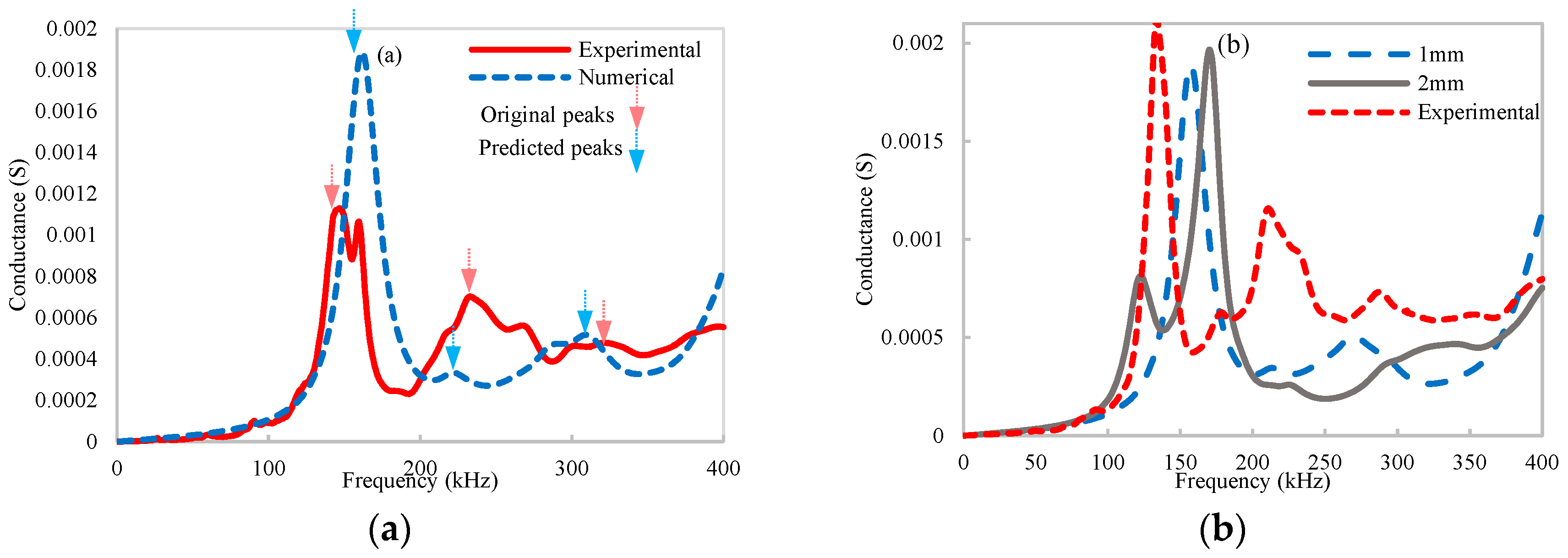
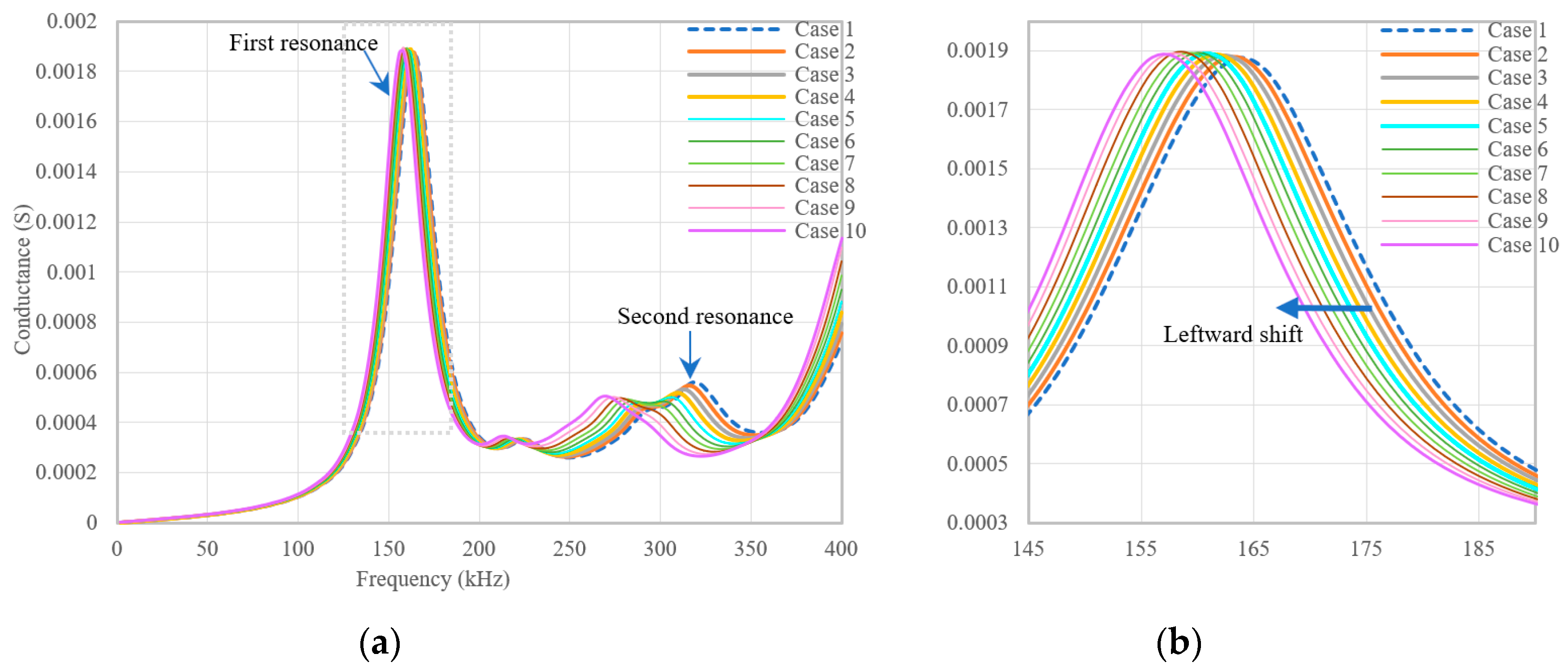
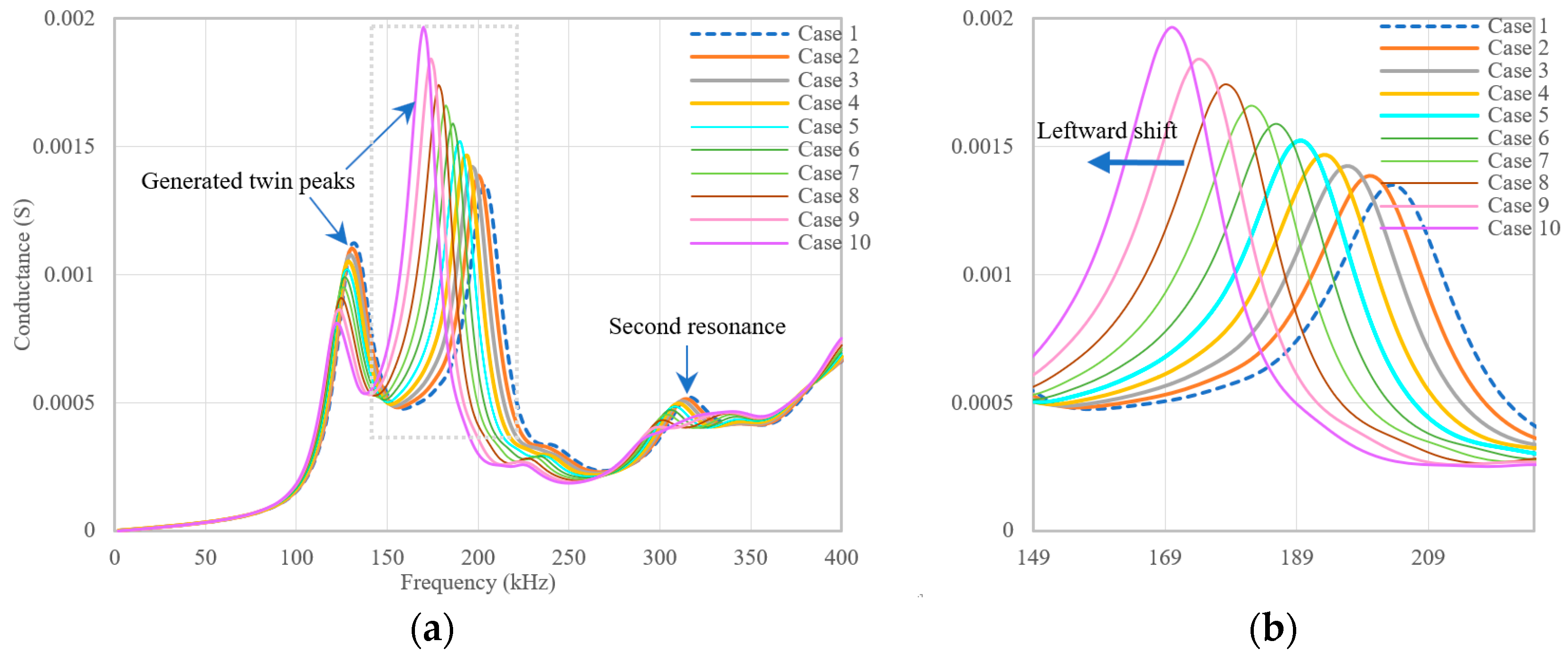
In the numerical modeling part, a 3D FE model for a concrete cube installed with an embedded PZT sensor was generated and employed for thermal transmission analysis from 30 °C to 60 °C. The modeling results demonstrated that (1) the heat transfer progress amplifies the temperature-induced EMA variations, where resonance peaks in conductance spectra shift with a frequency reduction and magnitude increment. (2) The maximum frequency shift and RMSD index of the sensor with a thin coat are magnified in comparison with those of the sensor with a thick one (6.5 and 5.4 times in this study, respectively) at the end of heating, which reveals significant aggravation of the thermal hysteresis effect by an increase in coat thickness.

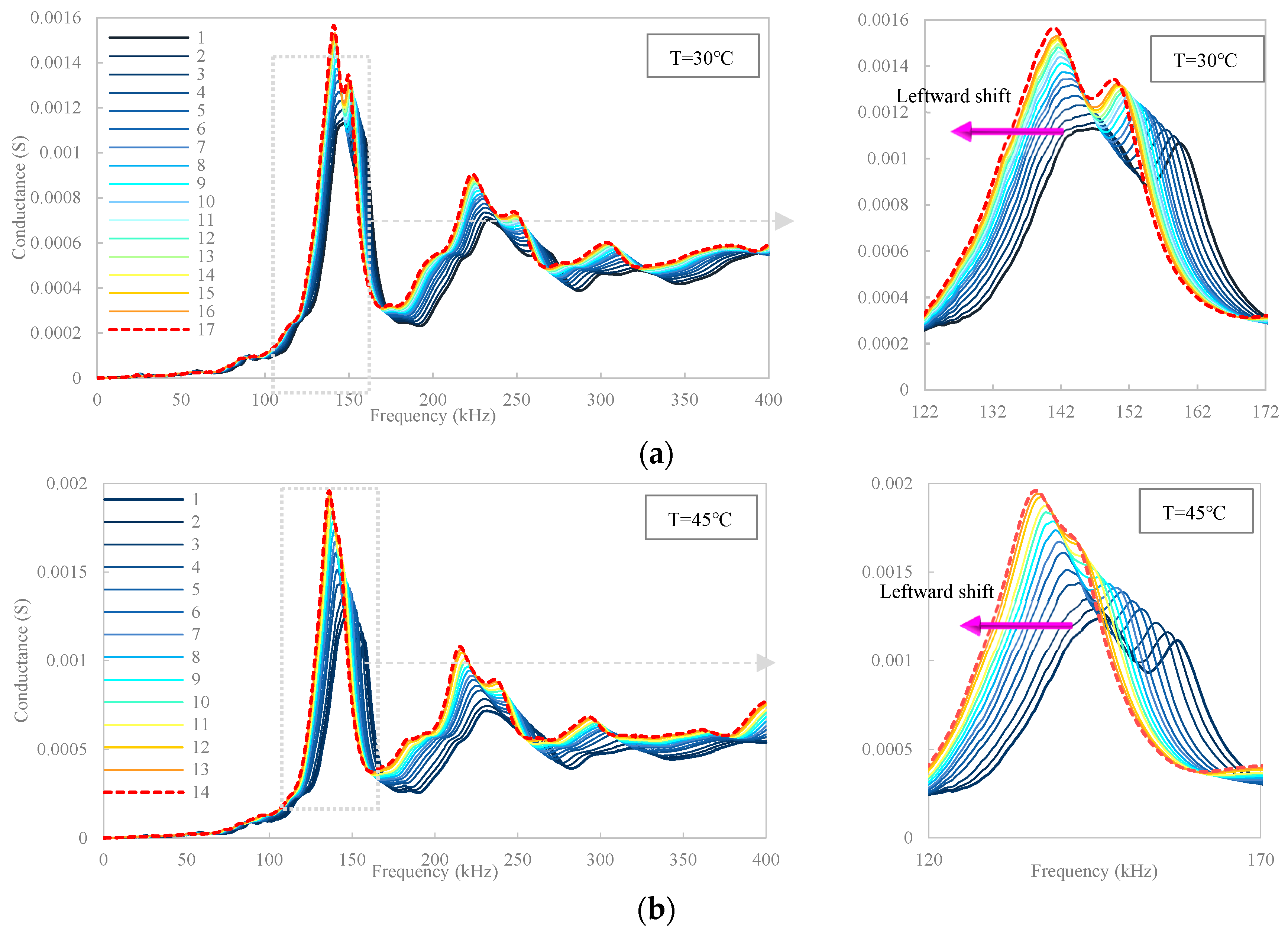
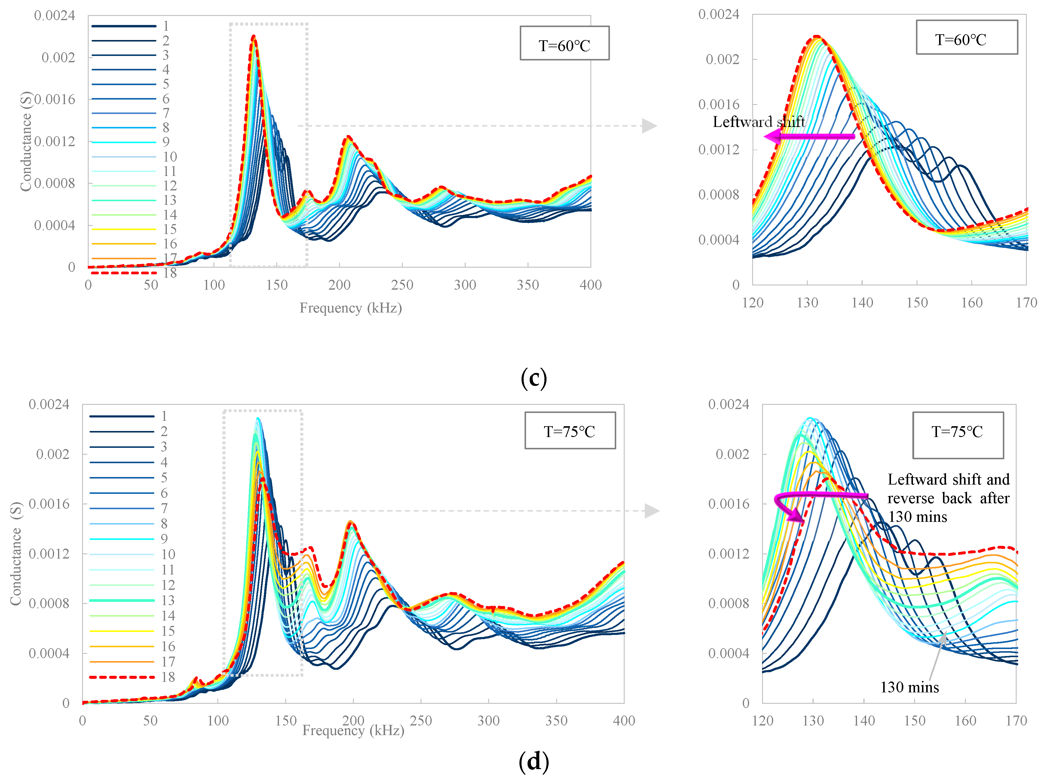
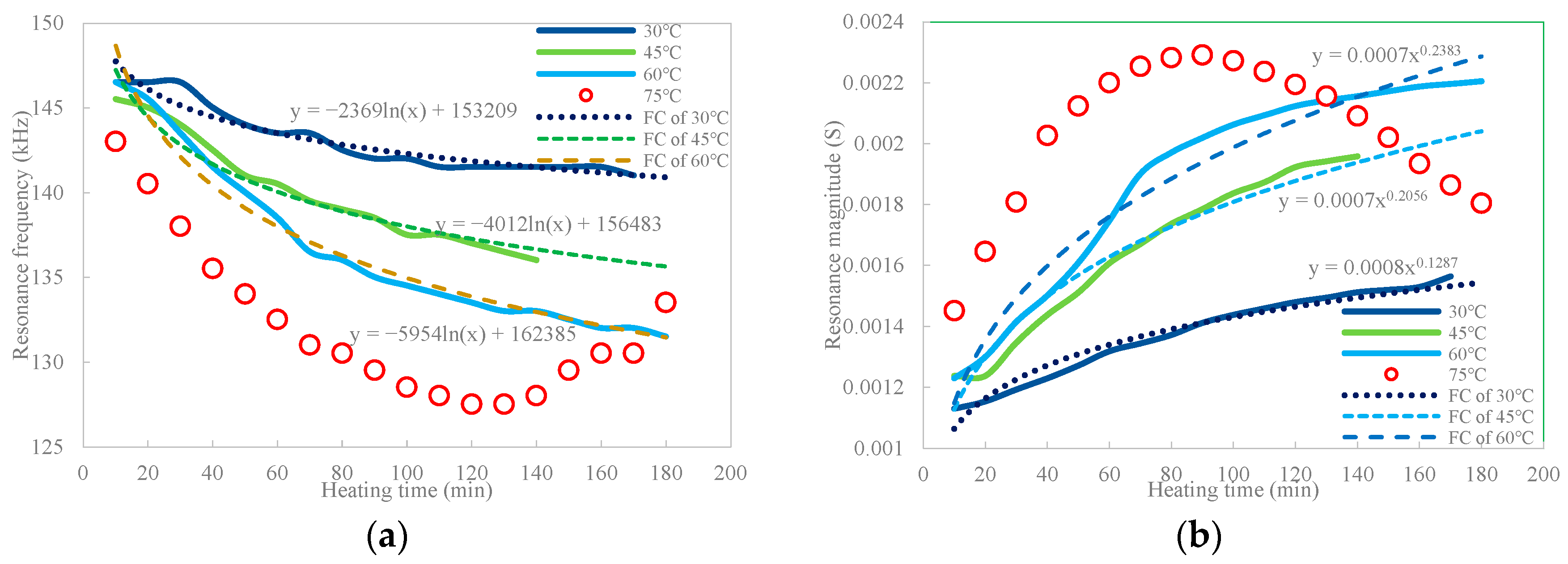
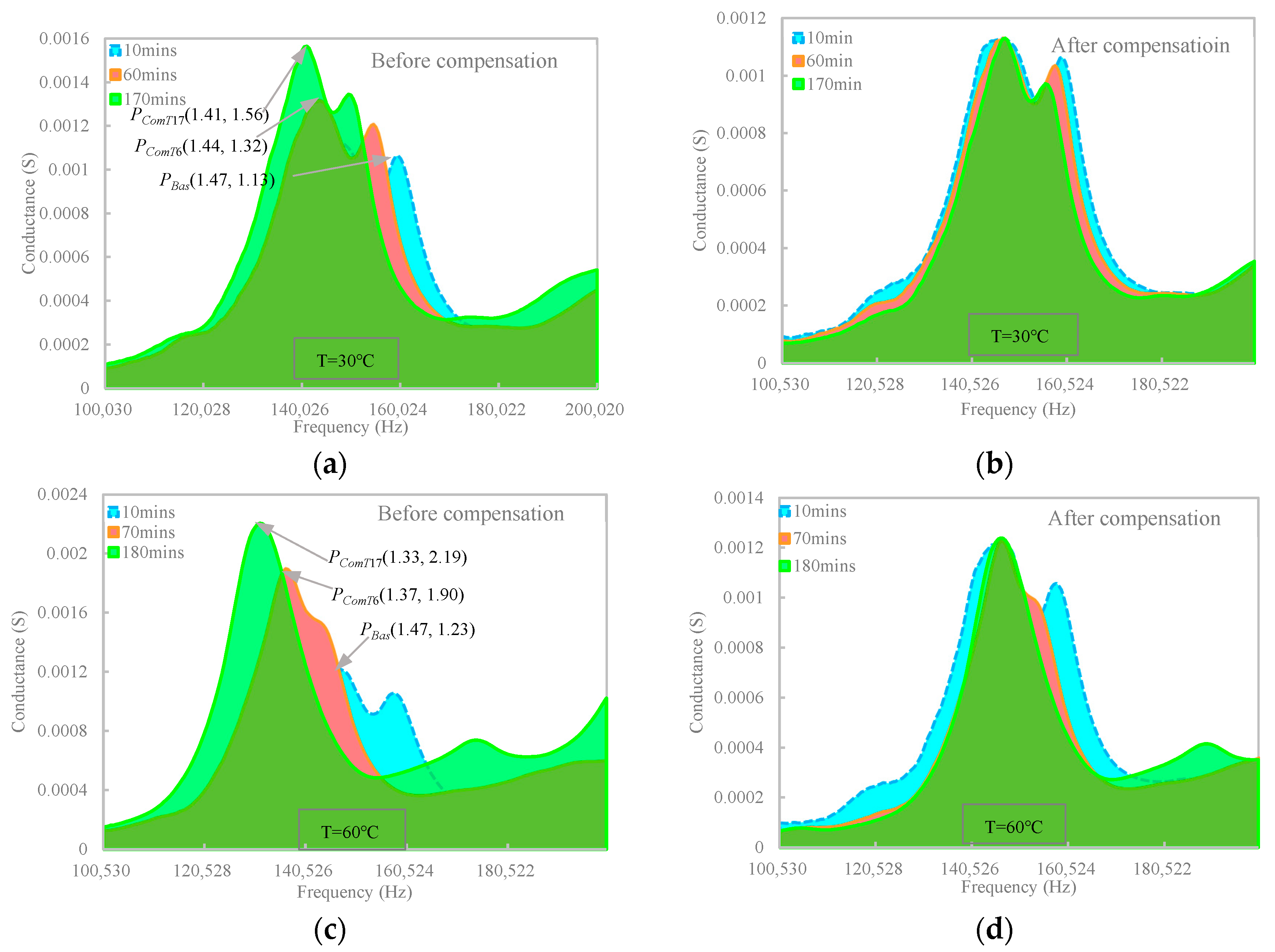
In the experimental investigation, a concrete cube installed with a CEP sensor was cast for a thermal test, which was heated for 180 min at four elevated temperatures of 30 °C, 45 °C, 60 °C, and 75 °C, respectively. Experimental results, as a cogent validation of the numerical results, indicated that (1) the heat transfer progress mainly causes gradual leftward and upward shifts in the resonance peaks of the EMA spectra in all temperature cases, which are amplified by temperature elevation. (2) Phase frequency and resonance amplitude aligned with heat transfer time were found to be in accordance with the negative Napierian logarithm and positive power functions, respectively. (3) Quantification of the EMA variation using RMSD/RMSDk indices also satisfied the Napierian logarithm and the power-function. (4) Anomalies in the resonance frequency and amplitude behaviors at a temperature of 75 °C indicated that potential distortion of EMA spectra of embedded PZT transducer could be induced by high-temperature generation. (5) Furthermore, a new methodology using frequency and magnitude shifts of the maximum resonance peak was attempted to compensate for the thermal hysteresis effect. Compensating results indicated that the conductance area increment induced by heating growth was significantly reduced by approximately 6 and 7 times for the two selected temperatures, which is promising for future applications.

Although promising results were attained, there are still limitations. (i) Since an anomaly in the resonance frequency and amplitude behaviors was observed at a temperature of 75 °C, the limited temperature range in this study warrants more investigations into the behavior of the embedded PZT patch under a wider range of extremely high temperatures. (ii) Inconsistencies that existed in some resonance peaks of the signatures after compensation also left a gap for improving the robustness of the proposed algorithm, relying on extensional tests under extreme temperatures. (iii) The proposed compensation technique is likely not suitable for compensation under minor temperature fluctuations due to the randomness of resonance peaks, particularly when encountering complex situations mixed with structural damage. (iv) Compensating for the extreme high-temperature effect in the EMA technique is also worth further investigation. (v) Some loss of valuable information may occur merely based on the CC indicator-based assessment for compensation, and accordingly, new indicators are supposed to be built up to evaluate the compensation effect in a more comprehensive way. (vi) Extending the approach into practice still faces the challenge that baseline data of EMA measurements might not be always available in real-world scenarios, hence developing a baseline-free compensation method may be more useful in practice.

References

1. Gao, L.; Thostenson, E.T.; Zhang, Z.; Chou, T.W. Coupled carbon nanotube network and acoustic emission monitoring for sensing of damage development in composites. Carbon 2009, 47, 1381–1388. [Google Scholar] [CrossRef]
2. Lim, A.S.; Melrose, Z.R.; Thostenson, E.T.; Chou, T.W. Damage sensing of adhesively-bonded hybrid composite/steel joints using carbon nanotubes. Compos. Sci. Technol. 2011, 71, 1183–1189. [Google Scholar] [CrossRef]
3. Sam-Daliri, O.; Faller, L.M.; Farahani, M.; Roshanghias, A.; Araee, A.; Baniassadi, M.; Zangl, H. Impedance analysis for condition monitoring of single lap CNT-epoxy adhesive joint. Int. J. Adhes. Adhes 2019, 88, 59–65. [Google Scholar] [CrossRef]
4. Stetco, C.; Sam-Daliri, O.; Faller, L.M.; Zangl, H. Piezocapacitive sensing for structural health monitoring in adhesive joints. In Proceedings of the 2019 IEEE International Instrumentation and Measurement Technology Conference, Auckland, New Zealand, 20–23 May 2019. [Google Scholar]
5. Soh, C.K.; Bhalla, S. Calibration of piezo-impedance transducers for strength prediction and damage assessment of concrete. Smart Mater. Struct. 2005, 14, 671–684. [Google Scholar] [CrossRef]
6. Ai, D.; Luo, H.; Zhu, H. Numerical and experimental investigation of flexural performance on pre-stressed concrete structures using electromechanical admittance. Mech. Syst. Signal Process. 2019, 128, 244–265. [Google Scholar] [CrossRef]
7. Lu, X.; Lim, Y.Y.; Izadgoshasb, I.; Soh, C.K. Strength development monitoring and dynamic modulus assessment of cementitious materials using EMI-Miniature Prism based technique. Struct. Health Monit. 2020, 19, 373–389. [Google Scholar] [CrossRef]
8. Ai, D.; Luo, H.; Wang, C.; Zhu, H. Monitoring of the load-induced RC beam structural tension/compression stress and damage using piezoelectric transducers. Eng. Struct. 2018, 154, 38–51. [Google Scholar] [CrossRef]
9. Sirohi, J.; Chopra, I. Fundamental understanding of piezoelectric strain sensors. J. Intell. Mater. Syst. Struct. 2000, 11, 246–257. [Google Scholar] [CrossRef]
10. Na, W.S.; Baek, J. A review of the piezoelectric electromechanical impedance based structural health monitoring technique for engineering structures. Sensors 2018, 18, 1307. [Google Scholar] [CrossRef]
11. Park, G.; Kabeya, K.; Cudney, H.H.; Inman, D.J. Removing effects of temperature changes from piezoelectric impedance-based qualitative health monitoring. In Proceedings of the Society of Photo-Optical Instrumentation Engineers of the Conference, San Diego, CA, USA, 21 July 1998. [Google Scholar]
12. Park, G.; Kabeya, K.; Cudney, H.H.; Inman, D.J. Impedance-based structural health monitoring for temperature varying applications. JSME Int. J. Ser. A-Solid Mech. Mat. Eng. 1999, 42, 249–258. [Google Scholar] [CrossRef]
13. Sepehry, N.; Shamshirsaz, M.; Bastani, A. Experimental and theoretical analysis in impedance-based structural health monitoring with varying temperature. Struct. Health Monit. 2010, 10, 573–585. [Google Scholar] [CrossRef]
14. Sepehry, N.; Bakhtiari-Nejad, F.; Shamshirsaz, M. Thermo-electro-mechanical impedance based structural health monitoring of plates. Compos. Struct. 2014, 116, 147–164. [Google Scholar] [CrossRef]
15. Freitas, E.S.; Baptista, F.G. Experimental analysis of the feasibility of low-cost piezoelectric diaphragms in impedance-based SHM applications. Sens. Actuators A-Phys. 2016, 238, 220–228. [Google Scholar] [CrossRef]
16. Ilg, J.; Rupitsch, S.J.; Lerch, R. Impedance-based temperature sensing with piezoceramic devices. IEEE Sens. J. 2016, 13, 2442–2449. [Google Scholar] [CrossRef]
17. Yang, Y.; Lim, Y.Y.; Soh, C.K. Practical issues related to the application of the electromechanical impedance technique in the structural health monitoring of civil structures: I. Experiment. Smart Mater. Struct. 2008, 17, 035008. [Google Scholar] [CrossRef]
18. Baptista, F.G.; Budoya, D.E.; Almeida, V.A.D.; Ulson, J.A.C. An experimental study on the effect of temperature on piezoelectric sensors for impedance-based structural health monitoring. Sensors 2014, 14, 1208–1227. [Google Scholar] [CrossRef] [PubMed]
19. Wandowski, T.; Malinowski, P.H.; Ostachowicz, W.M. Temperature and damage influence on electromechanical impedance method used for carbon fibre-reinforced polymer panels. J. Intell. Mater. Syst. Struct. 2016, 28, 782–798. [Google Scholar] [CrossRef]
20. Yang, Y.; Lim, Y.Y.; Soh, C.K. Practical issues related to the application of the electromechanical impedance technique in the structural health monitoring of civil structures: II. Numerical verification. Smart Mater. Struct. 2008, 17, 035009. [Google Scholar] [CrossRef]
21. Djemana, M.; Hrairi, M. Modeling and simulation of impedance-based damage monitoring of structures. Int. J. Simul. Model. 2016, 15, 395–408. [Google Scholar] [CrossRef]
22. Bhalla, S.; Soh, C.K. Structural health monitoring by piezo-impedance transducers. II: Applications. J. Aerosp. Eng. 2004, 17, 166–175. [Google Scholar] [CrossRef]
23. Grisso, B.L.; Inman, D.J. Temperature corrected sensor diagnostics for impedance-based SHM. J. Sound Vibr. 2010, 329, 2323–2336. [Google Scholar] [CrossRef]
24. Bastani, A.; Amindavar, H.; Shamshirsaz, M.; Sepehry, N. Identification of temperature variation and vibration disturbance in impedance-based structural health monitoring using piezoelectric sensor array method. Struct. Health Monit. 2012, 11, 305–314. [Google Scholar] [CrossRef]
25. Rabelo, D.D.; Steffen, V.; Neto, R.M.F.; Lacerda, H.B. Impedance-based structural health monitoring and statistical method for threshold-level determination applied to 2024-T3 aluminum panels under varying temperature. Struct. Health Monit. 2017, 16, 368–381. [Google Scholar]
26. Sepehry, N.; Shamshirsaz, M.; Abdollahi, F. Temperature variation effect compensation in impedance-based structural health monitoring using neural networks. J. Intell. Mater. Syst. Struct. 2011, 22, 1975–1982. [Google Scholar] [CrossRef]
27. Koo, K.Y.; Park, S.; Lee, J.J.; Yun, C.B. Automated impedance-based structural health monitoring incorporating effective frequency shift for compensating temperature effects. J. Intell. Mater. Syst. Struct. 2009, 20, 367–377. [Google Scholar] [CrossRef]
28. Huynh, T.C.; Kim, J.T. Compensation of temperature effect on impedance responses of PZT interface for prestress-loss monitoring in PSC girders. Smart. Struct. Syst. 2016, 17, 881–901. [Google Scholar] [CrossRef]
29. Gianesini, B.M.; Cortez, N.E.; Antunes, R.A.; Vieira, J. Method for removing temperature effect in impedance-based structural health monitoring systems using polynomial regression. Struct. Health Monit. 2020, 20, 202–218. [Google Scholar] [CrossRef]
30. Giurgiutiu, V.; Xu, B.; Liu, W. Development and testing of high-temperature piezoelectric wafer active sensors for extreme environments. Struct. Health Monit. 2010, 9, 513–525. [Google Scholar] [CrossRef]
31. Kamas, T.; Poddar, B.; Lin, B.; Yu, L. Assessment of temperature effect in structural health monitoring with piezoelectric wafer active sensors. Smart. Struct. Syst. 2016, 16, 835–851. [Google Scholar] [CrossRef]
32. Haider, M.F.; Giurgiutiu, V.; Lin, B.; Yu, L. Irreversibility effects in piezoelectric wafer active sensors after exposure to high temperature. Smart Mater. Struct. 2017, 26, 095019. [Google Scholar] [CrossRef]
33. Wandowski, T.; Malinowski, P.H.; Ostachowicz, W.M. Delamination detection in CFRP panels using EMI method with temperature compensation. Compos. Struct. 2016, 151, 99–107. [Google Scholar] [CrossRef]
34. Neville, A.M. Properties of Concrete, 4th ed.; John Wiley & Sons: New York, NY, USA, 1995. [Google Scholar]
35. Xu, D.; Sourav, B.; Wang, Y.; Huang, S.; Cheng, X. Temperature and loading effects of embedded smart piezoelectric sensor for health monitoring of concrete structures. Constr. Build. Mater. 2015, 76, 187–193. [Google Scholar] [CrossRef]
36. Ai, D.; Lin, C.; Luo, H.; Zhu, H. Temperature effect on electromechanical admittance-based concrete structural health monitoring. Struct. Health Monit. 2020, 19, 661–692. [Google Scholar] [CrossRef]
37. Ai, D.; Yang, Z.; Li, H.; Zhu, H. Heating-time effect on electromechanical admittance of surface-bonded PZT sensor for concrete structural monitoring. Measurement 2021, 184, 109992. [Google Scholar] [CrossRef]
38. Liang, C.; Sun, F.P.; Rogers, C.A. Coupled electro-mechanical analysis of adaptive material systems-determination of the actuator power consumption and system energy transfer. J. Intell. Mater. Syst. Struct. 1994, 5, 12–20. [Google Scholar] [CrossRef]
39. Annamdas, V.G.M.; Soh, C.K. Embedded piezoelectric ceramic transducers in sandwiched beams. Smart Mater. Struct. 2006, 15, 538–549. [Google Scholar] [CrossRef]
40. Ai, D.; Zhu, H.; Luo, H.; Wang, C. Mechanical impedance based embedded piezoelectric transducer for reinforced concrete structural impact damage detection: A comparative study. Constr. Build. Mater. 2018, 165, 472–483. [Google Scholar] [CrossRef]
41. Minh, P.V.; Thai, L.M.; Dung, N.T.; Tounsi, A.; Nhung, N.T.C.; Thom, D.V. An overview of the flexoelectric phenomenon, potential applications, and proposals for further research directions. Int. J. Mech. Mater. Des. 2023. [Google Scholar] [CrossRef]
42. Thai, L.M.; Luat, D.T.; Phung, V.B.; Minh, P.V.; Thom, D.V. Finite element modeling of mechanical behaviors of piezoelectric nanoplates with flexoelectric effects. Arch. Appl. Mech. 2022, 92, 163–182. [Google Scholar] [CrossRef]
43. Duc, D.H.; Thom, D.V.; Cong, P.H.; Minh, P.V.; Nguyen, N.X. Vibration and static buckling behavior of variable thickness flexoelectric nanoplates. Mech. Based Des. Struct. 2022. [Google Scholar] [CrossRef]
44. Dung, N.T.; Minh, P.V.; Hung, H.M.; Tien, D.M. The third-order shear deformation theory for modeling the static bending and dynamic responses of piezoelectric bidirectional functionally graded plates. Adv. Mater. Sci. Eng. 2021, 2021, 5520240. [Google Scholar] [CrossRef]
45. Moveni, S. Finite Element Analysis: Theory Application with ANSYS, 2nd ed.; Pearson Education Inc: Upper Saddle River, NJ, USA, 2003. [Google Scholar]
46. Ai, D.; Lin, C.; Zhu, H. Embedded piezoelectric transducers based early-age hydration monitoring of cement concrete added with accelerator/retarder admixtures. J. Intell. Mater. Syst. Struct. 2021, 32, 847–866. [Google Scholar] [CrossRef]
47. Annamdas, V.G.M.; Radhika, M.A. Electromechanical impedance of piezoelectric transducers for monitoring metallic and non-metallic structures: A review of wired, wireless and energy-harvesting methods. J. Intell. Mater. Syst. Struct. 2013, 24, 1021–1042. [Google Scholar] [CrossRef]
48. Xia, Y.; Xu, Y.; Wei, Z.; Zhu, H.; Zhou, X. Variation of structural vibration characteristics versus non-uniform temperature distribution. Eng. Struct. 2011, 33, 146–153. [Google Scholar] [CrossRef]
49. Krishnamurthy, K.; Lalande, F.; Rogers, C.A. Effects of temperature on the electrical impedance of piezoelectric sensors. In Proceedings of the Smart Structures and Integrated Systems, San Diego, CA, USA, 1 May 1996. [Google Scholar]
Figure 1. A model of PZT patch subjected to voltage excitation in its thickness vibration.
Buildings 13 02564 g001
Figure 2. Model of embedded PZT transducer coated by adhesive in cement mortar and structure.
Buildings 13 02564 g002
Figure 3. (a) FE model of FVP; (b) numerical and experimental conductance spectra of the FVP.
Buildings 13 02564 g003
Figure 4. 3D FE model of a half concrete cube installed with embedded PZT sensor.
Buildings 13 02564 g004
Figure 5. Comparison of numerical and experimental conductance spectra of PZT embedded inside the concrete cube under (a) 30 °C and (b) 60 °C.
Buildings 13 02564 g005
Figure 6. Layered concrete cube with embedded PZT model for thermal transmission analysis.
Buildings 13 02564 g006
Figure 7. Evolution of conductance signatures in frequency band of (a) 0–400 kHz, (b) 145–190 kHz for embedded PZT sensor with 1 mm coat layer in concrete cube under heating.
Buildings 13 02564 g007
Figure 8. Evolution of conductance signatures in frequency band of (a) 0–400 kHz, (b) 149–215 kHz for embedded PZT sensor with 2 mm coat layer in concrete cube under heating.
Buildings 13 02564 g008
Figure 9. (a) Resonance frequency shift, (b) RMSD index of conductance signatures of PZT patch with 1 mm/2 mm adhesive layer embedded in the concrete cube under heating.
Buildings 13 02564 g009
Figure 10. Manufacturing steps for the CEP transducer and experimental layout for the thermal hysteresis effect test.
Buildings 13 02564 g010
Figure 11. (a) Conductance, (b) susceptance signatures obtained from FVP patch and CEP transducer.
Buildings 13 02564 g011
Figure 12. Evolution of conductance signature within 0–400 kHz and magnified within 120–170 kHz for the cube heated for 180 min at (a) 30 °C, (b) 45 °C, (c) 60 °C, and (d) 75 °C.
Buildings 13 02564 g012aBuildings 13 02564 g012b
Figure 13. FCs of (a) phase frequency and (b) amplitude response with heat transfer time of the first resonance in the conductance signatures at different temperatures.
Buildings 13 02564 g013
Figure 14. FCs of the (a) RMSD and (b) RMSDk indices versus heat transfer time at different temperature conditions.
Buildings 13 02564 g014
Figure 15. Conductance of CEP installed in the concrete cube at temperature of 30 °C (a) before and (b) after compensation, and 60 °C (c) before and (d) after compensation.
Buildings 13 02564 g015
Figure 16. CCD index for the conductance measured at temperature of (a) 30 °C and (b) 60 °C when heated for 70 and 180 min before and after compensation.
Buildings 13 02564 g016