Abstract
Damage identification plays an important role in enhancing resilience by facilitating precise detection and assessment of structural impairments, thereby strengthening the resilience of critical infrastructure. A current challenge of vibration-based damage detection methods is the difficulty of enhancing the precision of the detection results. This problem can be approached through improving the noise reduction performance of algorithms. A novel method based partially on the errors-in-variables (EIV) model and its total least-squares (LS) algorithm is proposed in this study. Compared with a classical damage detection approach involving adoption of auto-regressive (AR) models and the least-squares (LS) method, the proposed method accounts for all the observation errors as well as the relationships between them, especially in an elevated level of noise, which leads to a better accuracy. Accordingly, a shaking table test and its corresponding finite element simulation of a full-scale web steel structure were conducted. The acceleration time-series output data of the model after suffering from different seismic intensities were used to identify damage using the presented detection method. The response and identification results of the experiment and the finite element analysis are consistent. The finding of this paper indicated that the presented approach is capable of detecting damage with a higher accuracy, especially when the signal noise is high.
1. Introduction
Structures are subjected to diverse types of adverse factors such as earthquakes, hurricanes, explosions, and overcapacity loads, leading to evitable damages [1]. Damage identification is crucial for enhancing resilience through timely detection and assessment of impairments in systems [2]. By integrating advanced sensing technologies, data analysis, and decision support systems, people can make informed decisions, optimize resource allocation, and enhance the resilience of critical infrastructure in the face of unforeseen events or operational challenges [3,4]. Aiming at enhancing structural resilience, many techniques have been used to study structural performance after damage. Over the past several decades, damage detection methods such as the finite difference method, finite element (FE) simulations and analysis, and experiments such as shaking table model tests [5,6,7,8] have been reported in the literature. Research on the shaking table test and the corresponding FE analysis has reported on the dynamic responses and seismic performance of structures [9]. Based on these results, the engineering community has also explored damage detection methods [5], which have been used to deal with observational and output data such as displacements, accelerations, and the natural frequencies of shaking table tests and FE simulations.
The vibration-based damage evaluation method has received considerable attention for its noninvasive and uncomplicated characteristics [10,11], especially popular in the shaking table test model. The mechanism of these approaches involves the observation of the structural mode, frequencies, or time series output over time, the extraction of sensitive damage features, and the evaluation of structural damages [12]. Vibration-based damage detection can be divided into frequency-domain-based methods and time-domain-based methods and their combination. As for frequency-domain based methods, He et al. [13] carried out shaking table tests on two concrete shear wall model structures and the test of complete uniaxial compressive constitutive curves of concrete. Moaveni et al. [14] conducted a full-scale shaking table test of a reinforced concrete building section and found that three damage identification methods used in the experiment did not exactly coincide. As for time-domain-based methods, Li et al. [15] studied the performance of a high-rise building through the shaking table test and its corresponding FE simulations. The damage levels and distributions of the model building were successfully identified based on the observations in the experiment. In addition, some research investigated effective damage detection methods including vibration-based methods, and they have been successfully applied to detecting and identifying the damages in structures constructed from various types of materials, such as reinforced concrete [16], steel [17], and composites [18]. Morita et al. [19] detected and estimated the damage of steel frames through a shaking table test by two identification methods.
One of the most commonly used time-domain-based techniques, a method based on the auto-regressive (AR) model, has also been applied in a variety of engineering applications [20]. The AR model can account for correlations between the current time parameter with its predecessors in the time series [21]. In this model, the output variable depends linearly on its previous values and a stochastic term, which means errors only exist in the current observations. Damage levels in a structure can be identified by AR coefficients between the undamaged structure and the structures to be detected [22]. The famous least-squares (LS) method is one of the most commonly used methods for estimating parameters such as the structural damage indicators in the AR model [23].
However, some research has pointed out that the classical AR model ignored the errors of previous observations, which introduced errors in the evaluated AR parameters, and led to biased results [24]. Zeng [25] proved and quantified the negligible differences in the estimated parameters caused by the LS solution and the classical AR model. To deal with this defect, a large variety of bias-compensated LS methods have recently been proposed in the past few years. For instance, Diversi et al. [26] proposed a new and effective identification method considering the AR model with additive noise. Esfandiari et al. [27] presented four new methods for estimating the parameters of an autoregressive (AR) process based on observations corrupted by white noise. One can notice that the AR model with noise is actually the well-known errors-in-variables (EIV) model in the field of geodesic surveys [28]. Among the various solutions for the EIV model, total least-squares (TLS)-based algorithms indicate better accuracy compared with the classical LS solution [29]. Hence, new parameter estimation methods based on the AR model plus noise, based on the extensive achievements in geodesic surveys, may potentially be applied to the field of structural damage detection.
To overcome the current limitations of damage identification results based on AR models, which are greatly affected by environmental interference and prove ineffective in practical cases, this paper aims to propose a high anti-noise structural damage identification method that considers all errors in observations. Furthermore, the application effects of this method in real cases are thoroughly examined. In the proposed structural damage detection method, a TLS solution based partially on EIV model theory is applied to identify the parameters of the AR model with noise. A full-scale shaking table test of a two-story web steel structure is conducted to study its seismic performance. The proposed damage detection method is used to further identify the damage levels of the model under different earthquake intensities. The structure of this paper can be listed as follows. In Section 2, an AR model with noise and its parameter estimation method are introduced. This method considers not only the noise in current observations but also in past observations, and a sensitive damage indicator is also adopted to represent damage levels. In Section 3, the performance of the estimation method is analyzed based on a mathematical simulation. Section 4 introduces the shaking table test and the corresponding FE simulation of the web steel structure. The results of the experiment, FE simulation, and damage detection are presented in Section 5. This study not only indicates that the light steel structure performs well in earthquakes, but also proves that the proposed damage identification method is effective in practice.
2. LS Adjustment for the AR Model with Additive Noise
2.1. AR Model with Additive Noise
A classical AR model of order is described by:
where is the discrete-time signal of the acceleration responses; is the possible random noise in ; is the model’s order, it varies from 0 to ; is unknown coefficient in the AR model and it is calculated by corresponding algorithms. In a practice conditions, when a structure operates under normal conditions, the noise can be assumed as the famous Gaussian white noise, this noise has a zero-mean and unknown variance [30].
In fact, the left term of the model can be seen as the sum of the two terms on the right. The first term considers to with unknown coefficients, while the second term represents the noise affection. Denote , , and . The AR model can be represented as:
where is the error corresponding to . Since is obtained by observation in practice, then vector as well as the matrix A should contain errors. In this regard, the existing errors in matrix A are neglected as a simplification in the classical AR model. However, errors should be added to matrix A in Equation (2), represented by . And the AR model can be rewritten as:
subject to
where and are diagonal weight matrices of and , respectively. Here, , which is the vector of putting the elements of into a vector one column after another; and .
Equation (4) is the well-known EIV model. Notice that in a special case when the matrix contains no errors , then the model is the classical AR model in Equation (2) with only noise . By comparing Equations (2) and (3), we can observe that Equation (3) includes an error term, EA, corresponding to the matrix A. EA represents all the errors present in the elements of matrix A. Since the elements of A are the previous observations, it is certain that they would contain errors caused by various factors such as manual operations, machine precision, and environmental influences. However, Equation (2) dismisses these errors. Consequently, these errors, combined with the algorithm based on Equation (2), can result in inaccuracies in the calculated coefficients. Particularly in situations with high noise levels, neglecting EA can lead to significant errors in parameter estimation, causing substantial deviations in the identification factor from the actual scenario.
As mentioned in the introduction, studies of the EIV model have been quite popular in the field of geodesic surveys and a lot of valuable results have already been reported. An extended, more general, EIV model called the partial EIV model proposed by Xu et al. [31,32] have been proposed. Not all the elements in the design matrix A are random in the partial EIV model. This model is represented as follows:
In Equation (5) ; is a deterministic constant vector whose elements are composed of non-random elements of ; is the symbol of the Kronecker product; is a vector with the size of , and with independent random entries in the design matrix A, it is also the true value of ; is a given matrix with the size of , it depends on random element numbers in the matrix ; and is a vector that represents the random component.
It is clear that the AR model with additive noise is a special case of the partial EIV model. When and , Equation (5) reduces to Equation (3), which is shown as follows:
The observations utilized for damage detection can be acquired from the same types of time-series. For example, accelerations are obtained by the same equipment in the same testing sites. Hence, the diagonal weight matrix in Equation (4) is assumed as the unit matrix. By evaluating the unknown vector of the partial EIV model, the coefficients of the AR model with additive noise can be obtained.
2.2. Existing TLS Solutions for the EIV Model
The solution for Equation (6) can be described as follows. Firstly, assuming that and are stochastically independent, that is,
The TLS solution is,
where , , and , , , , . ,,, are matrices, for , these matrices are, respectively, given by the following:
Based on this solution, an optimistic solution for the partial EIV model can be considered as an optimization problem. Thus, the cost function is rewritten as follows:
Finally, the solution is as follows:
where . The final solution can be obtained through an iterative process. The new solution may be more concise and straightforward compared to formulas (9) and (10). Specifically, the alternative approach is simpler and can be processed more efficiently when the number of independent random elements in the design matrix is considerably larger than the number of measurements.
2.3. TLS Solution for the Modified AR Model
It is clear that in the AR model plus noise, the same elements occur in and , which means that they should be not stochastically independent. Thus, simply assuming is not reasonable. This may lead to the solution above (Equations (13) and (14)) not being able to be used directly. In this work, this solution is still used, named as TLSp. The errors of in the are not assumed to be the same as the errors of in the , . That is, is not always the same as . Then, the solution above (Equations (13) and (14)) can be used for solving the AR model plus noise. Although should be the same as in true cases, the actual value of errors in is unknown. Thus and may be closer to true errors. In this regard, it is more appropriate to assume that and are not the same, and we should estimate them independently rather than disregarding these errors in matrix A. Under these assumptions, the TLSp parameter estimation steps of the AR model with additive noise are shown as follows,
- Given and , , ;
- Initialize ;
- Compute by Equation (13);
- Compute by Equation (14) based on the obtained in Step 3.
- Given a predetermined tolerable error value, if the errors between and are within the given value, terminate the estimation. Otherwise, go to Step 3.
The AIC criterion is used in this paper to determine the optimal order of the AR model, formulated as [33]:
where is the estimated variance of the residual errors of order n. N is the total number of samples.
2.4. Damage Detection Indicator
After obtaining the parameter of the AR model, a damage indicator can be introduced to indicate the damage degree of the structure. The differences in the indicators between in the healthy conditions with those of the damaged conditions cannot be measured simply by visual inspection, especially where numerous elements exist in . In this paper, the structural damages are represented by the ratio between the Euclidean distance of the undamaged with the damaged . The calculation steps are clarified as follows:
- 1
- The obtained response acceleration time-series data are divided into two parts, i.e., part and part , where is used as the baseline data and serves as the unknown data to be estimated when there is damage to the structure.
- 2
- Estimating and through Equations (12) and (13). The square of the Euclidean distance between with is calculated as:
- 3
- Estimating the of ith output data of the damaged structure through Equations (12) and (13). The Euclidean distance between and is calculated as,
- 4
- Finally, the damage indicator, named IF in this paper, is calculated as the ratio between and , as follows:
The IF should be close to 1 when the data to be estimated are acquired from an undamaged structure. As the damage level of the structure increases, the differences between the parameters of the undamaged structure and the damaged structure should increase, resulting in an increase in the IF value.
3. Performance Analysis
In this section, a mathematical simulation is used to analyze the performance of the damage detection method presented above. The estimation results of the adopted TLS method in Equations (13) and (14), and AR model with noise are studied carefully. A comparison between the traditional AR model with the corresponding LS solution and the AR model and the addition of noise with its TLS solution is demonstrated.
Taking the following 4th-order AR model as an example [26],
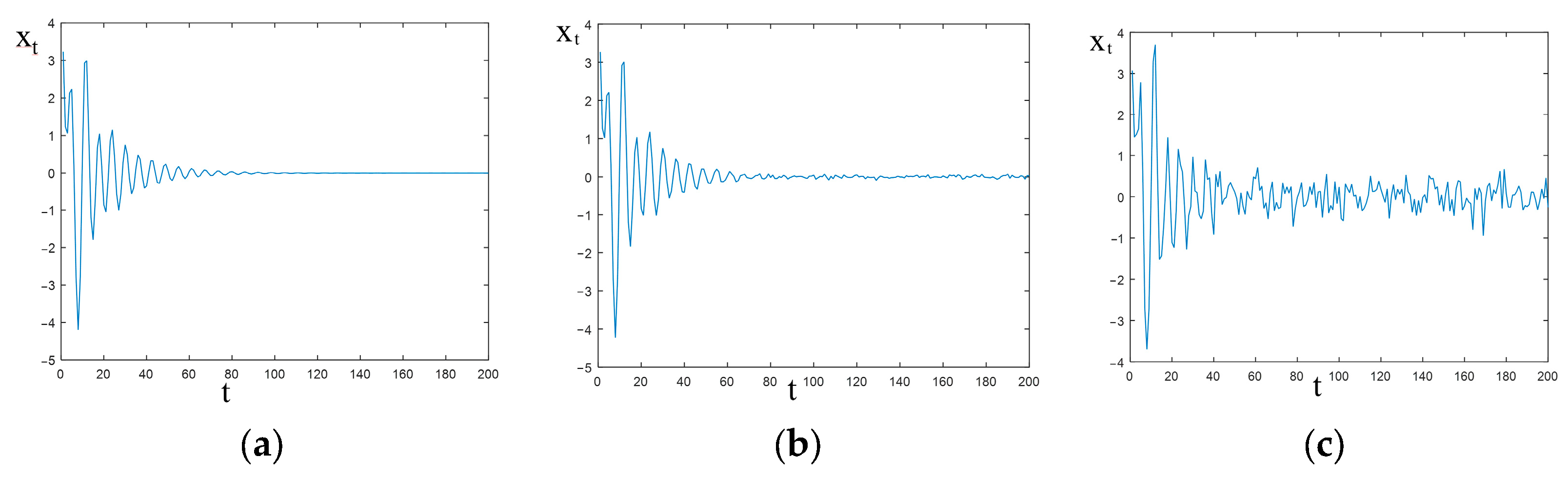
where is Gaussian white noise, i is the time sequence number. , and . The number of samples is limited to 200, and the Gaussian white noise series with different signal-to-noise ratios (SNR) are applied to the real time-series values . Six SNR conditions, 60 dB, 50 dB, 40 dB, 30 dB, 20 dB, and 10 dB, are simulated. Specifically, for each SNR, the elements in the noise series are the same. The real value of and with the error conditions of 30 dB and 10 dB are shown in Figure 1. The obtained for different SNR conditions is listed in Table 1.
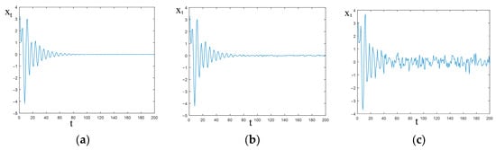
Figure 1.
Output time series: (a) real value; (b) SNR is 30 dB; (c) SNR is 10 dB.

Table 1.
Values of estimated parameters.
When , the AIC meets its minimum value. When there is no noise, the identification results are real values . More identification results with different SNR conditions are shown in Table 1. It is indicated that as the SNR = 60 dB, the solution of the LS estimation and the TLSp estimation are nearly the same and quite close to the real value, indicating both methods perform well in this condition. However, the differences between the two methods increase as the SNR rises. As for the condition of SNR 20 dB, the estimation results of the proposed model and algorithm are closer to the true value, while the LS solution differs more significantly. When the SNR is 10 dB, the results from both of the two methods contain large errors, The identification vector of TLSp, [2.2818, −2.6567, 1.5899, −0.4600], exhibits four elements that are relatively closer to the actual values compared to the four elements of the LS solution, which are [2.2017, −2.5084, 1.4482, −0.4064]. This comparison highlights the improved accuracy of the TLSp method in estimating the true values of the elements. Hence, it can be concluded that the parameter estimation method proposed in this paper performs better, even in the presence of strong noises.
It is clear that, as the SNR increases, the gaps between parameters of healthy and estimated stages become larger. Assuming that the changes in the parameters in Table 1 are not caused by different levels of errors, but by the different levels of inner damage of the system. For example, assume (SNR = 20 dB, TLSp) is estimated by the output signals of a damaged condition of a structure by the proposed method. Then, in order to measure the structural damage level, the damage indicator needs to be calculated to quantify the parameter changes to this system. Therefore, different levels of SNR represent different levels of gaps between the parameters of the healthy system, which can be estimated. The damage levels represented by the values of structures are expected to increase as the SNR values increase. The IFs of the example in Table 1 are shown in Table 2.
Table 2.
IFs of different conditions.
It is clear that the increases in the IFs values are related to the rising SNR, reflecting the effectiveness of the damage indicator. As for the same SNR, the IFs of the LS solution are larger than that of the TLSp solution. For example, when the SNR = 10 dB, the IFs of the LS solution are approximately twice as large as the IFs of the TLSp solution. Therefore, the TLSp solution outperforms the traditional LS solution.
4. Experimental and Numerical Techniques
A shaking table test of a two-story full-scale web steel model under seismic excitation with increasing intensities and the corresponding FE simulation is presented in this section.
4.1. Shaking Table Model Test
A full-scale model of a two-story web steel structure was subjected to a shaking table model test to investigate its seismic performance. The web steel originating from Canada is a type of cold-formed steel with a thin wall which has already been utilized in various countries. The model used in the experiment has dimensions of 2 m × 3 m and a total height of 6 m. Accelerations and displacements were measured using the DASP2003 dynamic signal acquisition and analysis system, developed by the China Orient Institute of Noise and Vibration. The dynamic strain was obtained using the DH3817 dynamic and static testing instrument. The data acquisition instrument can be seen in Figure 2, and a photo of the completed model structure is shown in Figure 3
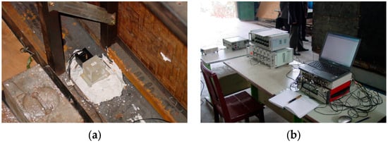
Figure 2.
Data acquisition instruments: (a) accelerometer; (b) signal acquisition device.
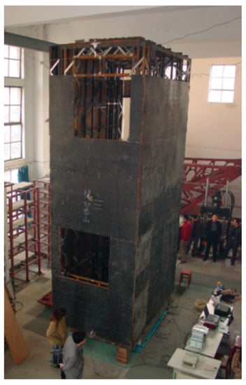
Figure 3.
Photo of the completed model.
The seismic excitation of the El Centro waves (1940, America), and the Qian’an waves (1976, China) with different intensity conditions are simulated on the shaking table model. The sequence of the experiment is shown in Table 3. As can be seen, there are five levels of tested earthquakes with the corresponding peak ground acceleration (PGA) values. The free vibration and the swept frequency method are conducted before the seismic test. Furthermore, white noise excitation is utilized before and after all of the groups of seismic activities to capture the output shifts due to the seismic induced damage. The sampling time interval is 3.905 ms. The seismic waves used in the experiments were unidirectional input excitations, with the peak accelerations corresponding to the seismic intensity values specified in the Chinese Code [34].
Table 3.
Sequence of the shaking table test.
The displacement is achieved by pulling the top of the structure with a certain degree of deflection, and then fixing the deflection, followed by an abrupt cutting of the rope, for the purpose of assessing the structure’s free vibrations. The measured response represents the characteristic free vibrations of the structure. The white noise excitation had a peak acceleration of 0.2 g and a duration of 40 s. The sweep frequency excitation, consisting of both upward and downward frequency sweeps, had peak accelerations of 29 g for each direction and a duration of 40 s. The peak accelerations of the excitation waves used in the experiment can be referred to in Table 3.
Five accelerometers were distributed around the model, with two on the top floor, two on the second floor and one on the first floor, shown in Figure 4. Three displacement sensors and eight strain gauges were used. The accelerometer distribution is shown in Figure 4. Point 1 is on the table surface, points 2 and 3 are on the second floor, and points 4 and 5 are on the top floor.
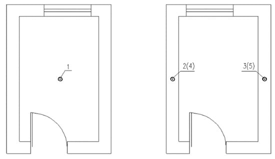
Figure 4.
Accelerometer distributions.
4.2. Finite Element Simulation
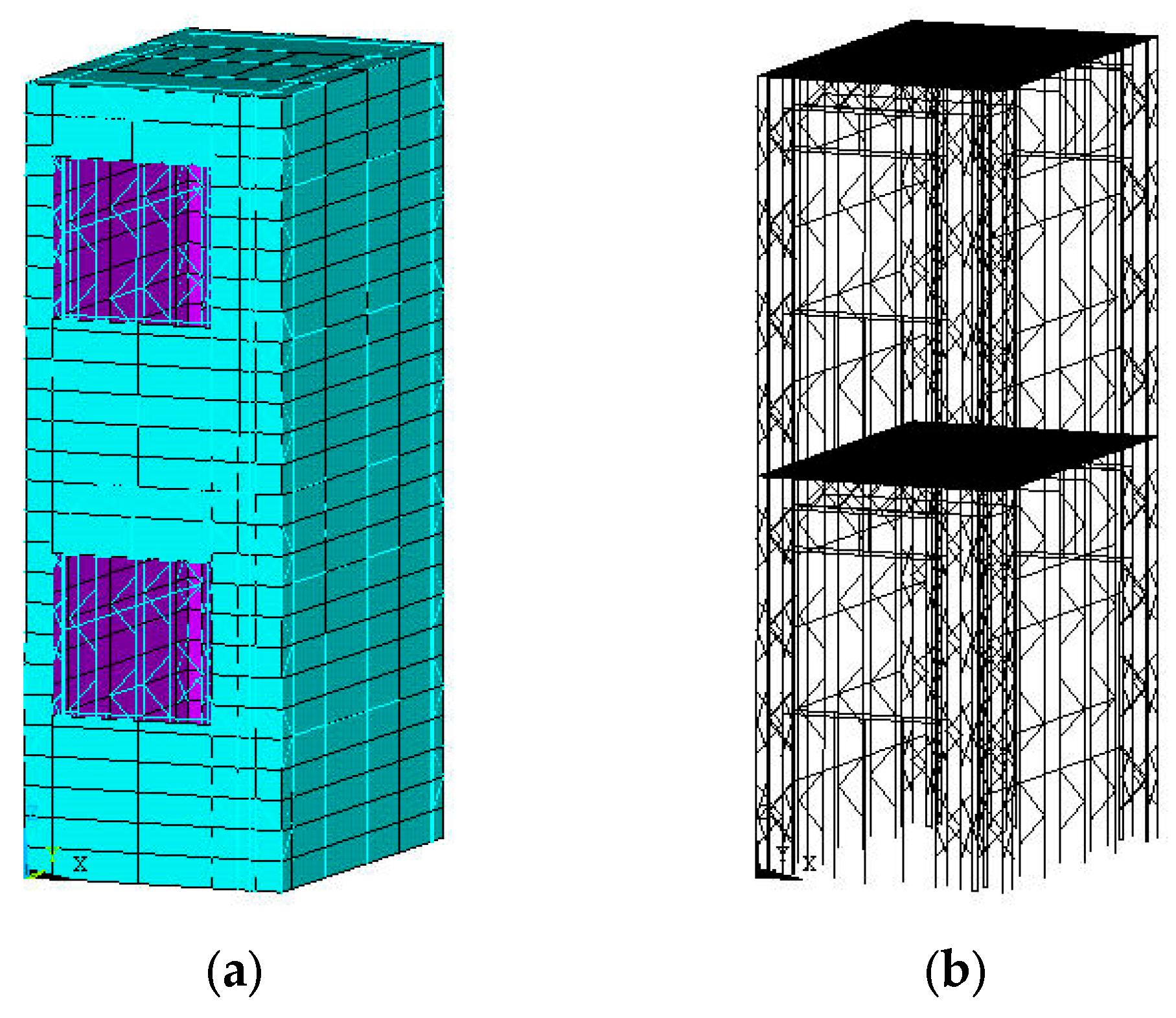
An FE simulation of the shaking table test was also conducted using ANSYS. The properties of the steel were determined by the experiment and the nonlinear performance was considered. The beam and shell elements were used to simulate the square steel tube and bamboo plywood. Properties of the main steel components in the web-steel structure are shown in Table 4. The steel strip and V fittings were simulated by bar elements. The steel strip only sustains tension. Other elements in the model are simulated by solid 70. There were approximately 11,500 nodes in total. The finite element model of the structure is shown in Figure 5.
Table 4.
Properties of the main steel components in the web steel structure.
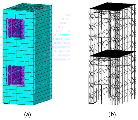
Figure 5.
The FE model: (a) total model; (b) skeleton model.
The testing conditions were consistent with the experiment. The input waves were simulated by the tested acceleration data recorded on the table surface. The input waves were simulated by the tested acceleration data recorded on the table surface. The frame foundation and nodes at the base of the columns were set as rigid joints. The boundary constraint types for the bottom three nodes of the frame columns were symmetry/antisymmetry/encastre. The encastre type boundary condition was selected to define the boundary condition at the bottom of the frame columns. According to the specific conditions of the structure, the grid size for the beam elements in the structure was 0.6 m, while the grid size for the shell elements and the solid elements was 0.3 m. The weight of the model was adjusted by the material density of the floor units to ensure that the self-weight of the simulation model was the same as that of the shaking table test model.
Firstly, modal analysis was performed to determine the natural frequencies of the structure based on the vibration tests. The dynamic response of the structure under earthquake excitations, such as the El Centro wave and the Qian’an wave, was then obtained by applying these excitations to the finite element model. The natural frequencies of the structure were calculated through frequency analysis, while the dynamic response under earthquake excitations was determined using the modal dynamics analysis module within linear perturbation analysis.
5. Experimental, Numerical, and Identification Results
In this section, the seismic performance of the model structure is studied. Based on the proposed damage detection method, the damage levels and distributions of the test model are identified using the output accelerations induced by white noise after different testing conditions.
5.1. Experimental Results and Analysis
The dynamic characteristics, such as the natural frequency, and the damping ratio are listed in Table 5. The web steel structure performed well when subjected to seismic waves in the experiment. No components were cracked or destroyed after all the testing earthquake waves were applied. All of the steel pipes, connections, and other construction members appear to remain in good condition. When the accelerations were small, such as 0.1 g, there were no visible responses or obvious sounds occurring. However, the model responds with squeaky sounds when accelerations increase to 0.3 g, which reflects tension and occlusion appearing in some joints, such as the connections between the bamboo plywood and steel pipes and inter-story connections. Therefore, it can be inferred that the structure has satisfactory energy dissipation capacity when suffering from seismic waves.
Table 5.
Dynamic characteristics of different excitations.
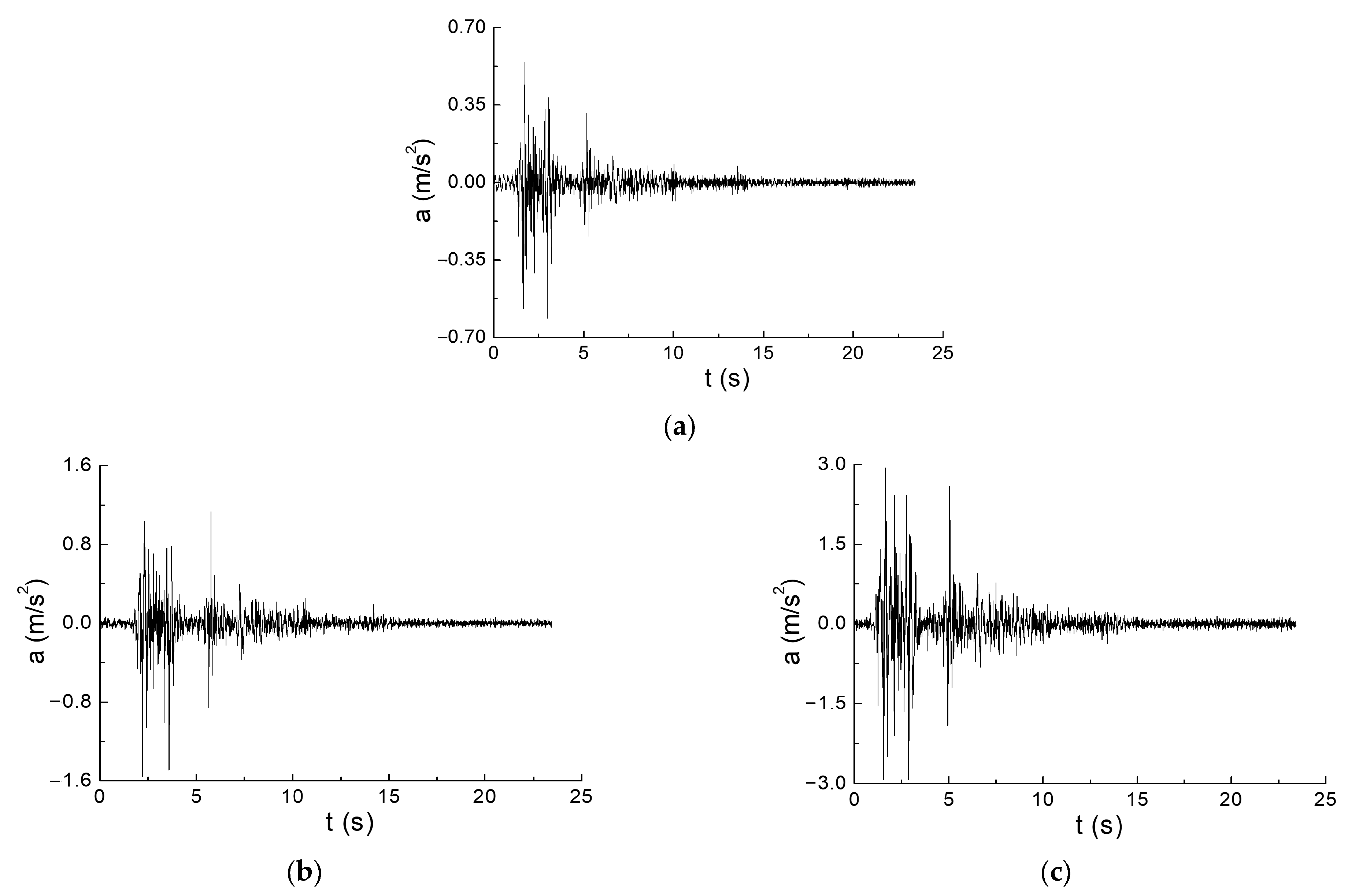
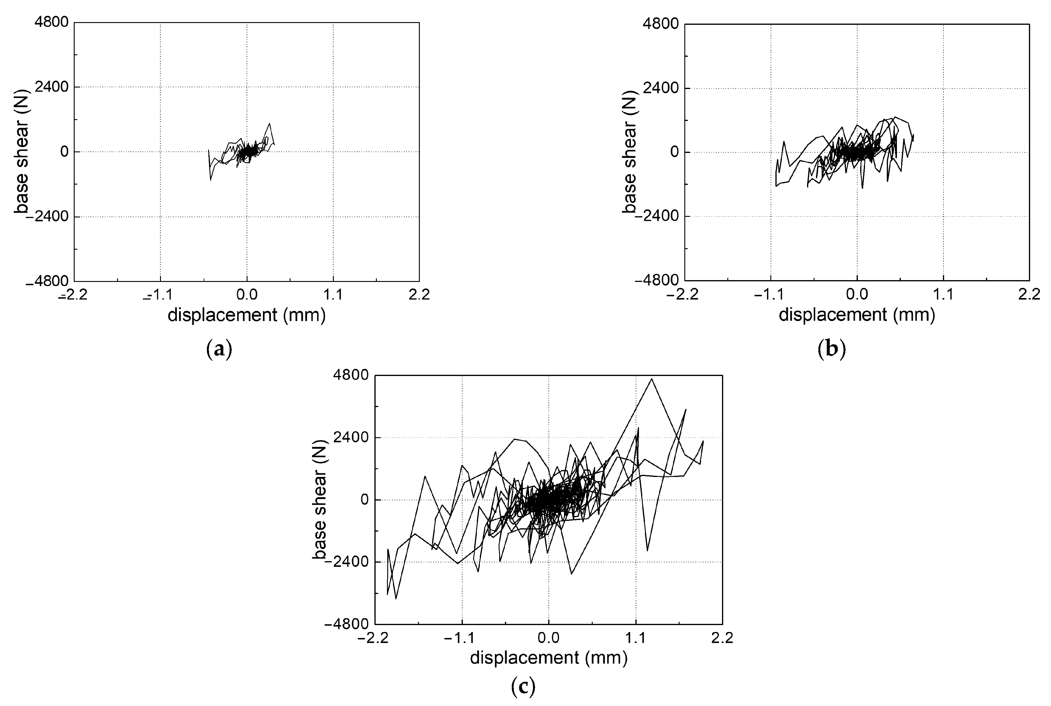
Representative peak acceleration and displacement responses of the model subjected to EI Centro waves and Qian’an waves under different testing conditions are shown in Table 6. The acceleration time–history curves of the top floor suffering from 0.1 g and 0.3 g EI Centro waves are shown in Figure 6. Figure 7 shows the relationship between the bottom shear and the second story displacement corresponding to EI Centro waves.
Table 6.
Peak responses of the model under different test conditions.
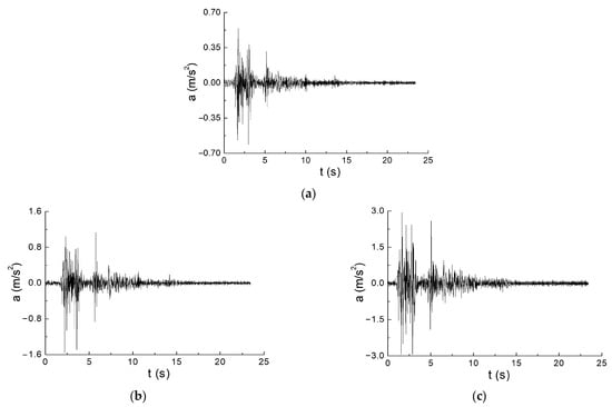
Figure 6.
Acceleration time–history curves of the top floor in response to EI Centro waves: (a) 0.1g; (b) 0.2 g; (c) 0.3 g.
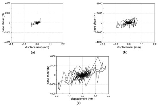
Figure 7.
Relationship between the bottom shear with the displacement in the second story in response to the El Centro waves: (a) 0.1g; (b) 0.2 g; (b) 0.3 g.
It can be seen in Table 6 that as the earthquake intensities increase, both the peak accelerations and displacements of the model increase significantly. For example, the peak displacement of the model responding to the El Centro waves (0.1 g) on the top floor is 0.61 m/s2, while the response under the El Centro wave (0.3 g) is 2.94 m/s2. Furthermore, the peak accelerations of the top floor are always larger than those of the second floor, reflecting the damage of the top floor may be more significant than that of the second floor. The influence of El Centro waves is consistently larger than that of the Qian’an waves. Figure 6 indicates that the peaks and valleys of acceleration responses under different waves with different intensities are mainly accumulated in the same time instants. It can be concluded, in Figure 7, that as the earthquake intensity rises, the relationship between bottom shear and the displacement in the second story is response to the El Centro waves significantly, which may be due to inner damages in the model.
5.2. Finite Element Simulation Results
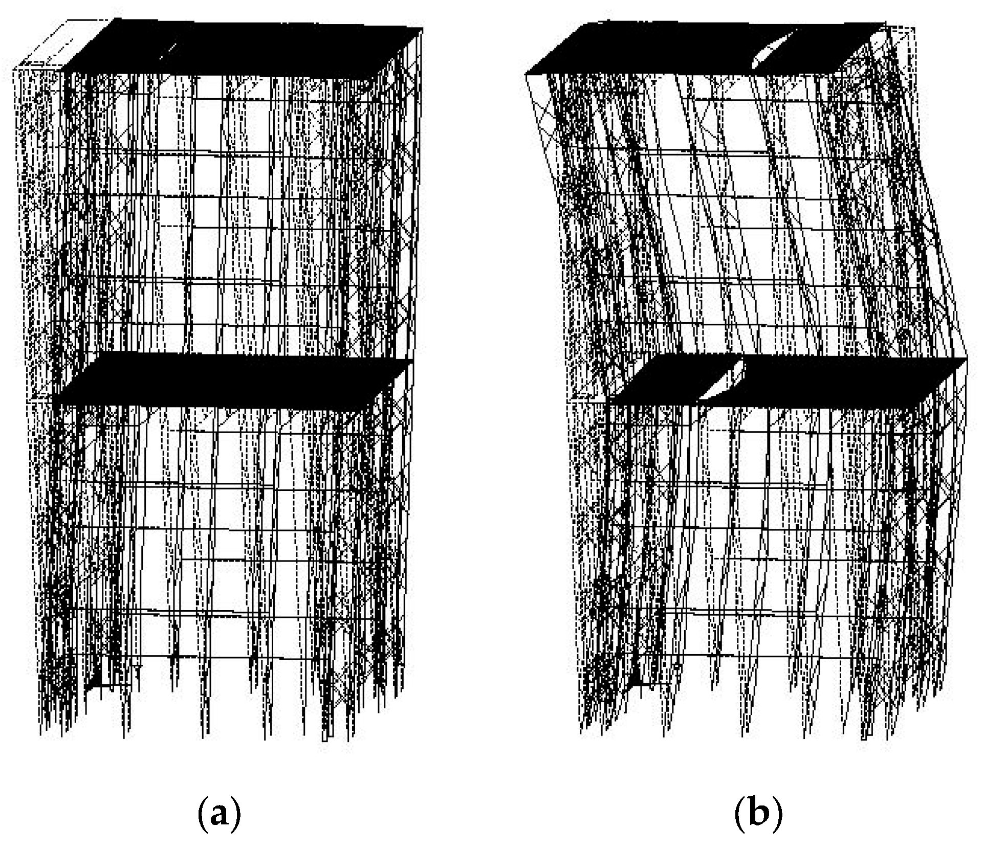
The first and second vibration modes are shown in Figure 8. The comparison between the dynamic characteristics in the experiment and the results in the FE simulation is shown in Table 7. It can be seen that the experimental and the FE simulation results are consistent with each other, indicating the FE simulation is reasonable. Therefore, the FE model can be used for further study.
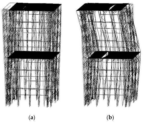
Figure 8.
Vibration modes of the FE model: (a) first mode; (b) second mode.
Table 7.
Dynamic characteristics of the model in the experiment and FE simulation.
The comparison between the peak displacement and acceleration responses in the experiment and the results in the FE simulation is shown in Table 8. The results of the FE simulation are consistent with results in the experiment. All the results indicate that as the earthquake intensity rises, the peak displacement and acceleration responses increase.
Table 8.
Peak displacement and acceleration responses of the model in the experiment and the FE simulation.
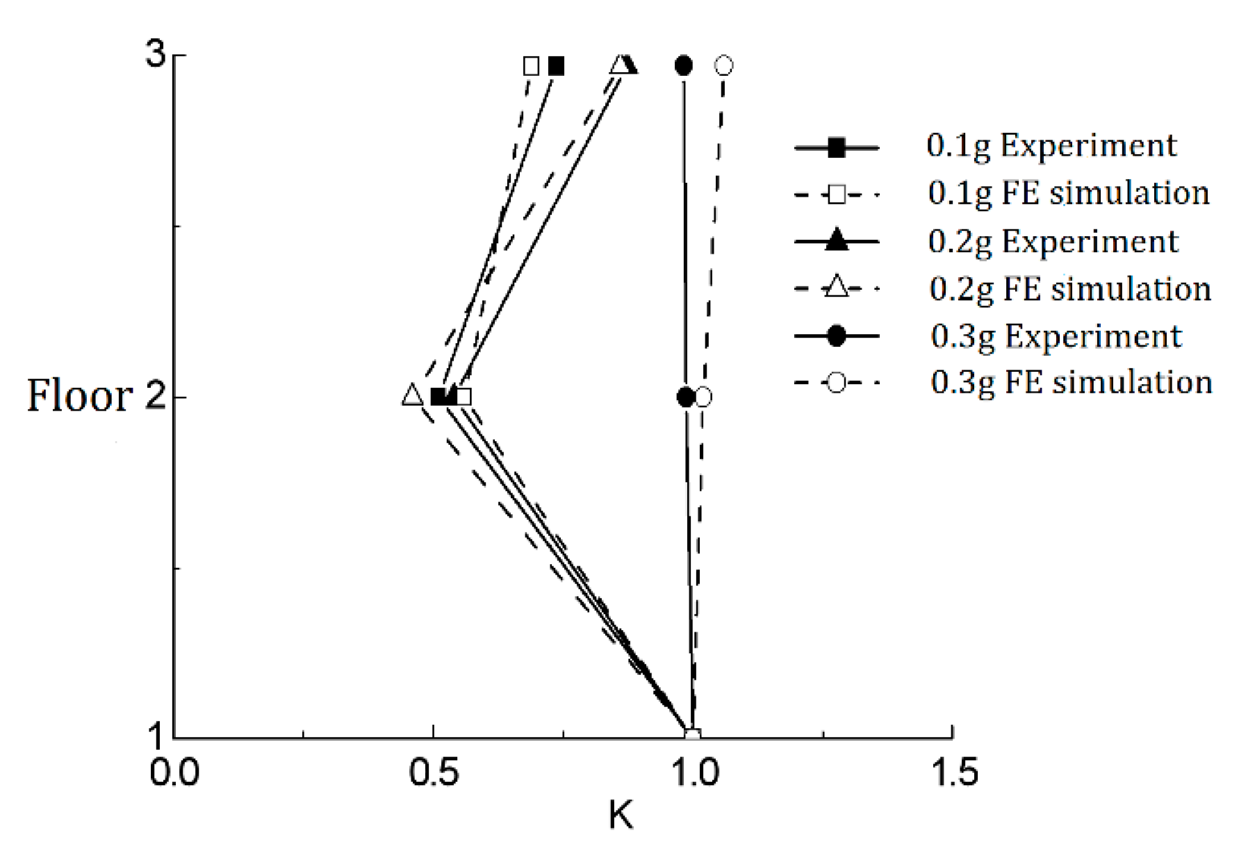
The acceleration amplification factor represents the ratio between the peak acceleration values of each story with the peak input accelerations at the shaking table. As shown in Figure 9, the acceleration amplification factors in the experiment and the FE simulation are similar. Therefore, it can be concluded that the acceleration responses are modest and indicate the satisfactory seismic performance of the model. The structure is an assembly structure that combines components with self-tapping screw connections. This type of connection is flexible and has a strong energy dissipation capacity, which may be greatly beneficial in providing earthquake resistance capacity.
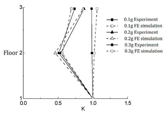
Figure 9.
Envelope of the acceleration amplification factor in response to El Centro waves.
5.3. Damage Detection Results
As mentioned before, the damage identification results can directly represent the property changes in the model structure. To further study the inner damage of the web steel structure under different earthquake intensities, the proposed damage detection method in Section 2 is adopted to identify the damage of the model. The study also includes comparisons between the AR model with additive noise and its adopted total least-squares (TLS) solution, as well as the classic AR model and least-squares (LS) solution.
The acceleration responses in the experiment excited by Gaussian white noise are used for detecting the damage levels and distributions of the model structure. The test model can be divided into two parts. The lower part is the first story, which is between the table surface and the second floor. The upper part is the second story, which is between the second floor and the top floor. The damage levels of the model structure are represented by the values of the detection indicator presented in Section 2. The structure is considered in healthy stage under the white noise excitation before the earthquake wave tests.
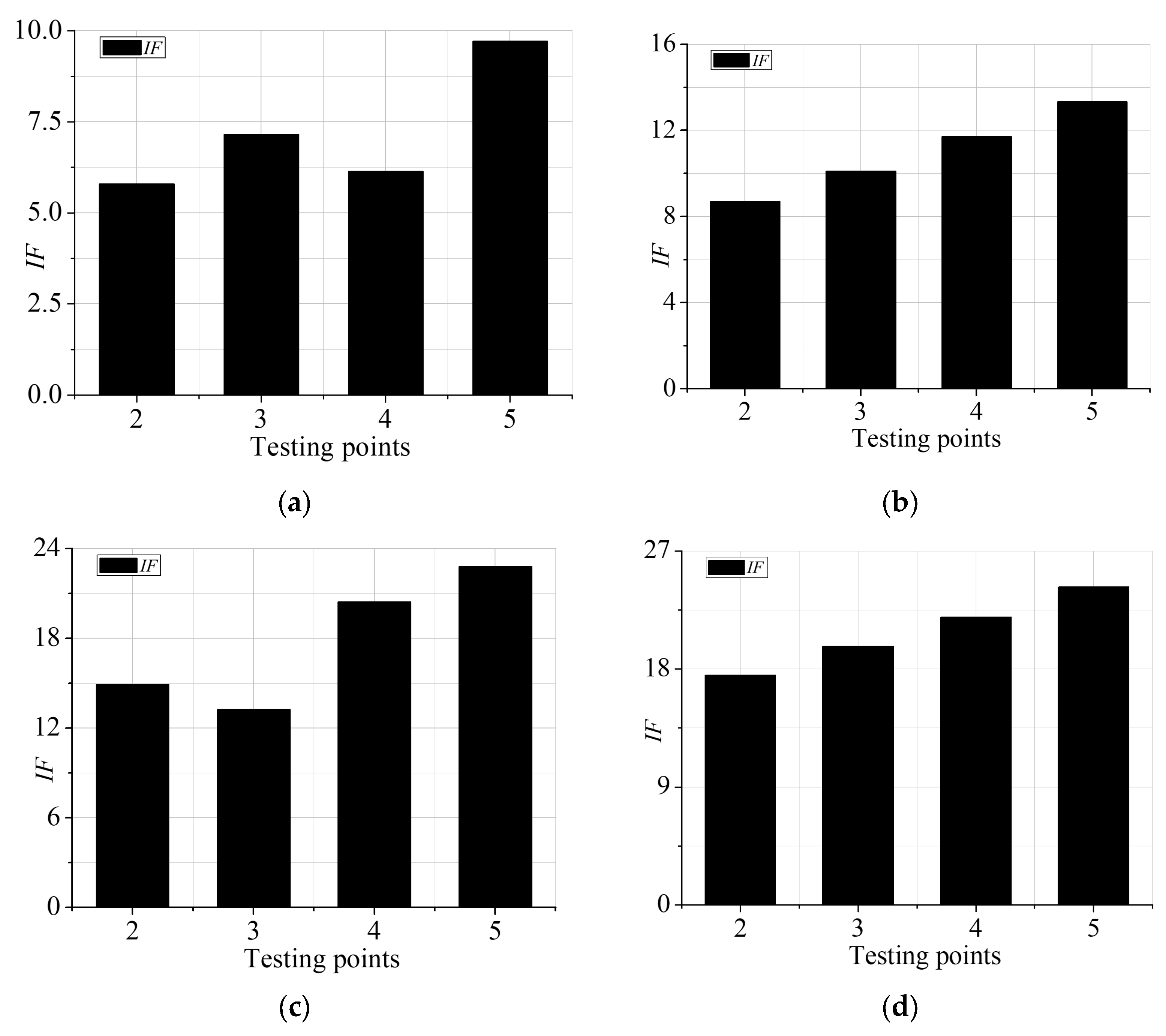
The IFs of each testing point under different intensities are shown in Figure 10. The results indicate that the intensity factors (IFs) increased as the seismic intensity rose in all testing points, indicating that damage to the structure increases with the earthquake level. Besides, the gaps between 0.27 g and 0.3 g are relatively small compared to those of other levels (except testing point 3, which may be due to some unknown mistakes). Which reflects that the damage identification method can be used to detect structural damage levels correctly.
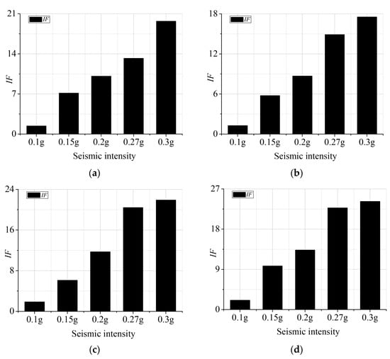
Figure 10.
IFs of different testing points: (a) point 1; (b) point 2; (c) point 3; (d) point 4.
The IFs of some accelerometer testing points under the same earthquake intensities are listed in Figure 11. Testing points 2 and 3 are on the second floor, and 4 and 5 are on the top floor. It can be concluded that the IFs of the first story are consistently larger than the IFs of the second story (except for seismic intensity of 0.2 g), indicating more damage occurs in the top part of the model structure. The damage to the top part increases more rapidly and easily as the seismic intensity rises. In addition, IF values of the two symmetrical testing points of the same floor are not the same, the eastern part (testing points 3 and 5) of the web structure model contains more damage, which shows that the west part of the model may have performed better. This may be due to construction errors. Moreover, all the IFs are relatively smaller (in comparison with the IFs in the mathematical simulation in Section 3), this indicates that the web steel model structure performs well under earthquake excitations.

Figure 11.
IFs of different testing points after the same intensities: (a) 0.15 g; (b) 0.2 g; (c) 0.27 g; (d) 0.3 g.
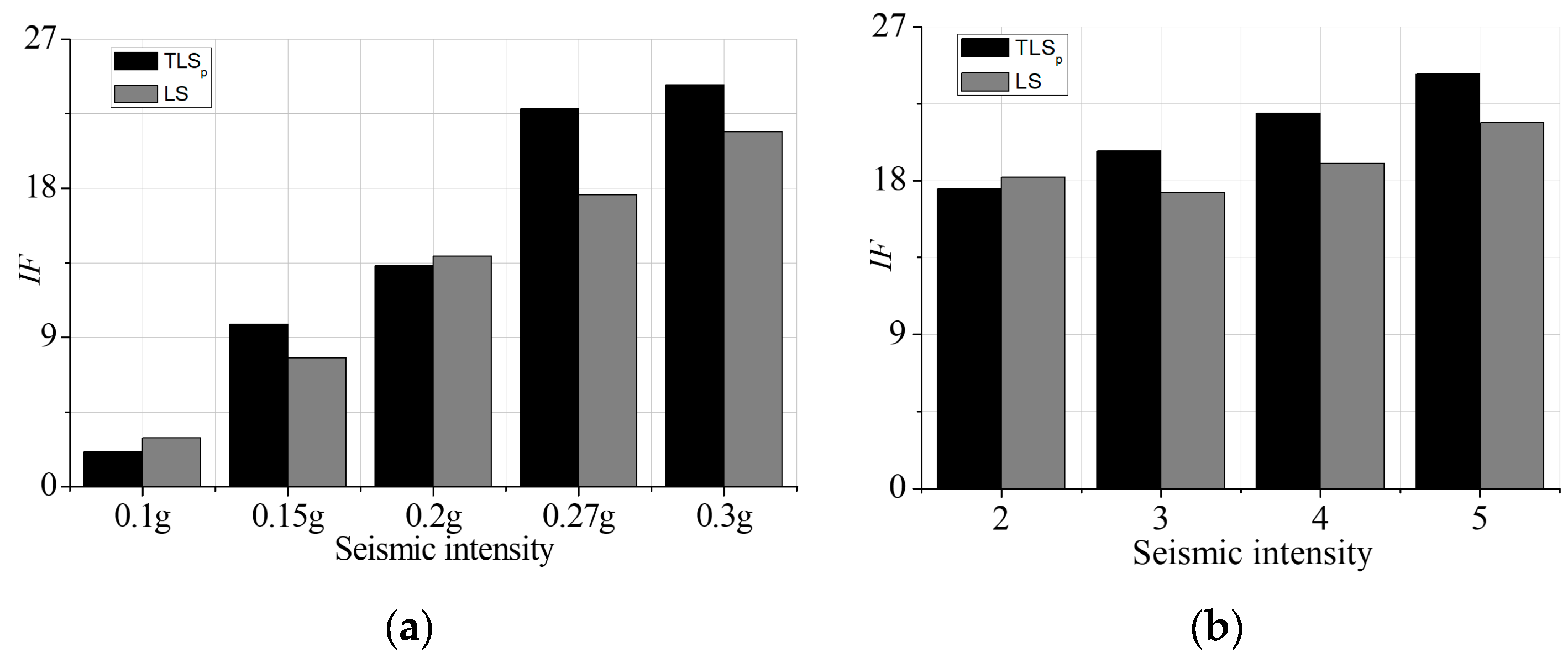
The differences between the results obtained by the detection method presented in Section 2 and the classical model and its LS solution are shown in Figure 12. It is clear that the IFs of the two methods are quantitatively different. For example, redarding testing point 5, the IF of the proposed method is larger than the IF of the LS solution at intensities of 0.27 g and 0.3 g, while being smaller at 0.1 g. Furthermore, the variations in IFs from the method are greater than that from the LS solution. It is argued that the differences attributed to the LS solution ignore possible errors in the designed matrix. Regarding the model of the proposed identification method TLSp, all the observation data in matrix A, which consisted of the acceleration time series output in this experiment, are considered as signals with noise. However, the AR model does not account for the presence of errors, despite the fact that these errors do exist during experimental operation, originating from manual operations, unstable sensor fixation, environmental noise, etc. Based on the TLSp model and its corresponding parameter estimation algorithm, a more accurate parameter solution should be obtained, thereby resulting in an IF that is closer to the true value. Hence the proposed damage identification method in this paper can be more suitable in practice use.
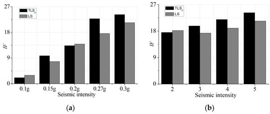
Figure 12.
Comparison between the damage detection results: (a) IFs of testing point 5; (b) IFs of seismic intensity 0.3 g.
To summarize, the experiment, FE simulation, and damage detection indicate that the web steel structure can perform well in response to seismic waves. As the earthquake intensity increases, the response values such as the acceleration and displacement of the model structure become large. Furthermore, by applying the proposed damage detection methods, it can be concluded that damage to the model rises with increases in earthquake intensity. However, none of the damage is significant, due to the good seismic performance of the web steel structure.
6. Conclusions
This paper presents a highly robust structural damage identification method that can maintain stability even in the presence of high levels of noise. The method overcomes the current limitations of AR-based damage identification, which is greatly affected by observation errors. This paper introduces a modified auto-regressive (AR) model that accounts for additive noise. Unlike traditional AR models, this modified model takes into consideration all the errors in observations. To solve the modified AR model, a total-least-squares (TLS) solution is adopted for the partial EIV model. In a mathematical simulation example, the solution of the modified AR model along with its TLS solution is compared to the classic AR model with the least-squares (LS) solution. The results demonstrate that the proposed method outperforms the traditional approach, even when dealing with high levels of noise. Additionally, an effective damage indicator is employed to measure the differences in AR parameters and quantify the extent of damage to a system. Finally, a shaking table test and the corresponding finite element (FE) simulation of a full-scale two-story web steel structure was conducted. The damage identification method proposed in this paper was also applied to the acceleration responses to further study the damage levels and distributions of the model structure under different earthquake conditions. It can be concluded from the results that the web steel structure studied in this paper performs well and that the damage incurred increases as the earthquake intensity increases. The damage detection method presented in this paper can detect both damage levels and distribution in the structure. This damage detection method may be effective for practical applications in civil engineering.
The proposed detection method shows promise in reducing identification errors compared to classical detection methods using the AR models and its LS solution. It exhibits relatively accurate results, even in conditions of high levels of noise. Furthermore, its performance with the web steel structure affected by earthquake waves can provide a valuable reference for further studies on similar structures.
However, structural information in a healthy state for comparison is always necessary when applying this method in practical engineering. This makes the identification impossible for structures that do not have stored healthy information. It also poses difficulties in installing sensors and monitoring signals for complex and hazardous structures. Future research could focus on the development and utilization of long-term stable embedded sensors for structures to be monitored. This would enable real-time monitoring of structural health based on the signals from these sensors combined with the damage identification method proposed in this study. Another thing to address is how to fix the sensors to structures to reduce the noise. These advancements would provide new avenues for tracking and identifying techniques in civil engineering.
Author Contributions
Methodology, Q.X. and D.Z.; Validation, Q.X.; Formal analysis, Q.X.; Investigation, J.L.; Resources, C.W.; Data curation, C.W.; Writing—original draft, D.Z.; Writing—review & editing, D.Z.; Project administration, J.L. and C.W. All authors have read and agreed to the published version of the manuscript.
Funding
The authors would like to express their gratitude to Natural Science Foundation of Jiangxi Province, China (No. 20232BAB214074) and the Central Non-Profit Scientific Research Fund for Institutes of China (No. CKSF 2021431/CL).
Data Availability Statement
All data supporting the findings of this study are available from the corresponding author upon reasonable request, but all personally identifiable information will be identified before transferal.
Conflicts of Interest
The authors declare no conflict of interest.
References
- Sarah, J.; Hejazi, F.; Rashid, R.S.; Ostovar, N. A Review of Dynamic Analysis in Frequency Domain for Structural Health Monitoring. IOP Conf. Series Earth Environ. Sci. 2019, 357, 012007. [Google Scholar] [CrossRef]
- Xiao, F.; Sun, H.; Mao, Y.; Chen, G.S. Damage identification of large-scale space truss structures based on stiffness separation method. Structures 2023, 53, 109–118. [Google Scholar] [CrossRef]
- Huynh, N.T.; Nguyen, T.V.; Nguyen, Q.M. Optimum Design for the Magnification Mechanisms Employing Fuzzy Logic-ANFIS. Comput. Mater. Contin. 2022, 12, 5961–5983. [Google Scholar]
- Huynh, N.T.; Nguyen, T.V.; Tam, N.T.; Nguyen, Q.M. Optimizing Magnification Ratio for the Flexible Hinge Displacement Amplifier Mechanism Design. In International Conference on Material, Machines and Methods for Sustainable Development MMMS 2020, Proceedings of the 2nd Annual International Conference on Material, Nha Trang, Vietnam, 12–15 November 2020; Springer: Cham, Switzerland, 2020; pp. 769–778. [Google Scholar]
- Ni, H.; Li, M.H.; Zuo, X. Review on Damage Identification and Diagnosis Research of Civil Engineering Structure. Adv. Mater. Res. 2014, 1006–1007, 34–37. [Google Scholar] [CrossRef]
- Wang, Y.; Gu, Y.; Liu, J. A domain-decomposition generalized finite difference method for stress analysis in three-dimensional composite materials. Appl. Math. Lett. 2020, 104, 106226. [Google Scholar] [CrossRef]
- Kabir, H.; Aghdam, M.M. A generalized 2D Bézier-based solution for stress analysis of notched epoxy resin plates reinforced with graphene nanoplatelets. Thin Walled Struct. 2021, 169, 108484. [Google Scholar] [CrossRef]
- Bert, C.W.; Malik, M. Differential quadrature: A powerful new technique for analysis of composite structures. Compos. Struct. 1997, 39, 179–189. [Google Scholar] [CrossRef]
- Ahn, S.; Park, G.; Yoon, H.; Han, J.-H.; Jung, J. Evaluation of Soil–Structure Interaction in Structure Models via Shaking Table Test. Sustainability 2021, 13, 4995. [Google Scholar] [CrossRef]
- Xiao, F.; Zhu, W.; Meng, X.; Chen, G.S. Parameter Identification of Frame Structures by considering Shear Deformation. Int. J. Distrib. Sens. Netw. 2023, 2023, 6631716. [Google Scholar] [CrossRef]
- Xiao, F.; Zhu, W.; Meng, X.; Chen, G.S. Parameter Identification of Structures with Different Connections Using Static Responses. Appl. Sci. 2022, 12, 5896. [Google Scholar] [CrossRef]
- Kopsaftopoulos, F.P.; Fassois, S.D. Vibration based health monitoring for a lightweight truss structure: Experimental assessment of several statistical time series methods (conference paper). Mech. Syst. Signal Process. 2010, 24, 1977–1997. [Google Scholar] [CrossRef]
- He, J.; Chen, J.; Ren, X.; Li, J. A shake table test study of reinforced concrete shear wall model structures exhibiting strong non-linear behaviors. Eng. Struct. 2020, 212, 110481. [Google Scholar] [CrossRef]
- Moaveni, B.; He, X.; Conte, J.P.; Restrepo, J.I. Damage identification study of a seven-story full-scale building slice tested on the UCSD-NEES shake table. Struct. Saf. 2010, 32, 347–356. [Google Scholar] [CrossRef]
- Li, S.; Wu, C.; Kong, F. Shaking Table Model Test and Seismic Performance Analysis of a High-Rise RC Shear Wall Structure. Shock. Vib. 2019, 2019, 6189873. [Google Scholar] [CrossRef]
- Wu, C.; Li, S.; Zhang, Y. Structural Damage Identification Based on AR Model with Additive Noises Using an Improved TLS Solution. Sensors 2019, 19, 4341. [Google Scholar] [CrossRef] [PubMed]
- Hakim SJ, S.; Mokhatar, S.; Shahidan, S.; Chik, T.; Jaini, Z.; Ghafar, N.A.; Kamarudin, A. An ensemble neural network for damage identification in steel girder bridge structure using vibration data. Civ. Eng. Archit. 2021, 9, 523–532. [Google Scholar] [CrossRef]
- Wickramasinghe, W.R.; Thambiratnam, D.P.; Chan, T.H.T.; Nguyen, T. Vibration characteristics and damage detection in a suspension bridge. J. Sound Vib. 2016, 375, 254–274. [Google Scholar] [CrossRef]
- Morita, K.; Teshigawara, M.; Hamamoto, T. Detection and estimation of damage to steel frames through shaking table tests. Struct. Control. Health Monit. 2005, 12, 357–380. [Google Scholar] [CrossRef]
- Chen, W. Auto-Regressive Model Estimation Theory and Its Application in Deformation Monitoring Data Processing. Ph.D. Thesis, Wuhan University, Wuhan, China, 2013. [Google Scholar]
- Binder, M.D.; Hirokawa, N.; Windhorst, U. Auto-Regressive Model; Springer: Berlin/Heidelberg, Germany, 2008. [Google Scholar]
- Bernagozzi, G.; Achilli, A.; Betti, R.; Diotallevi, P.P.; Landi, L.; Quqa, S.; Tronci, E.M. On the use of multivariate autoregressive models for vibration-based damage detection and localization. Smart Struct. Syst. 2021, 27, 335–350. [Google Scholar]
- Zheng, W.X. A least-squares based method for autoregressive signals in the presence of noise. IEEE Trans. Circuits Syst. Part II Analog. Digit. Signal Process. 1999, 46, 81–85. [Google Scholar] [CrossRef]
- Diversi, R.; Guidorzi, R.; Soverini, U. Identification of autoregressive models in the presence of additive noise. Int. J. Adapt. Control. Signal Process. 2008, 22, 465–481. [Google Scholar] [CrossRef]
- Zeng, W. Effect of the Random Design Matrix on Adjustment of an EIV Model and Its Reliability Theory. Ph.D. Thesis, Wuhan University, Wuhan, China, 2013. [Google Scholar]
- Diversi, R.; Soverini, U.; Guidorzi, R. A new estimation approach for AR models in presence of noise. IFAC Proc. Vol. 2005, 38, 160–165. [Google Scholar] [CrossRef]
- Esfandiari, M.; Vorobyov, S.A.; Karimi, M. New estimation methods for autoregressive process in the presence of white observation noise. Signal Process. 2020, 171, 107480. [Google Scholar] [CrossRef]
- Guidorzi, R.; Diversi, R. Structural health monitoring application of errors-in-variables identification. In Proceedings of the 2013 21st Mediterranean Conference on Control and Automatino (MED), Platanias, Greece, 25–28 June 2013; Volume 2013, pp. 1098–1103. [Google Scholar]
- Mahboub, V.; Amiri-Simkooei, A.; Sharifi, M. Iteratively reweighted total least squares: A robust estimation in errors-invariables models. Surv. Rev. 2013, 45, 92–99. [Google Scholar] [CrossRef]
- Datteo, A.; Busca, G.; Quattromani, G.; Cigada, A. On the use of AR models for SHM: A global sensitivity and uncertainty analysis framework. Reliab. Eng. Syst. Saf. 2018, 170, 99–115. [Google Scholar] [CrossRef]
- Xu, P.; Liu, J.; Shi, C. Total least squares adjustment in partial errors-in-variables models: Algorithm and statistical analysis. J. Geodesy 2012, 86, 661–675. [Google Scholar] [CrossRef]
- Xu, P. The effect of errors-in-variables on variance component estimation. J. Geodesy 2016, 90, 681–701. [Google Scholar] [CrossRef]
- Khorshidi, S.; Karimi, M. Finite Sample FPE and AIC Criteria for Autoregressive Model Order Selection Using Same-Realization Predictions. EURASIP J. Adv. Signal Process. 2010, 2009, 475147. [Google Scholar] [CrossRef]
- Code for Seismic Design of Buildings (GB50011-2010); Ministry of Housing and Urban Rural Development of the People’s Republic of China; China Architecture & Building Press: Beijing, China, 2010.


Disclaimer/Publisher’s Note: The statements, opinions and data contained in all publications are solely those of the individual author(s) and contributor(s) and not of MDPI and/or the editor(s). MDPI and/or the editor(s) disclaim responsibility for any injury to people or property resulting from any ideas, methods, instructions or products referred to in the content. |
© 2023 by the authors. Licensee MDPI, Basel, Switzerland. This article is an open access article distributed under the terms and conditions of the Creative Commons Attribution (CC BY) license (https://creativecommons.org/licenses/by/4.0/).