Validation of One Predominant Frequency Presence in Seismic Ground Displacement by Means of Deformation Response Spectra

Abstract

There are very few results in the literature on spectral content of seismic ground displacement; nonetheless, these results are singular as most of the spectral content is limited to a very narrow low frequency band, contrary to ground acceleration. These few spectral characterizations have been obtained, expectedly, by means of power spectral or Fourier analyses of ground displacement records, only. As these records are not as reliable as ground acceleration records, the existence of a clear predominant frequency in ground displacement warrants confirmation through a different procedure. We propose a corroboration method of this highly narrow-band characteristic that is based on the more dependable acceleration signal, rather than on the same ground displacement record that is the subject of study. Specifically, displacement response spectra are analyzed (which rely on acceleration records) to verify previously observed neat predominant frequencies in ground displacement, which is a novelty.

1. Introduction

In earthquake engineering, acceleration records are the standard and established input signal; therefore, displacement (and velocity) seismological records have not received as much attention in structural dynamics. There are reasons for this: (1) the common seismic equations of motion have the acceleration of the ground (times an inertial constant of course) as force on the right-hand side, (2) what is mostly measured by seismic instruments is acceleration (because accelerographs are more robust), and (3) the displacement record is hardly obtained directly, but is (mostly) instead obtained from integrating the acceleration record. Nevertheless, this is not a simple numerical calculus algorithm but a very complex process. As a matter of fact, there is a whole research field called seismic record processing [1] because signal noise is a major problem, which implies that correction and filtering procedures are part of these complex processes. The common seismic equation of motion referred to above, in its simplest form, is $m\ddot{x}+c\dot{x}+kx=-m\ddot{s}$, where x is the structure’s relative displacement, s is the ground displacement, and m, c and k are the mass, stiffness and damping coefficient of the simple structural model, respectively.

However, there are also many reasons to give more attention to ground displacement. The displacement record is important in the analysis of long-span structures, long pipes and tunnels [2], and in the control of base-isolated structures [3,4], which have a large base displacement (LBD) problem under earthquakes [5]. More generally, in earthquake engineering there has lately been some displacement in interest, from force-based design to displacement-based design (DBD) [6]. It has recently been asserted, e.g., for the LBD problem in isolated buildings, that if structural displacement is the problem, the focus regarding excitation should be on ground displacement rather than ground acceleration [5]. Finally, it is pointed out that it is not an absolute fact that the forcing function (equation’s right-hand side) must be ground acceleration; in fact, that input term can also be written in terms of ground velocity and displacement or a combination thereof [4,7].

As introduced above, there is difficulty in conducting analyses with ground displacement signals, as this seismic record is not as reliable as the corresponding or original acceleration record. Most seismic instruments measure acceleration, so to obtain ground displacement, the analyst has to doubly integrate the measured record, and it is in the resulting displacement where the noise involved and the unknown baseline are very problematic. Indeed, the computed displacements may be wild or quite unphysical [1]. Nevertheless, newer digital recorders are superior to the old analog ones for this important matter [1,8,9]; therefore, research can be carried out with more confidence on the displacement and velocity signals as time passes or technology advances.

An example of this change over time is the study of spectral content of seismic ground displacement, which was originally studied using mostly signals from analog recorders [4,10]. A concern at the time was the low-frequency noise affecting the results observed, which were a highly narrow-band characteristic in the displacement records at around 0.15 Hz. Later, a similar study was carried out being the differences or novelties (1) a broader area of the world, and more importantly (2) a full set of digital records [11]. It is noted that these two characteristics are related, as regions in the developing world have implemented seismic networks and stations later, compared to Japan, California and Taiwan. As a favorable result, the capacity or possibility of measuring strong motion close to the epicenter and with digital recorders is much greater in the former regions. More important were the confirming results, which corroborated that horizontal ground displacement is a narrow-band process, with the dominant frequencies in a very limited and defined low-frequency range, roughly between 0.05 and 0.15 Hz.

Digital records are in fact superior to analog ones; in particular, noise at long periods is greatly reduced, which implies that significant data at ever lower frequencies can be obtained. Indeed, the low-cut frequency in the filtering process reached 0.02 Hz in analysis of the 1999 Hector mine earthquake [12], which was one of the first three events in the world that were recorded predominantly digitally [1]. Moreover, a mean value low-cut frequency of 0.03 Hz was found for a significant (magnitude larger than 7) set of earthquakes in Latin America from the most recent decade [11]. Nonetheless, digital records are not perfect and processing is still necessary, not mainly because of noise now but for the acceleration baseline, which still needs adjustment [12]. Thus, although we have more dependable displacement records than 20 years ago, any results associated with seismic ground displacement are still received with some level of reservation. Therefore, such results may need to be proven by a second or even third means. This is what is carried out in this study; the research gap encountered is that there was no reliable or direct confirmation of the fact that seismic ground displacement has a clear and neat predominant frequency close to 0.1 Hz, which was demonstrated first by power spectral density (PSD) analyses [10,11]. More lately, the result has been corroborated indirectly by solving an actual earthquake engineering problem, the LBD, by controlling the isolator displacement by the inerter [5]. This solution or good time-domain results on the control of the base relative displacement would not have been possible if the ground displacement did not have a prominent peak close to 0.10 Hz, as that is the main hypothesis in the frequency-domain design or optimization procedure. It is worth noting that a predominant frequency of 0.10 Hz for ground displacement, was obtained independently by Tian and Yang [13].

In this study, the existence of one dominant frequency in ground displacement is verified by studying displacement response spectra; this corroboration through this methodology is novel. This corroboration procedure has a main advantage, in that it is based on ground acceleration data, which are more reliable than displacement data, even in the case of the newer digital records. Therefore, any reservation about the ground displacement spectral results obtained by direct PSD analyses should be reduced if there is a match with the results of the proposed study. The idea is that a dominant or critical frequency (maximum power) is recovered from the previous PSD results [10,11], then resonance is searched for on the independent (of displacement record) deformation response spectra for the very same seismic records. If a peak at or near the critical frequency is also observed in the response spectrum, this would be an argument in favor of the conclusion that seismic ground displacement has a clear or narrow predominant band, contrary to ground acceleration. More importantly, it would be argued that this spectral band is indeed centered at those critical frequencies, which were limited to the 0.05–0.15 Hz range in most cases, except for the rare liquefaction records [10,11].

Finally, it is important to mention that past attempts to define predominant frequencies of earthquakes, which were based on acceleration (either of the ground or as response spectra), had difficulties in obtaining clear results or reasonable standard deviations [14,15]. In fact, the “scatter” in results were (in the authors’ words) “excessively large” [15]. The novel idea here, and in previous work regarding the displacement record, is that clearer seismic predominant frequencies are possible if one studies the most basic motion quantity, displacement, either directly as the input displacement or as the displacement response.

2. Method

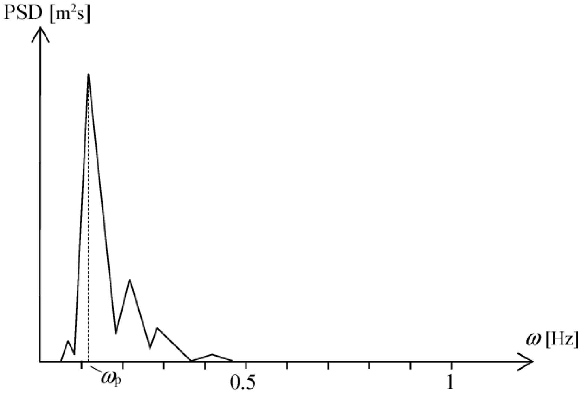
It has been previously demonstrated that Fourier or power spectra of horizontal ground displacement have the general form shown in Figure 1 [10,11,13]; although most of this graphic is pictorial, the frequency axis is exact to a certain degree, as there is clear similarity to what is observed in the actual power spectrum results in the literature. These highly narrow-band results have been validated by a solution to an actual earthquake engineering problem [5] where the standard ground acceleration is used as input in the simulations, which is independent of the displacement signal that one is analyzing. Another type of corroboration of the existence of clear and neat predominant frequencies in ground displacement, which is also independent of that record, is presented herein. The proposed validation is based on an analysis of displacement response spectra, as explained next. It is stressed that this response spectrum has not been studied as much as the acceleration spectrum.

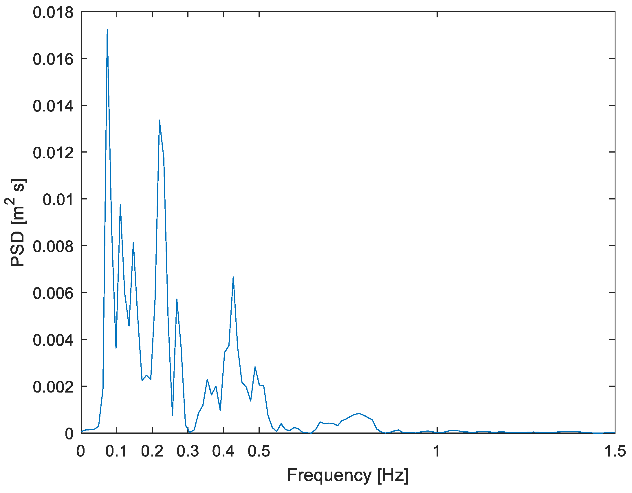
First, one predominant frequency is retrieved from the calculated or available PSD (Fourier spectra) of ground displacement. This input predominant frequency ω_p (Figure 1) is defined as the frequency corresponding to the peak value of the PSD [16]; it is noted that these terms (central frequency is another spectral parameter e.g.) have thus far been used almost exclusively for ground acceleration spectra in Earthquake Engineering.

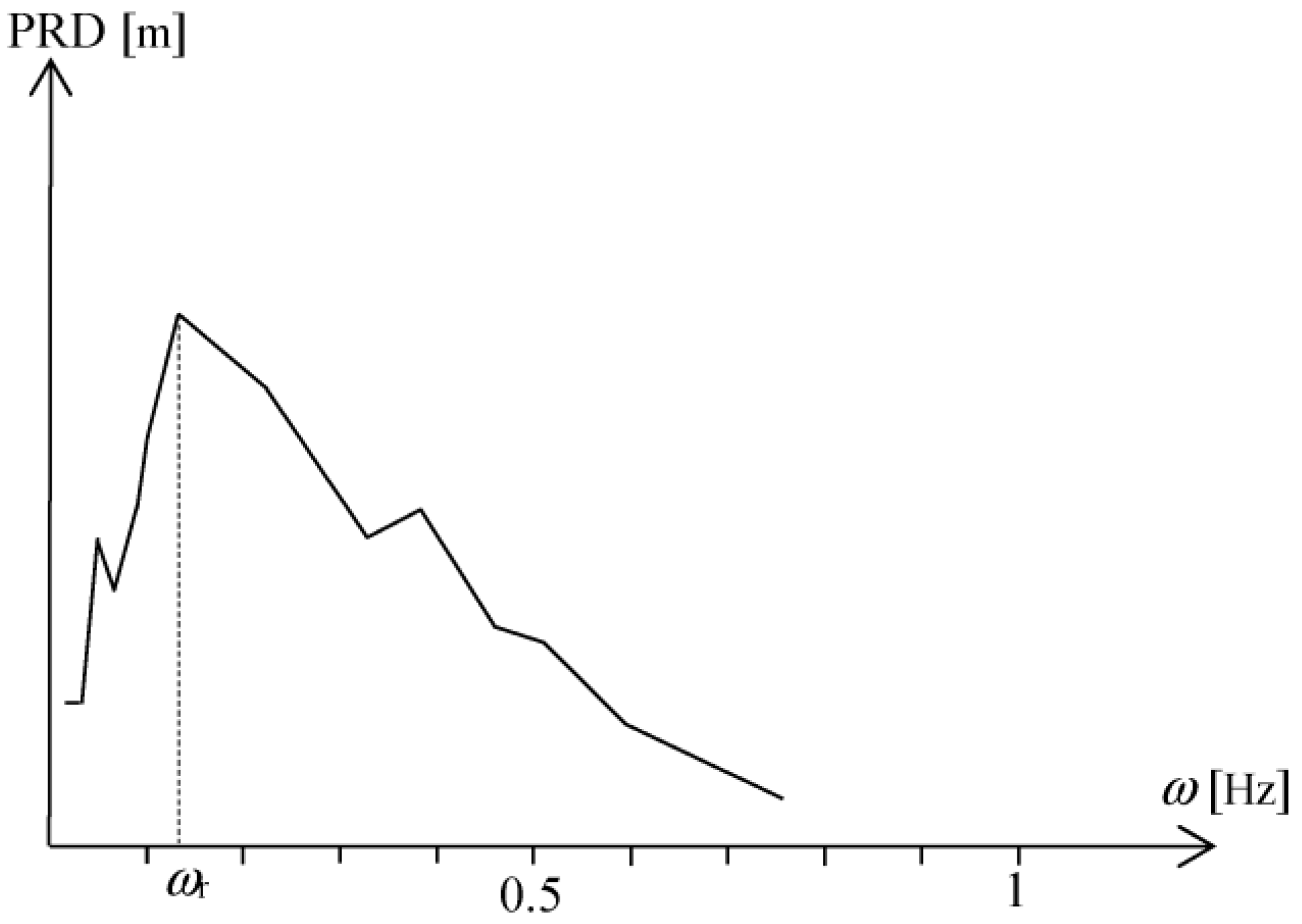
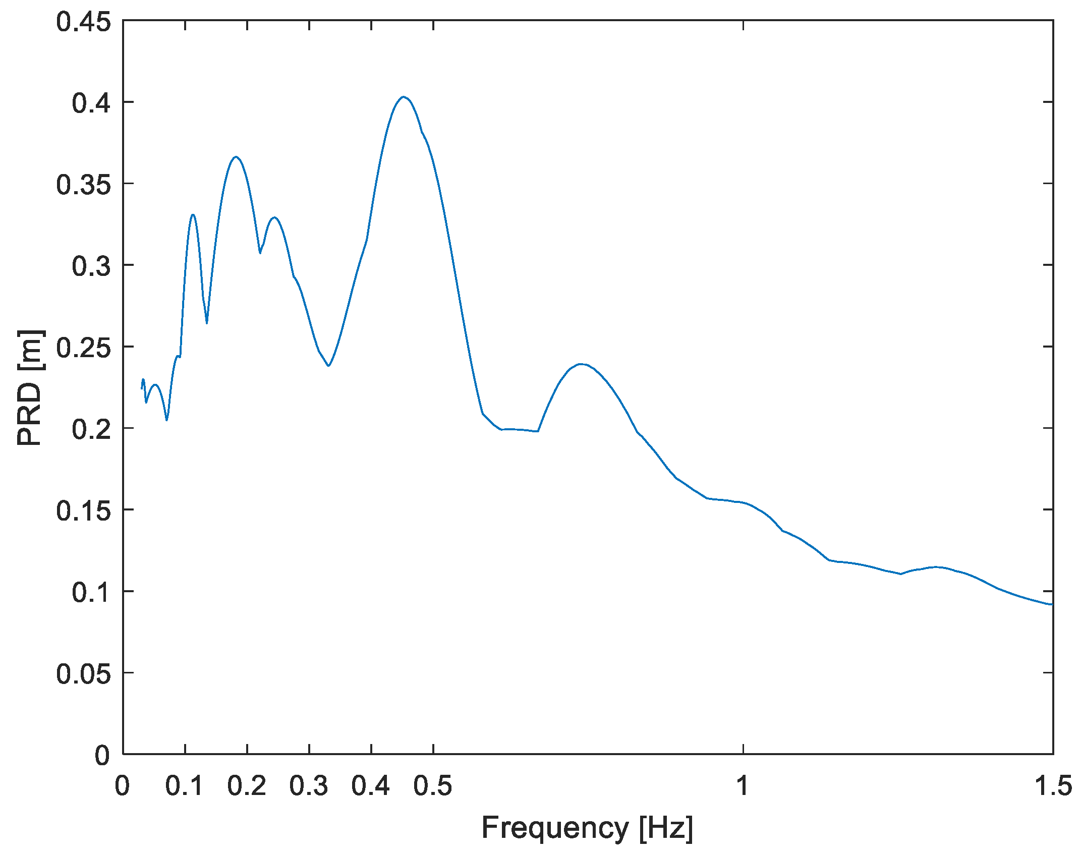
Secondly, in the displacement response spectrum, not only corresponding to the same seism but also to same station and component, resonance or dominant frequencies will be looked for. The hypothesis of this investigation, based on the theoretical development starting in next paragraph, is that not only a clear resonance, or output predominant frequency ω_r (Figure 2), will be observed but, more importantly, this will be near to the input displacement PSD predominant frequency, or that ω_r ≈ ω_p. More clearly, or in graphic terms, we will be observing what is shown in Figure 2. This plot is peak response displacement, PRD, against natural frequency, or simply displacement response spectrum. The comment or slight difference is that response spectra are more commonly published against a natural period and with logarithmic scale. Similar as above or for the input, we formally define ω_r following the common definitions for acceleration, as the structural natural frequency (period) at which the maximum spectral displacement occurs in the response spectrum [15] for 10% damping.

It is emphasized that here we are dealing with two different types of spectra, one for the excitation and the other for the response. Before doing the match analysis between both, a more theoretical basis for the study and its hypothesis are given in terms of basic and random vibrations concepts. In fact, it has to be explained why it is necessary to study the displacement response spectrum instead of the ordinary acceleration spectrum when looking for or confirming predominant frequencies. Additionally, which displacement response should be studied—the absolute displacement spectrum or the common deformation (relative displacement) one?

This study verifies predominant frequencies in input (ground) displacement through response (output) spectra; as there is no interest in the ordinary ground acceleration, it is natural to choose the structural displacement as the quantity of interest on the response side, because it is the structural response quantity most directly related to the seismic excitation signal of interest. This direct and mathematical relationship between ground and structural displacements will be shown at this stage. Before, it is noted that there are two response displacements, the absolute and the relative one (note that there are no options on the input side: ground displacement is always absolute). From Mechanical Vibrations, both direct output–input relationships are very clear through either the transmissibility [4,17] or the relative transmissibility [5,11] concepts, which mathematically relate the structural and input displacement amplitudes as [17]

$$T=\frac{X}{S}=\frac{\sqrt{1+{\left(2\zeta r\right)}^2}}{\sqrt{{\left(1-r^2\right)}^2+{\left(2\zeta r\right)}^2}}$$

(1)

where X and S are the absolute and the ground displacement amplitudes, respectively; and as [11]

$$T_r=\frac{X_r}{S}=\frac{r^2}{\sqrt{{\left(1-r^2\right)}^2+{\left(2\zeta r\right)}^2}}$$

(2)

where X_r is the relative displacement or structural deformation amplitude, r is the frequency ratio and ζ is the damping factor. It can be argued that these simple input–output displacement ratios, somewhat overlooked in Earthquake Engineering, are valid only for harmonic excitation; however, it can be proven by means of Random Vibrations that the transmissibility idea is a more general concept, as shown next by employing a simple one-degree-of-freedom system under stochastic or seismic load.

It can be shown through random vibration theory that the mean square value of the structure’s absolute displacement, α, can be expressed in terms of ground displacement; in this regard, an original result is

$$\alpha =2\underset{0}{\overset{\infty }{\int }}{\left|H\right|}^2\left(c^2{\omega }^2+k^2\right) S_{ss}d\omega$$

(3)

where H is the frequency response function, k and c are the stiffness and damping coefficient, and S_ss is the ground displacement power spectral density. Thus, seismic structural displacement (absolute) can be written absolutely in terms of the input displacement PSD, considering that the other factor in the integrand is defined by the structural system. Moreover, it can be demonstrated without much difficulty that this factor is the transmissibility, squared because we work with mean squares in random vibrations, or

$${\left|H\right|}^2\left(c^2{\omega }^2+k^2\right)=\frac{1+{\left(2\zeta r\right)}^2}{{\left(1-r^2\right)}^2+{\left(2\zeta r\right)}^2}=T^2$$

(4)

In the relative case, the conclusion is similar; the mean square value of the relative displacement can be written in this case as

$${\alpha }_r=2\underset{0}{\overset{\infty }{\int }}{\left|H_r\right|}^2 S_{\ddot{s}\ddot{s}}d\omega =2\underset{0}{\overset{\infty }{\int }}{\left|H_r\right|}^2{\omega }^4 S_{ss}d\omega$$

(5)

where $S_{\ddot{s}\ddot{s}}$ is the ground acceleration PSD. Again, it can be stated that the seismic structural deformation is directly and mathematically related to the random ground displacement; nonetheless, even more interesting is the fact that this stochastic relationship is through the transmissibility, T_r in this case, or that

$${\left|H_r\right|}^2{\omega }^4=\frac{r^4}{{\left(1-r^2\right)}^2+{\left(2\zeta r\right)}^2}=T_r^2$$

(6)

which can also be demonstrated without much effort. Therefore, it has been shown that if one is studying ground displacement by means of seismic response analysis, displacement is or well may be the structural response to be focused on, because the relationship is neat and clear. The statement may, or may not, appear obvious, but it required some demonstration because acceleration has, through the decades, been the usual variable in Earthquake Engineering and traditional force-based design in both the excitation and the response [18]. The question remains as to which of the two displacement responses to choose in our proposed method. The relative displacement response spectrum is chosen simply because it is more related to Earthquake Engineering, as it is deformation, or strain.

Because the hypothesis (of earlier in this Section) that ω_r ≈ ω_p has been given a theoretical basis by proving that there is a very clear and direct relationship between ground displacement and structural deformation, we now define the important measure of this research:

$$\delta =\frac{\left|{\omega }_{\mathrm{r}}-{\omega }_{\mathrm{p}}\right|}{{\omega }_{\mathrm{r}}}$$

(7)

which is a relative difference between the predominant frequency of the seismic input, as displacement and the natural frequency of the structure that resonates (in displacement) under the same record. This resonant frequency ω_r is the output predominant frequency. Of course, this difference δ is not expected to be zero, because (1) ω_p and ω_r are the simplest of spectral parameters as they do not say anything about the shape of the spectrum or secondary dominant components, (2) power spectrum and resonance are both stationary concepts but earthquakes last usually no longer than 50 s or are actually nonstationary random processes, and (3) the processed ground displacement signal may not be correct. However, it is expected that δ be near zero or less than 0.15 (15%) in most cases because there is already an important level of certainty in that seismic ground displacement can be modelled as highly narrowband. In general, a 10% difference or less is not expected or will be surprising because of the 3 important reasons above. The term highly narrowband is used because it is observed that 0–1 Hz, the whole ω-axis in Figure 1 (or in the actual and subsequent figures) is already a narrow range, considering that a common range of the ω-axis in power spectra of ground acceleration is 0–15 Hz [14].

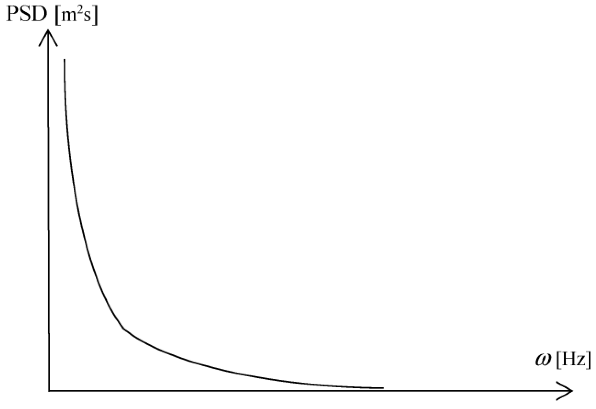
Finally, before the results are presented, an important comment is in order regarding the necessity of more study on the ground displacement spectral content. It can be argued that because the ground displacement PSD is equal to the ground acceleration PSD over ω⁴ [19] (ω in rad/s), there is no need for more validation of the existence of a narrow predominant band in ground displacement; however, such an argument would only prove part of the spectral picture, or would show only what is presented in Figure 3 (theoretically, e.g., using a Kanai–Tajimi acceleration PSD), which is a narrow-banded, or compressed against ω = 0, displacement PSD, but not the narrowbandness observed in practice (Figure 1 or subsequent real PSD plots), which is not centered at ω = 0 at all [10,11]. In fact, the concentration in this work is more on these unique and predominant ω_p ≠ 0 than on the narrow-band characteristic.

3. Results

As explained, first, the predominant frequencies will be retrieved from power spectra of ground displacement. More than twenty events with magnitudes larger than 6.5, mainly from the Americas (from Chile to California) but including two from outside this region, will be considered. In fact, displacement PSD (as Figure 1) for most of these earthquakes are available for the closest to epicenter stations from previous works [10,11]. Subsequently, we will obtain the corresponding deformation response spectra, as Figure 2, as thoroughly explained in the previous section. It is stressed that the response spectrum must be computed and plotted for right the same strong-motion record for which power spectrum is also calculated or available, the same event is not sufficient, not even the same station.

Thus, the predominant frequency for those input displacement signals have been obtained and are shown in column 3 of

Table 1. Input predominant (ω_p) and response resonant natural frequencies (ω_r).

Earthquake	Station and Component	ωp [Hz]	ωr [Hz]	δ
Kern County (1952)	Taft, 111°	0.110	0.111	0.01
San Fernando (1971)	Pachoima Dam, 164°	0.146	0.166	0.12
Imperial Valley (1979)	Calexico, 315°	0.122	0.130	0.06
Coalinga (1983)	Pleasant Valley, 45°	0.122	0.093	0.31
Superstition H. (1987)	Imperial Wildlife, 0°	0.305	0.290	0.05
Loma Prieta (1989)	Corralitos, 90°	0.146	0.167	0.13
Petrolia (1992)	Cape Mendocino, 0°	0.159	0.167	0.05
Landers (1992)	Joshua Tree, 90°	0.122	0.107	0.14
Northridge (1994)	Northridge Church, 0°	0.073	0.452	0.84
Eureka (1994)	Cape Mendocino, 0°	0.098	0.086	0.14
Chi Chi (1999)	Taichung 78, 90°	0.085	0.076	0.12
Hector Mine (1999)	Amboy, 360°	0.195	0.168	0.16
Haiti (2010)	Presa Sabenta, 360°	0.046	0.090	0.49
Maule (2010)	Constitución, T	0.275	0.255	0.08
Sierra Cucapá (2010)	Bond’s Corner, 90°	0.134	0.115	0.17
Coquimbo (2015)	Pedregal, 90°	0.064	0.067	0.04
Ecuador (2016)	Otavalo, 90°	0.060	0.059	0.02
Kaikoura (2016)	Te Mara, 332°	0.226	0.195	0.16
Chiloé (2016)	Espejo Luna, 360°	0.038	0.040	0.05
Valparaíso (2017)	Torpederas, 90°	0.110	0.125	0.12
Puebla (2017)	UNAM, 90°	0.183	0.176	0.04

, ω_p. Some of those published power spectrum plots were against circular frequency (rad/s); for the results here, all will be in Hertz; thus, response spectra will also be constructed against frequency rather than period (seconds), which is more common in civil engineering. In fact, we calculated or reconstructed most input PSD plots (e.g., Figures 4, 6, 8, 10 and 12).

3.1. Deformation Response Spectra

The corresponding (same station and component) relative displacement response spectra are computed and plotted, for ζ = 0.1. Here, predominant or resonant frequencies ω_r will be searched for in these output spectra and compared through Equation (7) to the input predominant frequency. For brevity, and because the interest is only in the maxima, we present only five output spectra plots as examples, alongside their corresponding input spectra. Specifically, full plots are presented for the best two results (δ = 0.009, Kern Co.; δ = 0.017, Ecuador), the worst two results (δ = 49%, Haiti; δ = 84%, Northridge), and the mean result, which is Hector Mine (δ = 0.161 or 16%), an event with the δ very close to the mean value: 0.157. For all the cases, the resonant natural frequency is shown in column 4 of Table 1, and the relative difference (Equation (7)) in column 5. The five selected output spectra are shown in Figures 5, 7, 9, 11 and 13, while the corresponding input spectra are shown in Figures 4, 6, 8, 10 and 12. It is noted that for some events on the US west coast, deformation response spectra may be available directly through CESMD (strongmotioncenter.org); however, for the long-period range (T > 5), the ordinates are for periods separated by 0.5 s, which imply a very low resolution in this low-frequency range where the interest is. On the input side, note also that most ground displacement PSD considered here have been published [10,11], but some of those original plots were against circular frequency.

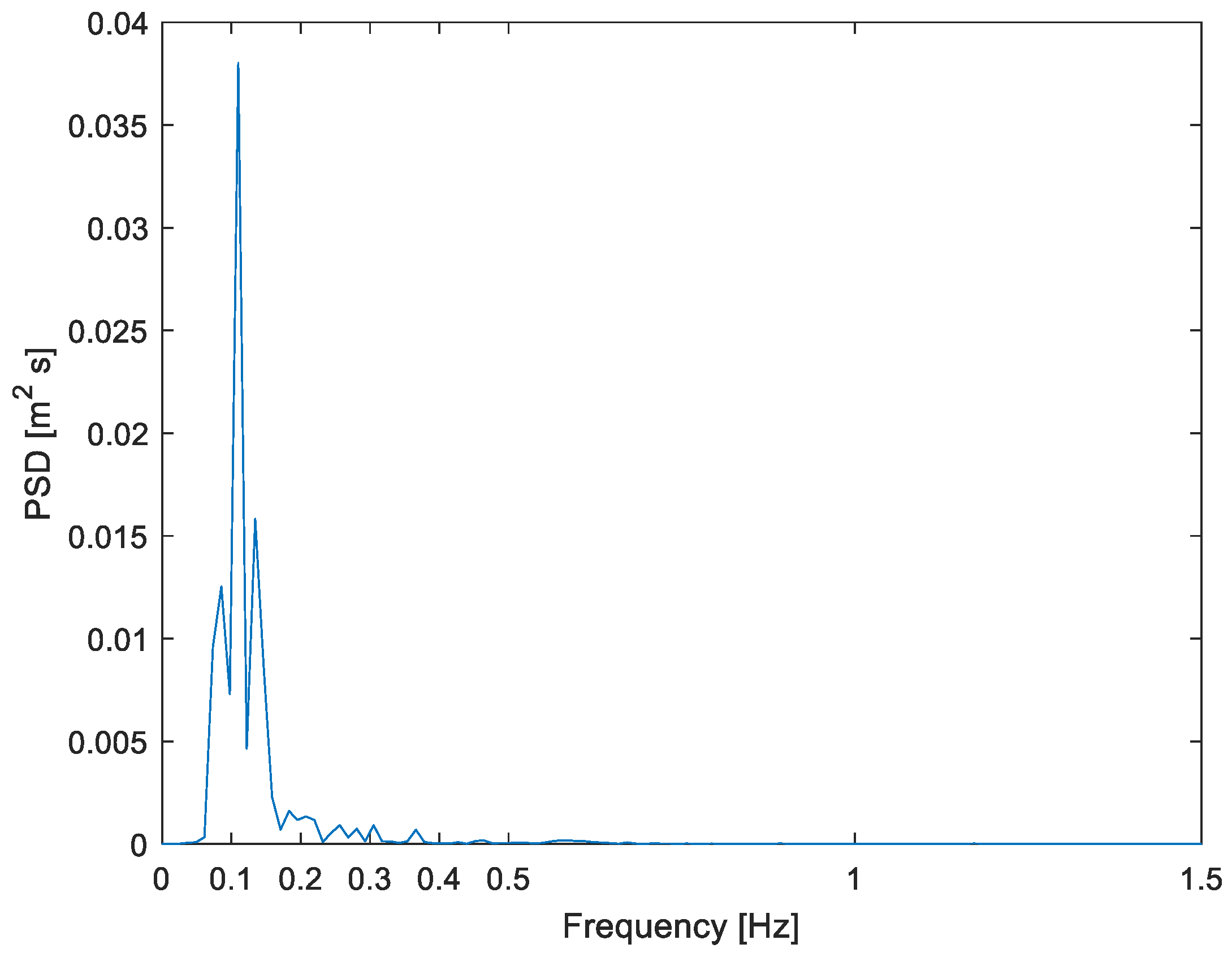
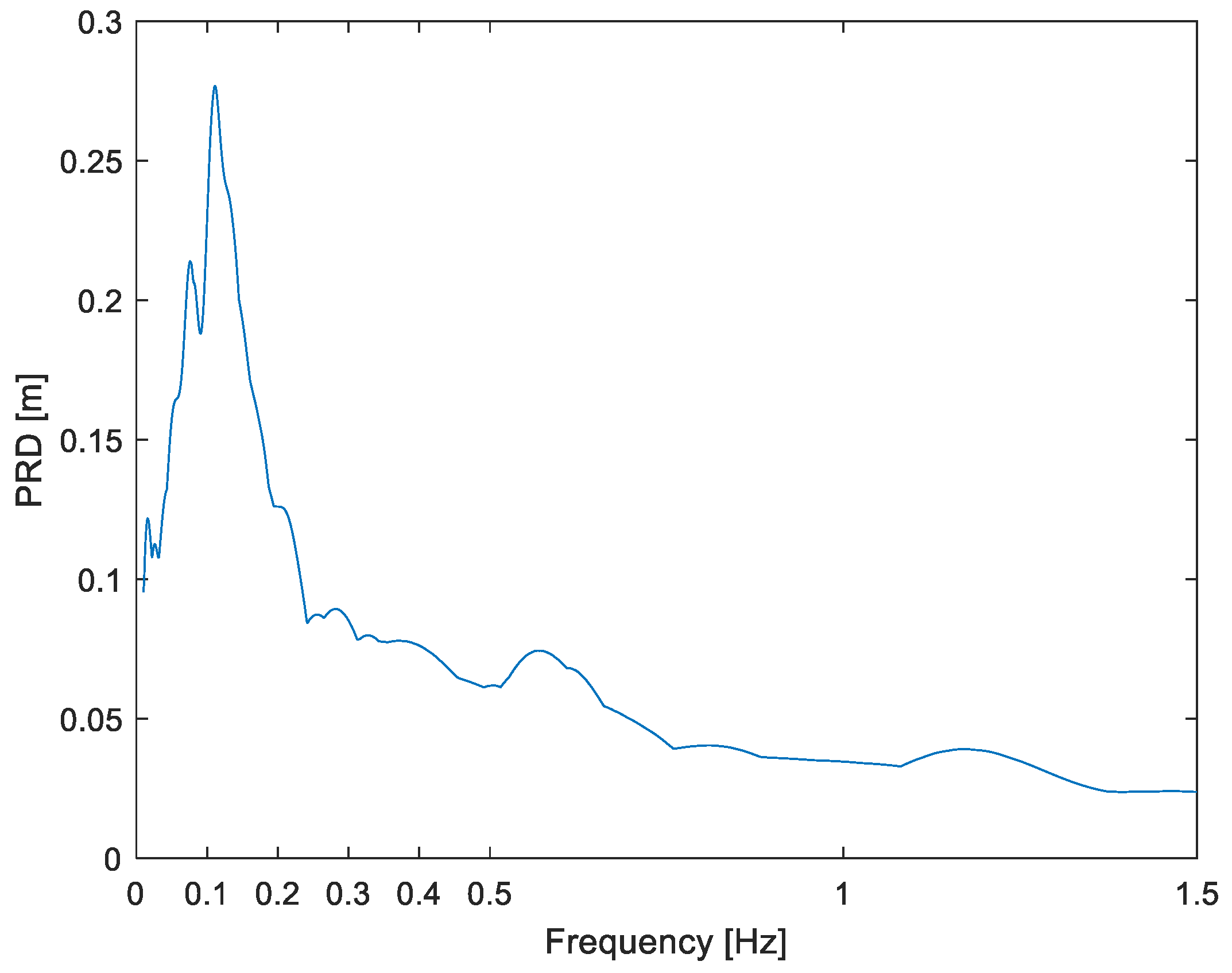
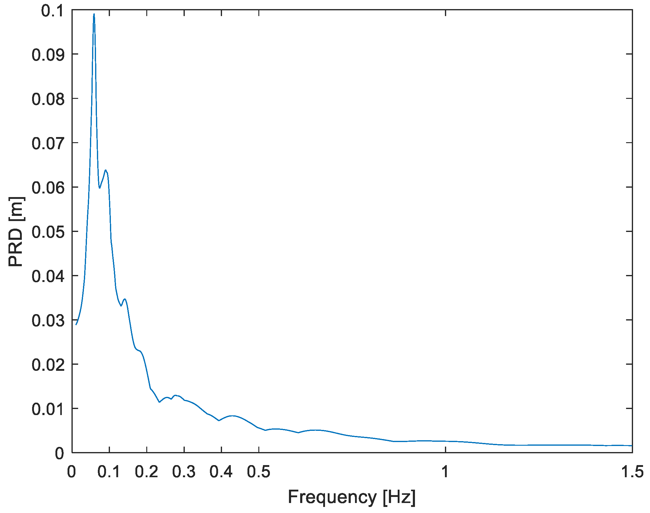
The results are, indeed, more than excellent in the first two of the selected cases; for the Kern Co. event, there is a very clear input predominant frequency at 0.110 Hz (Figure 4) and a clear output predominant frequency at 0.111 Hz (Figure 5) for a relative difference of almost zero or just 0.9%, which means an almost perfect match. In fact, Kern Co. at Taft is our best result. For the second event (Ecuador), critical frequencies are 0.060 (input, Figure 6) and 0.059 Hz (output, Figure 7) for δ = 1.7%. In Figure 6, the highly narrow-band characteristic of ground displacement can be well appreciated; note that the full plot domain is of a mere 1.5 Hz but still a strong concentration of energy is observed, at 0.06 Hz. In these two cases, the difference is not only well below the expected value (0.15; Method section) but even well below 5%.

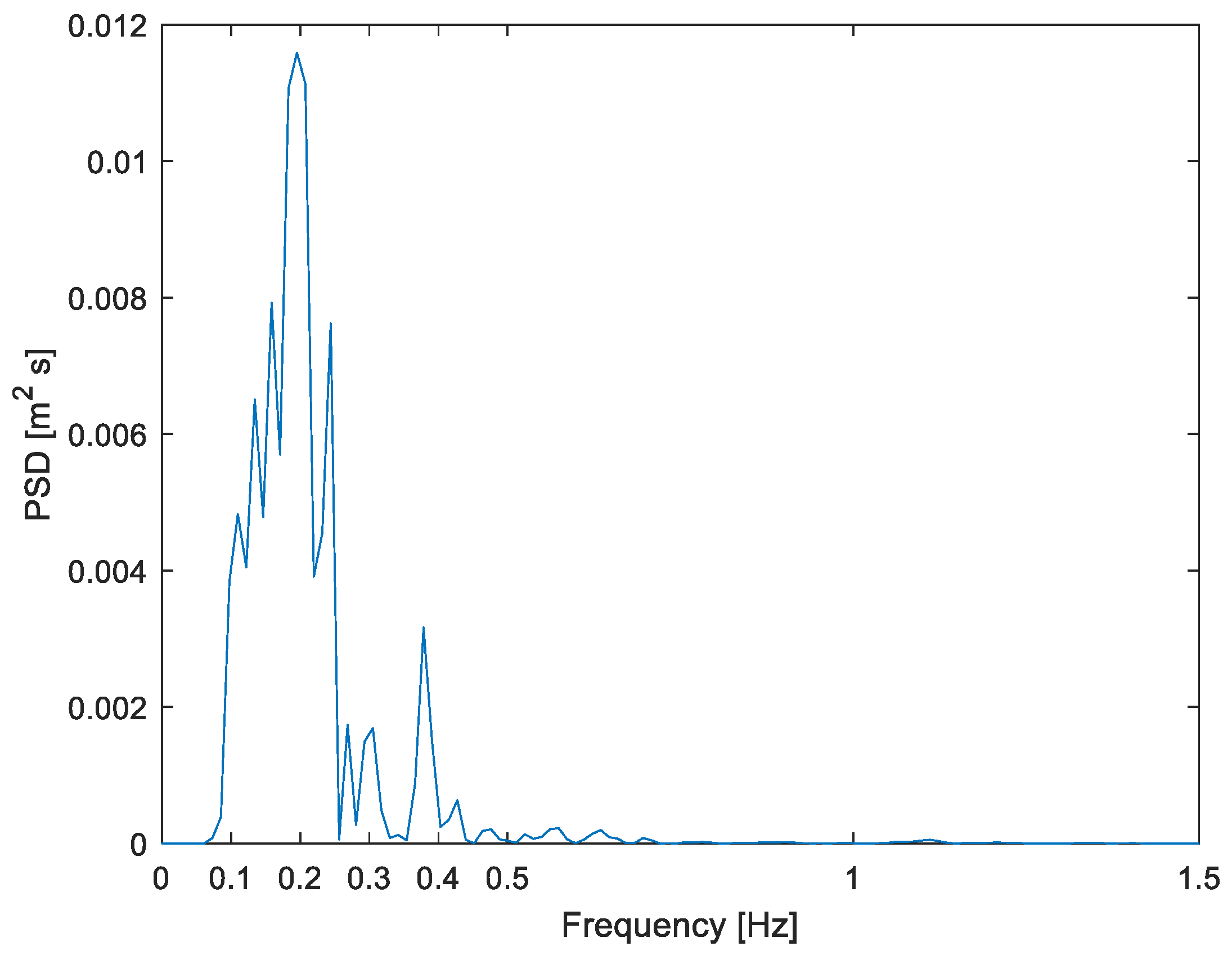
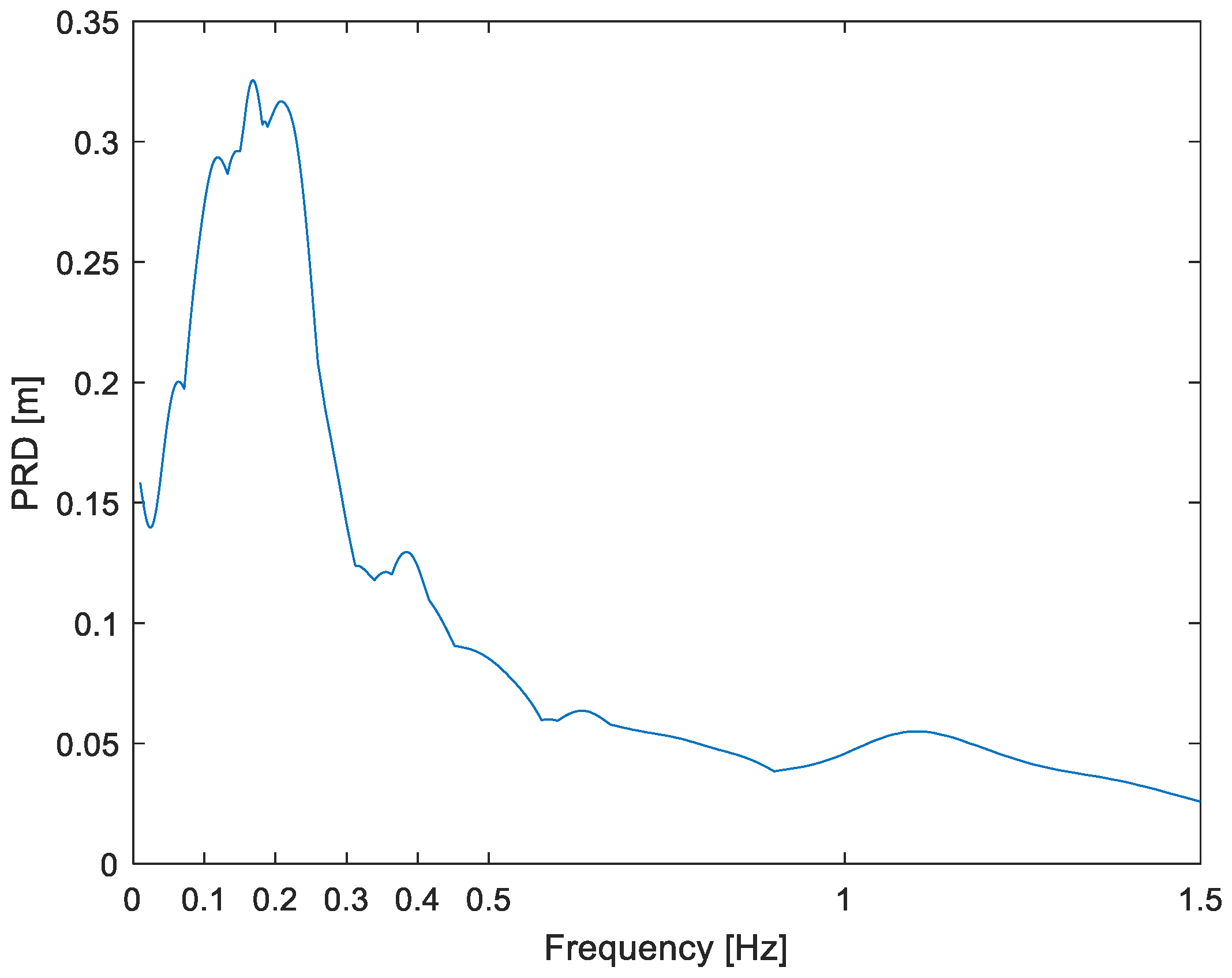
In the Hector Mine event (middle case), even though the narrow-banded nature of ground displacement can still be seen in Figure 8 (where also the entire ω-axis is just 0–1.5 Hz), it is not as neat as in the PSD of Figure 6. In this case, the dominant frequencies are more distributed, with significant energy between 0.10 and 0.25 Hz. This band can also be observed in the response spectrum (Figure 9). As a result, in practice it would be very difficult for the two critical frequencies to be ω_r ≈ ω_p; however, δ = 16% is still a respectable result.

Now, let us see the two results that are not good; for the Haiti seism there are actually two dominant input frequencies, at 0.05 and 0.09 Hz (Figure 10), and the resonant frequency is 0.09 Hz (Figure 11). The bad δ result (0.49) was obtained, of course, with the first dominant frequency because it is predominant; in fact, this 49% result is irremovable from Table 1 or the Method must be respected. However, it is worth pointing out that with the second dominant frequency, δ would be 2%, which would be a very good result or spectral match. More formally, the processed ground displacement, of which PSD is calculated, may not represent very well the true displacement in the case of Haiti. It must be stressed that both seismic record processing and power spectrum calculation are not at all absolute or unique procedures. The situation is more problematic in the Northridge case (δ = 0.84) where the resonant ω_r = 0.45 Hz does not have a match until the fifth input dominant frequency, which can be read as 0.43 Hz (Figure 12 and Figure 13). These two issues, associated with the two worst results, will be discussed more in the next Section, but this type of problem is associated to reason three in the second-to-last paragraph of the Methods section: the processed ground displacement record may not be fully correct.

3.2. Overall Analysis of Results and Remarkability of the Set of Seismic Records

An overall conclusion drawn from Table 1 is that for 71% of the records considered, the relative difference δ is below the 0.15 expected or hypothesized in the Methods section; moreover, for a third of the cases δ ≤ 0.05. These relative differences, in general, are considered to be very good results; nonetheless, all results will be discussed more in the next section. It is noted that the Superstition H., Northridge and Maule records are liquefaction situations, which is the reason for consistent predominant frequencies above 0.25 Hz.

Finally, it is emphasized that the records are not arbitrary. First, the earthquakes were all above 6.5 in magnitude. Second, the chosen stations were the closest to the epicenter, and the horizontal component with the largest peak displacement was selected in each case. That is, we are dealing with a notable set of earthquakes, mainly from the whole of the Americas (from California to Chile) but including two higher than 7.5 from the rest of the world. The common characteristic of the set is the huge magnitude; in fact, the soil conditions of the stations are very diverse, from Alluvium (Taft e.g.,) to Rock (Pacoima Dam), from Dense Soil (Corralitos) to Deposits (Espejo Luna). Indeed, another important conclusion may be that site geology is not a critical parameter when studying predominant frequencies if the analysis is based on displacement rather than on common acceleration, because we are observing a clear narrow band of predominant frequencies that seems independent of site condition; however, this would require further and future research considering this parameter in more detail.

4. Discussion

For a clear majority or more than 70% of the records considered, the difference (relative) between the input displacement predominant frequency (ω_p) and the deformation response resonant frequency (ω_r) is below 0.15. These are expected and confirming results (Section 2), which are excellent. Indeed, for 43% of the cases, the difference is below 0.1 (10%). These positive results are validations of (1) the existence of one clear predominant frequency in ground displacement, (2) the narrowbandness of these seismic records, and (3) which these predominant frequencies are. Therefore, it can be concluded that the limited band of the PSD centered at ~0.1 Hz, obtained previously and similar to Figure 1 [10,11], has been confirmed. In fact, the mean value of δ is 15.7%, which is quite close to the 15% expected. The advantage of this method is stressed: it is based on ground acceleration data, which are more reliable than the displacement signal. In other words, we do not rely solely on the same record whose characteristics we are investigating.

Nevertheless, there are events as Haiti and Northridge here for which the relative difference is larger than 40%. However, there is an explanation for this difference; for example, in the case of the Haiti record, the second dominant frequency of the input is the one observed in the output as the predominant one. In fact, if one uses the second dominant frequency of the ground displacement, δ becomes less than 5%. Simply, in these two cases, the processed ground displacement, of which power spectrum is calculated, do not represent well the true displacement; in this regard, it must be emphasized that both seismic signal processing and PSD calculations are not infallible, absolute or unique procedures. Moreover, it is also noted that liquefaction occurred at or near the Northridge Church seismic station [20].

It can be argued that the displacement response spectrum plots do not show a very clear resonant frequency, or that the spectral predominance is not as neat as on the input side (PSD). However, two facts must be pointed out. First, resonance is a steady-state concept that would require theoretically infinite time, whereas an earthquake is quite a transient phenomenon; moreover, it should be recalled [19] that the PSD concept carries a square or is a squared function (a measure of energy actually). Therefore, predominance is heightened in a power spectrum, as compared to a simple Fourier spectrum or other spectra as a seismic response one.

It is important to highlight that past attempts to define predominant frequencies of earthquakes had solid difficulties in obtaining clear results or reasonable standard deviations [14,15]. Indeed, the “scatter” in the results were “excessively large” [15]. It is considered in this work that the problem lies in that the previous concentration has been on acceleration (either of the ground or as response spectra). The novel idea is that clearer seismic predominant frequencies are possible if one studies the most basic motion quantity: displacement, either directly as the input displacement, or as the displacement response. The findings of this research support and justify that idea because clear predominant frequencies have been observed in deformation response spectra.

5. Conclusions

Considering the discussion above on the reason for the few negative results, which is seismic signal processing, the positive conclusion is a corroboration of one predominant frequency existence in ground displacement, and which these frequencies are. It can be stated that the new or matching δ results here are a third proof of the results on spectral content of seismic displacement, because a previous confirmation by other means than Fourier analysis has been quite recently presented: a successful structural control of isolated buildings through inerter [5]; that is, the passive control proposed therein was successful because ground displacement has a predominant frequency near 0.10 Hz.

A limitation of this study is the fact that soil conditions and fault distance were not studied formally; therefore, future work should be attempting to define a seismic predominant frequency, considering both near-field (only) records and site geology. In fact, we are carrying out that research at this point in time. Another work proposed for the future can be to establish a bandwidth parameter to better define the narrow-band characteristics found when analyzing displacement.