Abstract
Major disasters and losses would be caused by the galloping of transmission lines. The basis for studying the galloping mechanism of transmission lines is to analyze the aerodynamic characteristics of iced conductors. The wind tunnel test is a traditional way to obtain the aerodynamic coefficients of an iced transmission line under wind load. Due to the high cost and long duration of wind tunnel tests, an experimental method based on machine learning to predict aerodynamic coefficients is proposed. Here, the steady and unsteady aerodynamic coefficients of an iced conductor under different parameters were obtained by wind tunnel test, and then the aerodynamic coefficients of the iced conductor under different parameters were predicted by machine learning. The aerodynamic coefficients of each iced conductor varied with the angle of wind attack by the wind tunnel test. The Den Hartog and Nigol coefficients determined based on the aerodynamic coefficients obtained by machine learning and wind tunnel test are in agreement. The results show the feasibility of the machine learning prediction method.
1. Introduction
China has actively created significant power transmission projects in recent years, and the country has also successfully reduced its electricity demand. However, during construction, transmission lines will cross some areas with dangerous terrain and complex environmental climates. Transmission lines are covered in ice all year round due to low temperatures, but especially in the winter. When wind in the horizontal direction acts on an iced conductor, it will cause aerodynamic loads, which will lead to the occurrence of galloping. Analyzing the aerodynamic coefficients of the iced conductor is the premise for studying the galloping mechanism of transmission lines. Many wind tunnel tests and numerical simulations of UHV transmission lines have been carried out in China [1,2,3]. The study of vibrations brought on by galloping and other flows has also recently received increased interest—in particular, the investigation of vortex-induced vibration (VIV) of flexible structures and self-excited galloping/flutter control of a civil structure [4,5].
Currently, research on the aerodynamic coefficients of iced conductors relies on an expensive and time-consuming method called the wind tunnel test. Additionally, the influence of outside circumstances can result in erroneous test findings. With the rapid development of machine learning research, neural network methods in machine learning have been widely used in many fields. Meng et al. [6] proposed a wavelet neural network with an enhanced particle swarm optimization algorithm to precisely describe the aerodynamic properties of an airplane. Wang et al. [7] used the RBF network to build an aerodynamic model of an aircraft and obtained the aerodynamic parameters of the aircraft. Raeesi et al. [8] proposed a quasi-steady analysis method, and the effect of unsteady/turbulent winds on the aerodynamic behavior of inclined cables was then studied. Ignatyev et al. [9] modeled unsteady aerodynamic properties based on the neural network method. The dynamic characteristics in a wide range of angles of attack were studied. Wang et al. [10] put forward a power system gallop early warning algorithm based on SVM and AdaBoost classification algorithms. Lee et al. [11] validated a prediction model of galloping accidents using a logistic regression model and used the corresponding AUC results of the ROC curve to assess the discriminant level of the estimated model. Ma et al. [12] considered the galloping of elliptical cylinders at critical Reynolds numbers under normal winds and evaluated the quasi-steady hypothesis when predicting these vibrations. Winter et al. [13] combined the regression local linear neural fuzzy model (NFM) with a multi-level perceptron (MLP) neural network to establish a recognition method for nonlinear systems. Li et al. [14], based on the principles of deep learning, proposed an unsteady atmospheric dynamics model for large-scale training data and sample spaces. Wang et al. [15] proposed a fuzzy neural network based on radial bases. It effectively addressed the limitation of the number of various input variables. Chen et al. [16], based on a convolutional neural network (CNN), proposed a graphical prediction method of airfoil multi-aerodynamic coefficients. Jaffar et al. [17] performed a comparative study of the damping coefficient characteristics of different workshops based on two independent neural network models, support vector regression, polynomial regression, and linear regression. Mannini et al. [18] proposed a nonlinear wake oscillator model that predicts the unstable galloping of slender structures in large-scale turbulence. Mou et al. [19] obtained aerodynamic coefficients through numerical simulation and used the extra trees algorithm to establish a prediction model of the aerodynamic coefficients of iced quad-bundle conductors. Then, it could predict and analyze the characteristics of the iced conductor galloping. Rykaczewski et al. [20], based on an artificial neural network, modeled the aerodynamic characteristics of a striped wing miniature aircraft.
However, predictive research on the aerodynamic coefficients of iced conductors under the impact of various conditions is lacking. Unsteady aerodynamic coefficient projections have not yet been seen. Therefore, the aerodynamic coefficients of iced conductors were first measured in a wind tunnel. Then, a model was created by using machine learning. The aerodynamic parameters of iced conductors under different parameters were predicted, and the results of the wind tunnel test were compared. The results show that the aerodynamic coefficients obtained by the two methods are the same with the variation in the angle of wind attack. The Den Hartog and Nigol coefficients derived by the two different methods of calculating aerodynamic coefficients are quite similar to the change curve with the angle of wind attack. The issue of time-consuming and expensive wind tunnel tests has been successfully resolved, which is helpful for managing and preventing transmission line galloping.
2. Wind Tunnel Test
2.1. Test Model
Wind-driven wet snow on transmission lines in winter can accumulate on the windward side, forming hard deposits with sharp edges. The final asymmetric shape of the ice may cause galloping. China has conducted extensive research on ice shape in recent years. Yu et al. [21] experimentally studied the dependence of the size and shape of ice on the duration of the ice and some structural properties. Xu et al. [22] studied the aerodynamics of circular cylinders with and without ice accretion through wind tunnel tests. Crescent ice and sector ice are two common forms of ice covering transmission lines and are the most likely to occur. The focus of this study is iced conductors in crescent and sector shapes. The aerodynamic coefficients were ascertained by the test. The cross-sectional model of the crescent-shaped ice conductor is shown in Figure 1a. The cross-sectional model of the sector-shaped ice conductor is shown in Figure 1b.
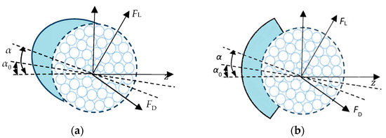
Figure 1.
Crescent-shaped and sector-shaped ice cross-sections.
The artificial ice model was constructed of wood with a density of 836.81 kg/m3, which is comparable to real ice. The test diameter of the model was 1:1 smaller than that of the actual conductor model, which had a diameter of 30 mm. The cross-section of the iced conductor is shown in Figure 2. The transmission conductor is shown in Figure 3.
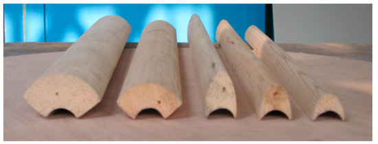
Figure 2.
Cross-section of the iced conductor.
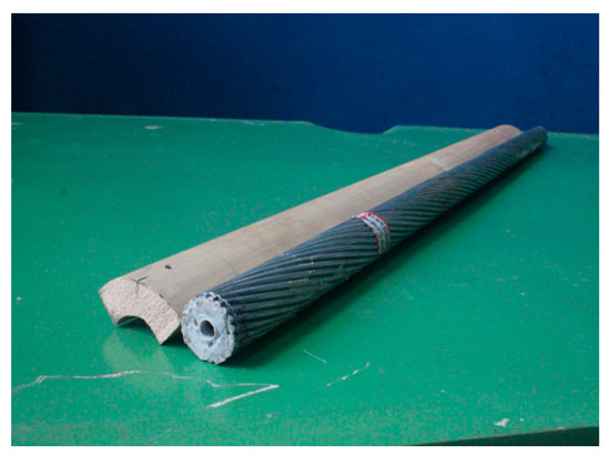
Figure 3.
Test transmission conductor.
2.2. Test Equipment
2.2.1. Wind Tunnel
The tests of the iced conductor were performed in a 1.4 × 1.4 m direct-action wind tunnel, as indicated in Figure 4a. The conductor force test model was mounted vertically on a special support device located in the center of the turntable in the wind tunnel test section (Figure 4b). The wind tunnel was a DC low-speed wind tunnel with a wind speed range of 0–65 m/s. The conductor model was in the center of the wind tunnel. Through observation of the galloping of the transmission line in operation, it was observed that the wind speed range was normally within 4~20 m/s, and the transmission line would gallop. The initial angle of wind attack was 0°, and various angles of wind attack between 0° and 180° were employed during the wind tunnel test to gauge the aerodynamic coefficients. The increment was set at 5° (considering the expense of the wind tunnel test).
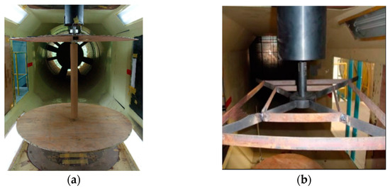
Figure 4.
Aerodynamic force measurement test system for iced conductor: (a) wind tunnel test; (b) test model support device.
2.2.2. Measurement and Control Equipment
In this test, TG0151A and TG0151B balances were used to measure the drag, lift, and moment coefficients of the conductor model. The PXI system was selected for the force test data acquisition system of iced conductors. Angle control and speed pressure control were realized by the corresponding industrial computer system. Instructions were passed between devices by network communication.
The iced conductor galloping characteristics measurement instruments included a dynamic signal analyzer, an acceleration sensor, a linear array CCD, etc. The accelerometer measured the natural frequency of lateral vibration and the natural frequency of torsional vibration of the dancing test model; the data were displayed, stored, and analyzed in real time through the dynamic analysis system; and the linear CCD measured the galloping response signal.
3. Fundamentals of Neural Network
3.1. BP Neural Network
The error backpropagation network (BP neural network) model was put forth by Rumelhart et al. in 1985. Three layers make up the BP neural network: the input layer, the hidden layer, and the output layer. The two steps of its training learning process—signal forward propagation and error backpropagation—can be separated. The BP neural network is one of the most well-liked neural network models. Figure 5 depicts the BP neural network structure framing diagram.
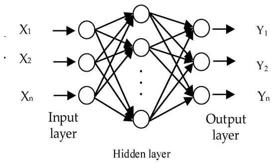
Figure 5.
BP neural network structure framing diagram.
Signal forward transmission: For any hidden layer neuron j, its input is as follows:
where is a weighted result between an input layer neuron i and a hidden layer neuron j, and is the input variable.
Error backpropagation: According to the accumulated error, the modified weighted result is obtained by the gradient descent method:
where η is the learning rate of the set error direction propagation and D is the cumulative error between the actual output of the hidden layer and the desired output.
3.2. Neural Network Parameters
- (1)
- Creation Function and Activation Function
The newff function was used to establish a neural network, in which the number of network layers and the number of neurons in each layer were determined, and the corresponding activation function is given. This article uses logsig and tansig activation functions.
- ➀
- logsig activation function:
- ➁
- tansig activation function:
- (2)
- Learning function and training function
The learning function was used to modify the weights between neurons and the threshold value within neurons and finally achieve local optimization. The L-M optimization algorithm has advantages for function fitting problems, and its prediction accuracy was verified in the simulation example session. Therefore, the L-M optimization algorithm was used as the training function to train the model.
- (3)
- Loss function
The loss function is an operation function that measures the degree of difference between the predicted and actual results of a model. Using the data from the wind tunnel test, the accuracy of the sample data described by the prediction model was determined by the mean squared error loss function (MSE).
where y represents the predicted results, z is the number of test results, and N is the sample.
4. Database Creation
4.1. Determination of the Input Feature Parameters
The lift, drag, and moment coefficients of the iced conductor are represented by the following definitions:
The aerodynamic coefficients indicate the force of the external environmental wind load, where FD is the drag on the iced conductor, FL is the lift, FM is the moment, ρ indicates air density, and U indicates wind speed. The length of the iced conductor model is represented by L, and its diameter by D. In this paper, CL is the same as Cl, CD is the same as Cd, and CM is the same as Cm. Additionally, the direction of the wind affects the aerodynamic coefficients of the conductor (the angle between the mainstream direction of the wind and the horizontal plane). Therefore, these three influencing factors were determined to be the input characteristic parameters of the neural network.
4.2. Model Building
The settings and experimental findings from the wind tunnel test are utilized as example sources in this paper. The input parameters include wind speed, ice thickness, and angle of wind attack. The output parameters are the moment, drag, and lift coefficients. Training of the sample data was started after importing the training set into the Neural Network Fitting toolbox. The most precise training model was determined by observing the training results based on the MSE values. After adding the necessary data to the trained model, the prediction outcome could ultimately be obtained.
- (1)
- The number of model layers and neurons
The model consisted of a three-layer network with an input layer, a hidden layer, and an output layer. From the sample data, both the input and output variables were three-dimensional, and both the input and output layers were set to three neurons. According to the empirical formula and trial and error method, the number of hidden layer nodes of the reasonable BP neural network model was determined, and when the hidden layer was set to 10 neurons, the mean squared error of the prediction result was the smallest. Therefore, it was established that there are 10 hidden layer neural network nodes overall.
- (2)
- Parameter settings
The model was trained using the L-M optimization process, and the error was calculated using the average square error algorithm. By default, the model allows up to 1000 iterations, with a maximum target error of 0.001 and a learning rate of 0.01.
4.3. Model Training
The training data had to be normalized before training. The Mapminmax function was used during the experiment to perform the procedure. The data range was [−1,1]. The processed data were randomly divided into three groups in the proportion of 70%, 15%, and 15% for the training set, verification set, and test set, respectively. After the training model was completed, the error transformation during network training could be observed through the performance interface. The training state interface in the network training process displayed the gradient transformation, Mu factor size, and generalization capacity. The regression ability of data of the network was shown through the regression interface. The numerical size of the MSE was observed through parameter adjustment. Until the target forecast was reached, the mean square error was within 10%.
5. Prediction Results of the Neural Network of the Aerodynamic Coefficients of the Iced Conductor
A portion of the data were chosen as the training data based on the data collected during the test in the wind tunnel, and the rest were used as the test data. The training data were imported into the neural network prediction model for training, and the prediction data were generated.
5.1. Steady Aerodynamic Coefficients Prediction
From the steady data, the aerodynamic coefficients of crescent-shaped iced conductors with ice thicknesses of 12 mm, 20 mm, and 28 mm at 14 m/s wind speed were selected. The aerodynamic coefficients of crescent-shaped iced conductors under 12 mm ice thickness and wind speeds of 10 m/s, 12 m/s, and 18 m/s were also selected.
5.1.1. Ice Thicknesses
The aerodynamic coefficients of crescent-shaped iced conductors with the same wind speed were predicted under different ice thicknesses. The angle of wind attack and the ice thickness were input variables, and the lift, drag, and moment coefficients were output variables.
As seen in Figure 6, the linear regression law of the aerodynamic coefficients of the crescent-shaped iced conductor was essentially the same with ice thicknesses of 12 mm, 20 mm, and 28 mm under the wind speed of 14 m/s. The lift coefficients displayed an increasing trend between 0° and 35° and between 120° and 60° and a downward trend at 35°~120° and 160°~180°. The drag coefficients showed a downward trend at 0°~10° and 85°~165° and an upward trend at 10°~85° and 165°~180°. The moment coefficients showed an upward trend at 0°~40° and 160°~180° and a downward trend at 40°~160°.
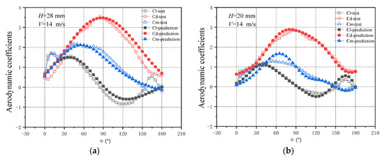
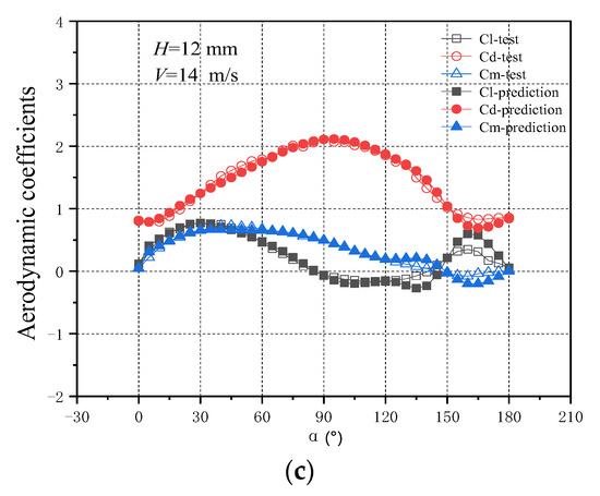
Figure 6.
Steady aerodynamic coefficients under different ice thicknesses.
Under the crescent wind speed of 14 m/s, the aerodynamic parameters under the ice thicknesses of 28 mm, 20 mm, and 12 mm were predicted (Figure 6a–c, respectively).
In Figure 6a, the predicted moment coefficient result at an angle of wind attack of 0°~20° is lower than the wind tunnel result, while the predicted lift coefficient result is slightly higher than the wind tunnel result. The predicted drag coefficient result is also slightly higher than the wind tunnel result. When the wind attack angle is 15°, the loading surface of the iced conductor is the largest, and according to the principle of Bernoulli, the lift coefficients and moment coefficients will increase significantly at this time. The gradient of change in the sample data is too obvious, and there is a large local difference in Figure 6a. In Figure 6b, the predicted results of the lift coefficient and the drag coefficient fit well, and the predicted results of the moment coefficient are slightly lower than the wind tunnel result at 0°~50°, while the predicted results at 50°~90° are higher than the wind tunnel results. Figure 6c shows that the drag coefficients and moment coefficients have good predictive abilities, whereas the lift coefficient predictions for the angles of attack of 125°~150° and 150°~180° are marginally higher and lower, respectively, than the wind tunnel data. There are some inflection points in the prediction data, but the overall linearity is similar; the locally existing prediction differences are within control, and the prediction results meet the expectations.
5.1.2. Wind Speeds
Using crescent-shaped iced conductors of the same ice thickness as the research object, the aerodynamic coefficients for various wind speeds were predicted.
As seen in Figure 7, under speeds of 10 m/s, 12 m/s, and 18 m/s, the linear regression law of the aerodynamic coefficients of the crescent-shaped iced conductor was essentially the same. The lift coefficients of the crescent-shaped iced conductor showed an upward trend at 0°~30° and 125°~160° and a downward trend at 30°~125° and 160°~180°. The drag coefficients showed an upward trend at 0°~100°, 130°~145°, and 150°~160° and a downward trend at 0°~10°, 130°, 145°~150°, and 160°~180°, as well as a downward trend at 0°~10° and 85°~165°. The moment coefficients showed an upward trend at 0°~40° and 160°~180° and a downward trend at 40°~160°.
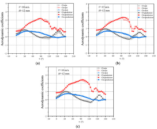
Figure 7.
Steady aerodynamic coefficients at different wind speeds.
With a crescent-shaped iced thickness of 12 mm, aerodynamic coefficients were predicted under wind speeds of 18 m/s, 12 m/s, and 10 m/s (Figure 7a–c, respectively). According to the Reynolds number calculation formula, the Reynolds numbers at wind speeds of 10, 12, and 18 m/s were 488,108, 585,730, and 878,595, respectively.
The predicted results of the aerodynamic coefficients in Figure 7a fit well with the wind tunnel results, especially the drag coefficients at 90°~180° predicting the change in the wind tunnel results. In Figure 7b, the overall fit of the predicted results of the lift coefficients and the moment coefficients is good, and the predicted results of the drag coefficients are slightly higher than the wind tunnel results at 90°~120°, while the predicted results at 120°~150° are lower than the wind tunnel results. Since the crescent-shaped iced conductor is a non-circular segment, the drag coefficients will increase when the conductor is on the windward side and fall when it is on the leeward side. In Figure 7c, the overall linear fit of the aerodynamic coefficients is high, and the prediction results are good and meet the expectations.
5.2. Unsteady Aerodynamic Coefficients Prediction
In the dynamic test, the conductor was placed in the wind tunnel, and the torsional vibration of the conductor force test model was driven by the special drive mechanism. From the unsteady data, at conductor frequencies of 0.1 Hz, 0.2 Hz, and 0.3 Hz, the aerodynamic coefficients of the crescent-shaped iced conductor at a wind speed of 10 m/s and an ice thickness of 14.5 mm were chosen.
At a wind speed of 10 m/s and an ice thickness of 21.5 mm, the aerodynamic coefficients of the sector-shaped iced conductor were chosen at conductor frequencies of 0.1 Hz, 0.2 Hz, and 0.3 Hz. The aerodynamic coefficients of the crescent-shaped iced conductor with wind speeds of 10 m/s, 12 m/s, 14 m/s, and 18 m/s were selected at an ice thickness of 14.5 mm and a frequency of 0.1 Hz. At wind speeds of 10 m/s, 12 m/s, 14 m/s, and 18 m/s, the aerodynamic coefficients of the sector-shaped conductor at an ice thickness of 21.5 mm and a frequency of 0.1 Hz were chosen. With a wind speed of 10 m/s and a frequency of 0.1 Hz, the aerodynamic coefficients of crescent-shaped conductors with ice thicknesses of 14.5 mm, 24 mm, and 33 mm, were chosen, and sector-shaped iced conductors with ice thicknesses of 21.5 mm and 30 mm.
5.2.1. Ice Thicknesses
Based on crescent-shaped and sector-shaped iced conductors with the same wind speed and frequency, the aerodynamic coefficients of the conductors under various ice thicknesses were estimated. The linear regression equation of the aerodynamic coefficients of the various conductor thicknesses was essentially the same, as illustrated in Figure 8, when the wind speed was 10 m/s and the frequency was 0.1 Hz. In general, the lift coefficients and moment coefficients of crescent-shaped iced conductors evolved similarly, with an upward trend at −30°~45° and a decreasing trend at −45°~30°. The drag coefficients at −45°~10° showed a downward trend and showed an upward trend at 10°~45°. The lift coefficients of the sector-shaped iced conductor continued to decrease from −45° to 45°. The drag coefficients showed an upward trend at −45°~0° and a downward trend at 0°~45°. The overall change in moment coefficients was gentle and slowly decreased at 20°~45°.
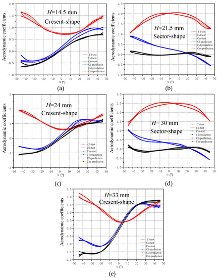
Figure 8.
Unsteady aerodynamic coefficients under different ice thicknesses.
The aerodynamic coefficients from the test results changed in a narrow range and were smooth, as shown in Figure 8a–e, with a good prediction result. The prediction data fit well and met the expectations of the prediction results.
5.2.2. Wind Speeds
Using iced conductors in crescent and sector shapes that had the same ice thickness and frequency as the research items, the aerodynamic coefficients at various wind speeds were estimated. The linear regression law of the aerodynamic coefficients in the conductors of various ice thicknesses was essentially the same, as illustrated in Figure 9. The lift coefficients indicated a negative trend at −45°~30° and 35°~45° and an increasing trend at −30°~35°. The moment coefficients generally increased. The drag coefficients showed a downward trend at −45°~10° and an upward trend at 10°~45°. The lift coefficients of the sector-shaped iced conductors continued to decrease overall. The drag coefficients showed an upward trend at −45°~−10° and a downward trend at −10°~45°. The moment coefficients fluctuated around zero overall. According to the Reynolds number calculation formula, the Reynolds numbers at wind speeds of 10, 12, 14, and 18 m/s were 488,108, 585,730, 683,351, and 878,595, respectively.
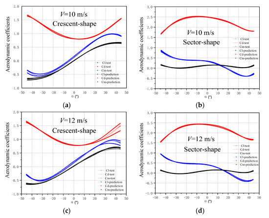
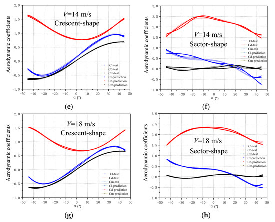
Figure 9.
Unsteady aerodynamic coefficients at different wind speeds.
5.2.3. Frequencies
The aerodynamic coefficients of the conductors under different frequencies were predicted using iced conductors with the same ice thickness and wind speed as the research objects. As shown in Figure 10, the linear regression law of the aerodynamic coefficients at various frequencies was essentially the same. The lift coefficients and moment coefficients of the conductors generally increased. The drag coefficients showed a downward trend at −45°~0° and an upward trend at 0°~45°. The lift coefficients and moment coefficients of the conductors showed an overall downward trend. The drag coefficients showed an upward trend at −45°~−10° and a downward trend at −10°~45°.
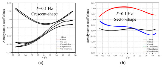
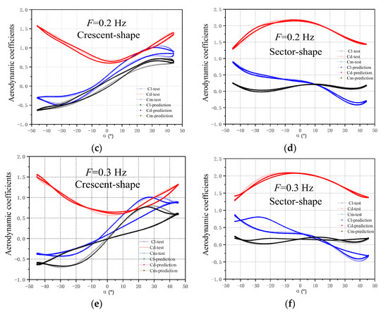
Figure 10.
Aerodynamic coefficients at different frequencies.
Figure 10a,b,d,f show a good prediction effect and a high degree of fit. In Figure 10c,e, at the angle of wind attack of 25°~45°, the prediction results are quite different from the test data. Since the dynamic wind tunnel test will have different results at the same wind attack angle, it has a greater impact on the training of the prediction model.
The results show that the change law of the prediction result and the data change curve obtained by the wind tunnel test have good consistency. In addition, factors such as the span of input coefficients of the neural network, the amount of sample data, and the amount of data value variation have a direct impact on the prediction effect. The average square error of the prediction result was within 10%, which realizes the prediction expectation.
5.3. Prediction Error Analysis
Mean square error (MSE) is a measure of the discrepancy of an estimator, and the estimator is calculated in machine learning. An ideal model has a value of 0 when the projected value and the actual value agree completely. The larger the inaccuracy is, the higher the value is. The more accurate the machine learning network model is, the lower the value will be. The mean squared error of the steady and unsteady aerodynamic coefficients from the prediction experiment was calculated using Equation (5).
The prediction results of the crescent steady aerodynamic coefficients are shown in Table 1, the prediction results of the crescent unsteady aerodynamic coefficients are shown in Table 2, and the prediction results of the sector unsteady aerodynamic coefficients are shown in Table 3.

Table 1.
Prediction results of the crescent steady aerodynamic coefficients.
Table 2.
Prediction results of the crescent unsteady aerodynamic coefficients.
Table 3.
Prediction results of the sector unsteady aerodynamic coefficients.
5.4. Den Hartog Coefficients and Nigol Coefficients
When the aerodynamic coefficients of the iced conductors meet Equations (9) and (10), the Den Hartog vertical galloping and Nigol torsion galloping criteria are applied. Vertical galloping or torsional self-excited galloping of the iced conductors may be caused.
where CL represents the coefficients of lift, CD indicates drag coefficients, and α indicates the angle of wind attack.
where CM represents the moment coefficients and α indicates the angle of wind attack.
The aerodynamic coefficients of the crescent-shaped iced conductor derived by the neural network prediction approach and test are displayed in Figure 11 and were used to calculate the Den Hartog and Nigol coefficients.
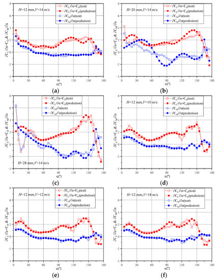
Figure 11.
Den Hartog coefficients and Nigol coefficients of crescent-shaped iced conductor.
Figure 11a shows the Den Hartog vertical galloping mechanism and the Nigol torsion galloping mechanism in the 160°~180° wind attack angle range. The iced conductor may face vertical galloping in the 65°~160° angle of wind attack range. In Figure 11b, in the 120°~180° range of angle of wind attack, the iced conductor may face vertical galloping, and the 60°~165° range of angle of wind attack may cause the iced conductor to face torsion galloping. In Figure 11c, in the range of angle of wind attack of 160°~180°, the iced conductor may face vertical galloping, and the range of 45°~135° and near 150° may cause the iced conductor to face torsion galloping. In Figure 11d, in the 160°~180° range of angle of wind attack, the iced conductor may face vertical galloping, and near the angle of wind attack of 140°, the iced conductor may face torsion galloping. In Figure 11e, in the range of angle of wind attack of 160°~180°, the iced conductor may face vertical galloping, and the 45°~135° angle of wind attack range may cause the iced conductor to face torsion galloping. In Figure 11f, in the range of angle of wind attack of 160°~180°, the conductor may face vertical galloping, and the range of 85°~135° may cause the iced conductor to face torsion galloping. The thickness of the ice has a greater influence on the Nigol coefficients, and the wind speed has a smaller influence on the Den Hartog and Nigol coefficients. Both the neural network predictions and the wind tunnel test results show that when the crescent-shaped iced conductor is in torsional motion, it may also undergo galloping without satisfying the Den Hartog mechanism.
Based on the machine learning method, in order to further demonstrate the viability of the neural network prediction approach, the aerodynamic coefficients of the iced conductors were anticipated. The findings of the test were then compared with the analysis of the Den Hartog and Nigol coefficients. The following conclusions have been obtained: using the neural network and wind tunnel test, crescent-shaped iced conductors were used to derive the Den Hartog and Nigol coefficients. Galloping was brought on by the Den Hartog and Nigol coefficients, which are also important in preventing it. Therefore, research on the galloping of the conductors and technologies for prevention and control can make use of neural network methods to anticipate the aerodynamic coefficients of iced conductors.
6. Conclusions
The steady and unsteady aerodynamic coefficients of iced conductors were acquired from a wind tunnel test. Machine learning was used to build a prediction model. The results of the wind tunnel test were contrasted with those predicted. The galloping characteristics obtained by the two methods were further analyzed.
- (1)
- The input parameter range, the volume of sample data, and the degree of data numerical volatility all directly affect the prediction effect. The mean square error of the prediction results obtained based on the neural network prediction method is within 10%, which realizes the prediction expectation.
- (2)
- The greater the thickness of the ice is at the same wind speed, the greater is the fluctuation of the aerodynamic coefficients in the range of the angle of wind attack. Different wind frequencies and speeds under the same ice thickness conditions have little impact on the change in lift and drag coefficients of an iced conductor. It is also important to note that they have little effect on the torque coefficients.
- (3)
- Based on machine learning and the wind tunnel test, the aerodynamic coefficients were calculated and analyzed. Additionally, the coefficients of Den Hartog and Nigol were calculated and analyzed to change with the angle of wind attack, which verified the feasibility of machine learning to predict the gallop characteristics.
In this paper, using the wind tunnel test, the steady and unsteady aerodynamic coefficients under various conditions were derived. A prediction method of aerodynamic coefficients under the wind load of iced wind of transmission lines is proposed. This study successfully addresses the issue of expensive and prolonged wind tunnel tests. Additionally, it helps avoid and manage iced transmission line galloping.
Author Contributions
Conceptualization, M.C. and J.L. (Junhao Liang); methodology, Q.W.; software, L.Z.; validation, H.H.; formal analysis, M.C.; investigation, J.L. (Jun Liu); resources, G.M.; data curation, Q.W.; writing—original draft preparation, J.L. (Junhao Liang); writing—review and editing, J.L. (Junhao Liang); visualization, H.H.; supervision, M.C.; project administration, M.C.; funding acquisition, M.C. All authors have read and agreed to the published version of the manuscript.
Funding
This work was financially supported by the National Natural Science Foundation of China (51507106); the Postdoctoral Research Foundation of China (51507106); Chengdu International Science and Technology Cooperation Support Funding (2020-GH02-00059-HZ); and the Open Research Fund of Failure Mechanics and Engineering Disaster Prevention, Key Laboratory of Sichuan Province, Sichuan University (FMEDP202201).
Data Availability Statement
The data presented in this study are available in this article.
Conflicts of Interest
The authors declare no conflict of interest.
References
- Cai, M.Q.; Yan, B.; Lu, X.; Zhou, L.S. Numerical simulation of aerodynamic coefficients of iced-quad bundle conductors. IEEE Trans. Power Deliv. 2015, 30, 1669–16126. [Google Scholar] [CrossRef]
- Cai, M.Q.; Xu, Q.; Zhou, L.S.; Liu, X.H.; Huang, H.J. Aerodynamic characteristics of iced 8-bundle conductors under different turbulence intensities. KSCE J. Civ. Eng. 2019, 23, 4812–4823. [Google Scholar] [CrossRef]
- Cai, M.Q.; Zhou, L.S.; Lei, H.; Huang, H.J. Wind tunnel test investigation on unsteady aerodynamic coefficients of iced 4-bundle conductors. Adv. Civ. Eng. 2019, 2019, 2586242. [Google Scholar] [CrossRef]
- Zhang, M.J.; Xu, F.Y. Tuned mass damper for self-excited vibration control: Optimization involving nonlinear aeroelastic effect. J. Wind Eng. Ind. Aerodyn. 2022, 220, 104836. [Google Scholar] [CrossRef]
- Zhang, M.J.; Wu, T.; Oiseth, O. Vortex-induced vibration control of a flexible circular cylinder using a nonlinear energy sink. J. Wind Eng. Ind. Aerodyn. 2022, 229, 105163. [Google Scholar] [CrossRef]
- Meng, Y.B.; Zou, J.H.; Gan, X.S.; Zhao, L. Research on WNN aerodynamic modeling from flight data based on improved PSO algorithm. Neurocomputing 2012, 83, 212–221. [Google Scholar] [CrossRef]
- Wang, Q.; Wu, K.Y.; Zhang, T.J.; Kong, Y.N.; Qian, W.Q. Aerodynamic modeling and parameter estimation from QAR data of an airplane approaching a high-altitude airport. Chin. J. Aeronaut. 2012, 25, 361–3121. [Google Scholar] [CrossRef]
- Raeesi, A.; Cheng, S.H.; Ting, D.S.K. Aerodynamic damping of an inclined circular cylinder in unsteady flow and its application to the prediction of dry inclined cable galloping. J. Wind Eng. Ind. Aerodyn. 2013, 113, 12–28. [Google Scholar] [CrossRef]
- Ignatyev, D.I.; Khrabrov, A.N. Neural network modeling of unsteady aerodynamic characteristics at high angles of attack. Aerosp. Sci. Technol. 2015, 41, 106–115. [Google Scholar] [CrossRef]
- Wang, J.; Xiong, X.F.; Zhou, N.; Li, Z.; Wang, W. Early warning method for transmission line galloping based on SVM and AdaBoost bi-level classifiers. IET Gener. Transm. Distrib. 2016, 10, 3499–35012. [Google Scholar] [CrossRef]
- Lee, J.; Jung, H.Y.; Koo, J.R.; Yoon, Y.; Jung, H.J. Prediction of galloping accidents in power transmission line using logistic regression analysis. J. Electr. Eng. Technol. 2017, 12, 969–980. [Google Scholar] [CrossRef][Green Version]
- Ma, W.Y.; Macdonald, J.H.G.; Liu, Q.K.; Nguyen, C.H.; Liu, X.B. Galloping of of an elliptical cylinder at the critical Reynolds number and its quasi-steady prediction. J. Wind Eng. Ind. Aerodyn. 2012, 168, 110–122. [Google Scholar] [CrossRef]
- Winter, M.; Breitsamter, C. Nonlinear identification via connected neural networks for unsteady aerodynamic analysis. Aerosp. Sci. Technol. 2018, 1212, 802–818. [Google Scholar] [CrossRef]
- Li, K.; Kou, J.Q.; Zhang, W.W. Deep neural network for unsteady aerodynamic and aeroelastic modeling across multiple Mach numbers. Nonlinear Dyn. 2019, 96, 21512–211212. [Google Scholar] [CrossRef]
- Wang, X.; Kou, J.Q.; Zhang, W.W. Unsteady aerodynamic modeling based on fuzzy scalar radial basis function neural networks. Proc. Inst. Mech. Eng. Part G–J. Aerosp. Eng. 2019, 233, 51012–55121. [Google Scholar] [CrossRef]
- Chen, H.; He, L.; Qian, W.Q.; Wang, S. Multiple aerodynamic coefficient prediction of airfoils using a convolutional neural network. Symmetry 2020, 12, 544. [Google Scholar] [CrossRef]
- Jaffar, F.; Farid, T.; Sajid, M.; Ayaz, Y.; Khan, M.J. Prediction of drag force on vehicles in a platoon configuration using machine learning. IEEE Access 2020, 8, 201823–201834. [Google Scholar] [CrossRef]
- Mannini, C. Incorporation of turbulence in a nonlinear wake-oscillator model for the prediction of unsteady galloping response. J. Wind Eng. Ind. Aerodyn. 2020, 200, 104141. [Google Scholar] [CrossRef]
- Mou, Z.Y.; Yan, B.; Yang, H.X.; Cai, D.D.; Huang, G.Z. Prediction model for aerodynamic coefficients of iced quad bundle conductors based on machine learning method. R. Soc. Open Sci. 2021, 8, 210568. [Google Scholar] [CrossRef]
- Rykaczewski, D.; Nowakowski, M.; Sibilski, K.; Wroblewski, W.; Garbowski, M. Identification of longitudinal aerodynamic characteristics of a strake-wing micro aerial vehicle by artificial neural networks. Bull. Pol. Acad. Sci.-Tech. Sci. 2021, 69, 9. [Google Scholar] [CrossRef]
- Yu, H.Y.; Xu, F.Y.; Zhang, M.J.; Zhou, A.Q. Experimental investigation on glaze ice accretion and its influence on Aerody Namic characteristics of pipeline suspension bridges. Appl. Sci. 2020, 10, 7167. [Google Scholar] [CrossRef]
- Xu, F.Y.; Yu, H.Y.; Zhang, M.J.; Han, Y. Experimental study on aerodynamic characteristics of a large-diameter ice-accreted cylinder without icicles. J. Wind Eng. Ind. Aerodyn. 2021, 208, 104453. [Google Scholar] [CrossRef]


Disclaimer/Publisher’s Note: The statements, opinions and data contained in all publications are solely those of the individual author(s) and contributor(s) and not of MDPI and/or the editor(s). MDPI and/or the editor(s) disclaim responsibility for any injury to people or property resulting from any ideas, methods, instructions or products referred to in the content. |
© 2022 by the authors. Licensee MDPI, Basel, Switzerland. This article is an open access article distributed under the terms and conditions of the Creative Commons Attribution (CC BY) license (https://creativecommons.org/licenses/by/4.0/).