Abstract
As-built progress of the constructed pavement should be monitored effectively to provide prompt project control. However, current pavement construction progress monitoring practices (e.g., data collection, processing, and analysis) are typically manual, time-consuming, tedious, and error-prone. To address this, this study proposes sensors mounted using a UGV-based methodology to develop a pavement layer change classifier measuring pavement construction progress automatically. Initially, data were collected using the UGV equipped with a laser ToF (time-of-flight) distance sensor, accelerometer, gyroscope, and GPS sensor in a controlled environment by constructing various scenarios of pavement layer change. Subsequently, four Long Short-Term Memory network variants (LSTMs) (LSTM, BiLSTM, CNN-LSTM, and ConvLSTM) were implemented on collected sensor data combinations for developing pavement layer change classifiers. The authors conducted the experiment to select the best sensor combinations for feature detection of the layer change classifier model. Subsequently, individual performance measures of each class with learning curves and confusion matrices were generated using sensor combination data to find out the best algorithm among all implemented algorithms. The experimental result demonstrates the (az + gx + D) sensor combination as the best feature detector with high-performance measures (accuracy, precision, recall, and F1 score). The result also confirms the ConvLSTM as the best algorithm with the highest overall accuracy of 97.88% with (az + gx + D) sensor combination data. The high-performance measures with the proposed approach confirm the feasibility of detecting pavement layer changes in real pavement construction projects. This proposed approach can potentially improve the efficiency of road construction progress measurement. This research study is a stepping stone for automated road construction progress monitoring.
1. Introduction
Most pavement construction projects often suffer from time and cost overruns due to associated risks in the construction stage [1,2]. Efficient construction progress monitoring (CPM) is vital to enable the as-built progress status of the project by comparing as-built progress with as-planned progress throughout the project for project control [3,4]. The as-built progress measurement is measured for the construction of different road layers (e.g., subgrade, subbase, base, and surface) and then combined along the road project length to evaluate overall pavement construction progress. [5,6]. During this process, each constructed (as-built) road layer with corresponding spatial information (starting and finishing points) is identified and utilized for as-built measurement.
Traditionally, this process is manually carried out, which is characterized by text-based data collection and manual checklists. Project managers typically spend 30–50% of their time gathering and analyzing these as-built collected data [7]. As such, manual CPM is criticized for being manual, tedious, error-prone, and time-consuming [8]. Subsequently, recent technological developments introduced several automated data collection technologies to capture as-built data of pavement construction with less manual intervention. Examples include technologies such as the Global Navigation Satellite System (GNSS), total station, sensor (LiDAR and RGB camera)-equipped unmanned aerial vehicle (UAV) [2,3,9,10,11]. However, the collected as-built data are manually analyzed in the form of point clouds, aerial images, and surveyed data (for example, total station and GNSS) [3,9,12,13]. The interpretation of these data may be inconsistent, subjective, and time-consuming [12,14]. Despite the efficiency gains, as-built component detection remains complex, manual, or semiautomated, which causes delays in the project controlling action [2,12].
Road pavement construction is characterized by its repetitive nature, consisting of activities that are sequentially repeated along the road length, such as constructing various road pavement layers along the road length, including the surface layer, base course layer, subbase layer, and subgrade layer [4,12]. Hence, automated road layer detection is quite crucial information for automated road construction progress monitoring [12]. Despite the importance of automated layer detection, only two research studies have attempted to detect as-built road layers automatically for automated road construction progress measurement. Vick and Brilakis (2018) and Lo et al. (2022) investigated automated road layer detection from point cloud data using a UAV photogrammetry-based 3D reconstruction approach. Both studies strongly support the road layer detection approach to measuring road progress monitoring. However, the proposed 3D construction-based approach is, unable to detect the thin road layer (i.e., asphalt), susceptible to vertical occlusions, and not applicable to segment-wise construction [13,15]. It is also noted that the feasibility of UAV is deterred due to the requirement of training, skill, safety concerns, and complex regulatory approval processes, especially in no-fly zones (control zones, areas of military operations, and restricted areas) [10,16]. Drone operation is forbidden in more than 20 nations, such as Bhutan, Algeria, Kuwait, Bahrain, Egypt, and Cuba [17,18,19,20]. The UGV has evolved as a solution to resolve the issues faced by UAVs and can be operated in a diverse construction environment with fewer safety concerns. Similarly, sensors (motion and distance) can be a better alternative than a vision-based 3D reconstruction approach to detect the features from motion patterns using deep learning techniques for road layer change detection [10].
The as-built progress measurement of road construction requires the information of as-built pavement layer(s) with corresponding spatial information with respect to time, considering the repetitive nature of the road. Hence, road layer detection is quite crucial information for as-built road construction progress measurement. During the construction, various road layers can be detected from their interrelationship with the layer change information along the road length. The scope of the proposed study is only to develop a pavement layer change classifier. Therefore, this paper proposes a novel solution to implement sensors mounted unmanned ground vehicle (UGV) to automate layer change detection by developing a layer change classifier using deep learning techniques for as-built road layer detection. In order to achieve this, the following research objectives were accomplished:
- (1)
- To develop the layer change classifier to detect the pavement layer change automatically using sensors mounted UGV prototype and four main Long Short-Term Memory techniques (LSTMs).
- (2)
- To determine the best combinations of sensors to consider as optimum feature detectors for developing the pavement layer change classifiers.
- (3)
- To examine the LSTM feasibility to detect the road layer change and find the best-performing LSTM network for developing a layer change classifier.
This study proposes an automated approach to detect road layer changes using sensors (accelerometer, gyroscope, ToF sensor, and GPS sensors) mounted UGV and deep learning techniques for road layer detection. Initially, the dataset was generated in a controlled environment by simulating (by physically creating the road) the road layer changes with different combinations of road layers, corresponding thicknesses, and adjoining slopes. Subsequently, four pavement layer change classifiers were developed to detect the road layer change from collected sensor data using LSTM, BiLSTM, CNN LSTM, and ConvLSTM networks. The effectiveness of sensor combinations was assessed by comparing their performance with classifiers. The optimum LSTM was also evaluated by comparing the performance of classifier models to detect road layer change.
2. Literature Review
2.1. Automated as-Built Data Collection Technologies
Researchers have widely utilized sensors such as motion sensors, distance sensors, time-lapse cameras, depth cameras, and LiDAR, mounted on mobile (i.e., UAV and equipment) and fixed platforms to collect as-built data for constructed component detection [9,10,21,22]. Rao et al. (2022) and Omar and Nehdi (2016) stated that mobile platforms are proven more favorable for mounting sensors, especially in horizontal infrastructure, because of unique benefits such as speedy data acquisition, more coverage of construction sites, and no need for the installation of many sensors along the length [10,23]. Despite having many benefits and great popularity, aerial data collected with UAVs are challenged in the construction industry by restrictions due to safety issues, licensing, and training requirements sanctioned by the government, local bodies and aviation authorities [10,16,24]. Many countries consist of complex and time-consuming approval processes for drone operations, such as New Zealand and India [25,26]. By resolving these issues, UGV has started to receive the attention of researchers due to greater flexibility [16]. Recent studies, such as Kim et al. (2019), Asadi et al. (2020), and Park et al. (2019), strongly confirmed the viability of the UGV as a platform to equip sensors for automated data collection in construction [16,27,28]. On the other hand, Ryu et al. (2019) and Kim and Cho (2020) reported that motion sensor data typically require less computational power to process and analyze compared to imaging sensors generating the image, point cloud, and video data [29,30]. Additionally, occlusion problems (i.e., line of sight) can be avoided with motion sensor data, which is a bigger issue with vision-based approaches [30]. Consequently, the motion-sensing approach is an increasingly embraced choice that bolsters the impetus to equip motion sensors for pattern detection based on progress monitoring in construction [31].
2.2. As-Built Object Detection in the CPM Domain
Conventional methods adopt manual visual inspection to assess the as-built construction for CPM, which may be time-consuming, laborious, dangerous, and inaccurate [32]. Automated object recognition has been widely researched to recognize the status of projects, activity recognition, as-built quantity estimation, and productivity analysis in the CPM domain [11,33,34,35]. Many CPM-related studies have investigated building information modelling (BIM) and point cloud-based automated as-built component detection of vertical buildings, e.g., Golparvar-Fard et al. (2011), Turkan et al. (2012), Bosche et al. (2015), and Braun and Borrmann (2019) [36,37,38]. Techniques such as the global descriptor, semi-global-matching (SGM) algorithm, and iterative closest point (ICP) algorithm have been used to detect the as-built components from the point cloud data. However, object detection from the point cloud suffers challenges due to unstructured 3D point cloud data, inconsistent point density, noisy data, cluttered scenes, and computing intensiveness. Patel et al. (2021) identified that most CPM-related studies focused on vertical structures, whereas limited studies investigated road construction progress monitoring [3]. The previous road CPM studies concentrated on earthwork progress [39], productivity [40], and resource activity monitoring [41]. However, these research studies did not concentrate on pavement construction progress measurement, and they also were not able to provide direct physical progress. Subsequently, Vick and Brilakis (2018) researched road layer detection using the UAV-enabled 3D reconstruction process and space-partitioning method [12]. The proposed approach recognizes the road layer by comparing road layer surface elevation from 3D point cloud (as-built data) and BIM 4D (as-planned data). Despite worthy contributions, the study was criticized due to the lack of ability to recognize the thin road layers and having complete reliance on BIM to detect as-built pavement layers. Lo et al. (2022), Costin et al. (2018), and Patel et al. (2021) reported that BIM adoption in road construction is not as widely common as vertical infrastructure [3,13,42]. Consequently, Lo et al. (2022) detected the base course layer of road structure using a UAV-enabled 3D reconstruction technique. Specifically, the proposed method compared the 3D point cloud (as-built) data and AutoCAD files (road geometric design with schedule data) to assess the elevation change at the location for inferring with the road layer [13]. However, it only investigated the soil material for base course layer detection, and the proposed framework was limited to detecting the asphalt layer. Moreover, this approach was also criticized because it cannot be implemented in segment-wise road construction [13,15].
2.3. Machine Learning Techniques in Pattern Detection
Traditional machine learning techniques were researched to detect and classify the patterns of feature data such as random forest (RF), support vector machine (SVM), k-nearest neighbors (k-NN), decision tree (DT), artificial neural network (ANN), and convolutional neural network (CNN) [43]. For example, various labor and equipment activities were recognized in research studies such as [22,29,44,45,46]. The literature review confirms that advanced machine learning techniques, such as deep learning techniques, are capable enough to classify motion sensor-based activity classification with high performance [47,48,49,50]. In particular, research studies such as Slaton et al. (2020), Hernandez and Akhavian (2020), Rashid and Louis (2019), and Deng et al. (2023) [31,51,52,53] have analyzed and confirmed that LSTM and its variant perform well on sequential data with their high capabilities compared to traditional machine learning [47,54]. Moreover, Zhao and Obonyo (2020) utilized convolutional LSTM models [55], and Kim and Cho (2020) used an LSTM network classifier for activity recognition of construction resources [30]. It is evident from previous studies that sensor data were assessed to recognize the activity only, but it is not explored for the as-built completed physical component for CPM.
3. Research Methodology for Layer Change Classifier
As shown in Figure 1, the main three scenarios of pavement layer change commonly observed in road pavement construction are layer not changed, layer up, and layer down. Hence, road layer detection can be carried out with the layer change information and geometric design of road construction.
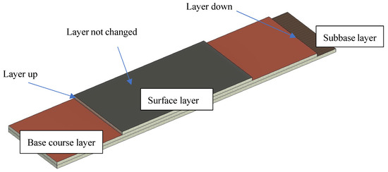
Figure 1.
Layer changes between adjoining road layers along the as-built road length during construction.
In this research study, a layer change classifier model was developed for detecting the road layer changes along the as-built road using sensors mounted on a UGV and deep learning algorithms. Figure 2 shows the overall framework of the research methodology to detect the road layer change classification. To develop a pavement layer change classifier, the research methodology was proposed and described with four main sections: (1) data acquisition, (2) data preprocessing and preparations, (3) constructing supervised machine learning algorithms, and (4) classifier model performance measures for optimum layer change detection classifier.
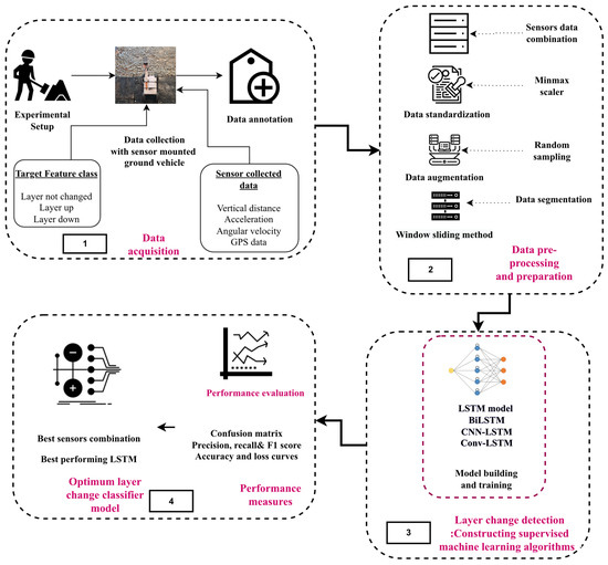
Figure 2.
Overall framework of research methodology of sensors mounted on a UGV to detect road layer change using a deep learning technique.
3.1. Dataset Acquisition
Currently, there is no dataset available to train the machine learning model for developing a road layer change classifier from sensor data. To develop the road layer change classifier, a dataset was generated to train and develop the road layer classifier. The dataset generation was carried out in three steps: (1) configuration of the data collection apparatus, (2) experiment setup, and (3) data collection.
3.1.1. Configuration of Data Collection Apparatus (Sensor Prototype Mounted on UGV)
Motion sensors, e.g., the accelerometer and gyroscope, are also widely equipped to collect data on the kinematic (motion) pattern for activity detection, resource tracking, and construction status [10,21]. Hence, to automate the data collection (layer change) of as-built pavement, sensors were configured on a UGV. During the data collection, sensors mounted UGV collected the motion sensor data and the vertical distance of ToF sensors to the ground to detect the road layer change. Figure 3 illustrates the prototype of the sensors mounted on the unmanned ground vehicle for data acquisition to develop a layer change classifier. In the sensor prototype, four sensors were embedded in the ESP32 circuit: the ToF sensor (VL53L3CX), GPS sensor (NEO-6M), accelerometer, and gyroscope (the accelerometer and gyroscope were combined into MPU6050.). A Wi-Fi module was enabled to transmit and download the data in real time. It should be noted that all sensors data were synchronized.
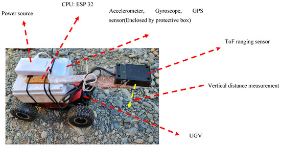
Figure 3.
Sensors mounted on UGV for data collection.
- Embedded sensors
- ToF sensor: Measures the vertical distance from the ToF sensor to the surface of the pavement layer
- Accelerometer: Measures the rate of velocity change of UGV around three axes (x,y,z)
- Gyroscope: Measures angular velocity of UGV around three axes (x,y,z)
- GPS sensor: Measures the geolocation of UGV with longitude and latitude
3.1.2. Experimental Setup
During road pavement construction, three main events were observed for layer change from typical road construction: layer up, layer down, and layer not changed. Road layers can be detected using logical inter-relationships between road pavement layers based on these three events. A large comprehensive dataset is required to train using a deep learning algorithm collected in various pavement construction scenarios consisting of variables to predict the road layer change. With respect to data generation for three main events, typical road construction consists of three main variables (v): road layers (l), corresponding thicknesses (t), and slopes (m), where v ∈ {road layers, thickness, slopes), l∈ {layer1, layer2, layer3, …, layere), t ∈ {thickness1,thickness2,thickness3, …, thicknessg}, m ∈ {slope1,slope2,slope3, …, slopef}. Road layers and their corresponding thicknesses are designed as per the local pavement structure design standards. However, the slope at the edge adjoining two layers is arbitrary and depends on construction practice. Therefore, various slopes and thicknesses were considered to generate the road construction scenarios for dataset generation.
Figure 4 represents the environment of dataset generation, consisting of different road construction scenarios where different road layers with thicknesses were constructed with adjoining slopes to generate the dataset of three events (layer up, layer not changed, and layer down). Three different types of road layer change events were mainly targeted by data generation.
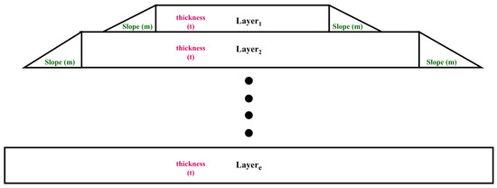
Figure 4.
Dataset generation model to create road layer change data with respect to the main three variables (road layer, thickness, and slope between two adjoining road layers).
3.1.3. Data Collection
Consequently, sensors equipped UGV were run over the various road construction scenarios constructed by different combinations of slopes and road layers (with different thicknesses), registering various sensor data of road layer change events (ToF sensor, accelerometer, gyroscope, and GPS) during its operation. After collecting the data for each scenario, the collected data were transferred through a wireless connection to the workstation. Here, sensor data were converted into CSV format using the standard uniform protocol. Subsequently, data labeling was carried out as layer not changed (same layer), layer down, and layer up according to registered changes with a stopwatch after each scenario.
3.2. Data Preprocessing and Preparations
After the data collection, data preparation was carried out. The collected sensor data were stored in an ESP32 chip embedded in the sensor prototype, and they were transmitted to the laptop for data processing. Subsequently, data labeling was carried out to implement the supervised machine learning algorithm to recognize the pattern of feature classes. Data preparation was carried out in three steps, as described below.
3.2.1. Sensors Data Combination: Input Vector
The collected dataset featured various sensor data (ToF sensors, accelerometer, and gyroscope) consisting of the sequential data pattern for layer change events. Each sensor combination developed a unique dataset that impacted the investigation of layer change detection differently. The investigation process included the implementation of four deep learning algorithms (LSTMs) with sensor combinations to examine the performance of layer change detection for assessing the effectiveness of various sensor combinations.
As illustrated in Figure 5, the combination of each sensor created a feature set that was comprised of seven values: acceleration (three values), angular velocity (three values), and distance (one value). Features sets from various sensor combinations were concatenated to create the input vector. The input vectors were defined individually on the basis of sensors utilized in each sensor combination. There were three input vector formations based on sensor combinations: (1) accelerometer (ax, ay, az) + gyroscope (gx, gy, gz); (2) accelerometer (ax, ay, az) + gyroscope (gx, gy, gz) + distance; (3) 1 axis of the accelerometer (az) + 1 axis of the gyroscope (gx) + distance. It should be noted that all sensor data were concatenated by aligning independent data with timestamps. To evaluate the machine learning classifiers, training and testing data were taken randomly from the generated input vectors, as shown in Figure 5. The sensor combinations were represented in the following manner.
accelerometer (ax, ay, az) + gyroscope (gx, gy, gz) = axyz + gxyz.
accelerometer (ax, ay, az) + gyroscope (gx, gy, gz) + distance= axyz + gxyz + D.
1 axis of accelerometer (az) + 1 axis of gyroscope (gx) + distance= az + gx+ D.
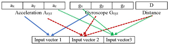
Figure 5.
Feature sets for input vectors.
3.2.2. Data Normalization
In collected sensor data, the distance data had a different scale than the data of acceleration and angular velocity due to a different data range of ToF sensors. Different ranges of the dataset may create the model weight error [38]. Therefore, min–max scaling as a data normalization technique was applied to rescale the data to obtain the same range of data between −1 to 1. Min–max scaling subtracts the minimum value from the highest value of each sensor’s data and then divides it by the data range.
3.2.3. Data Augmentation
The generated dataset may be imbalanced and can create a bias toward a more dominating class with numbers. Therefore, the random oversampling technique was implemented to generate large synthetic data for less populated data classes to balance and augment the dataset [56,57,58]. This process may improve the model generalization by adding data variability without altering the class labels [39]. It may potentially enhance the generalization of the proposed model by introducing data variability without changing the labels [58].
3.2.4. Data Segmentation with Window Sliding Techniques
The data segmentation technique restructures data to form a supervised learning problem for the sequence of time-series dataset numbers. This study implements a sliding window technique to convert segment data from discrete data. Basically, for the considered time-series data si = (si,1, si,2, …, si,l), this techniques segments si into smaller time segments < si,x−d, si,t−x+1, …, si,x, …, si,x+d−1, si,x+d > in x size of the window as the window slides by s (here, d = (x − 1)/2) [31]. The window size may greatly impact the final sequential classification result. Therefore, various window sizes were experimented with to select the size.
3.3. Constructing Supervised Machine Learning Algorithms
Machine learning techniques are broadly researched to classify the pattern of events on the basis of sequential data collected by high-performing kinemetric sensors [47,48]. Sensor-collected data here consisted of the sequential pattern based on features that could classify the main three events (layer not changed, layer up, and layer down) with machine learning algorithms. To categorize various layer change events, supervised deep learning classifiers were utilized here to understand specific patterns. Traditional machine learning algorithms interpret single data into classes, such as SVM classifier, random forest, artificial neural network, k-nearest neighbor, and decision tree. However, the combination of sequential data forms a class with a unique data pattern. Hence, a previous study also confirmed the superiority of recurrent neural networks (such as the LSTM model) compared to the traditional machine learning model [30,59,60,61,62]. Specifically, LSTM and its variant are broadly popular due to their high performance in data mining of sequential sensor data [31,47,63,64]. The performance of these classifiers may vary according to the data and feature types [31,65,66]. Consequently, LSTM, BiLSTM, CNN-LSTM, and ConvLSTM models were implemented and compared to classify the road layer change for this study, as discussed below.
3.3.1. Long Short-Term Memory Network
The LSTM is a widely known technique for analyzing sequential data (time-series data) in predicting trends and classifying features with great performance [67]. In the architecture of the LSTM model classifier, the two-staked LSTM was constructed consisting of two connected LSTM memory cells to deepen the network. The sensor-collected data were sent to a fully connected layer (FCN), which was succeeded by the rectified linear unit (ReLU) layer. Subsequently, two layers of LSTM cells were provided. Output from this process was transmitted to a fully connected layer because the classifier model detects the layer changes at the end of the layer change sequences. Lastly, the generated output from the fully connected layer was forwarded to the Softmax layer to transform the prediction value of the feature class into probability for generating the final detection of the layer change class with the highest probability.
3.3.2. BiLSTM
The Bidirectional Long Term-Short-Term memory (BiLSTM), a sequence processing technique, comprises two LSTMs [66]. Unlike LSTM, a network of BiLSTM consists of two parallel layers in forward and backward propagation directions [68]. The forward LSTM layer obtains preceding features, whereas the backward LSTM layer extracts succeeding features. BiLSTM captures past and forthcoming information to enhance the available context of the proposed algorithm using two individual hidden layers, the forward layer and the backward layer [69]. Subsequently, both hidden states were merged into the final output. The BiLSTM network consisted of the same architecture as the LSTM network; however, the BiLSTM layers (two) existed instead of both LSTM layers in the model network architecture.
3.3.3. CNN-LSTM
In order to achieve the advantages of CNN and LSTM, both networks were combined as a CNN-LSTM model. CNN-LSTM, a hybrid of CNN and LSTM networks, uses CNN layers to extract the feature on input data joined with LSTMs to carry out sequence prediction [63]. This model network contains two phases; phase 1 consists of convolutional layers with pooling layers, while phase 2 includes the LSTM layer. Unlike the CNN model, the sequence of deep features extracted using pooling layers is passed directly to the LSTM layer [70]. The global and local information of the feature data is encoded through convolutional layers, and this encoded information is decoded by LSTM layers [66].
3.3.4. ConvLSTM
ConvLSTM is the extension of LSTM with the dense operation altered by convolutional layers [71]. Unlike the LSTM model, which interprets the data directly to calculate state transition and internal state, and unlike CNN-LSTM, which reads the output generated from CNN, ConvLSTM utilizes convolutional operations directly as part of interpreting into the units of LSTM themselves [72]. Similar to fully connected LSTM, ConvLSTM is also used as a building block to manage complex sequence operations [66]. The structure of ConvLSTM, where layers encode the input-refined sequence consisting of the defined size that is propagated forward into LSTM [72]. ConvLSTM applies convolutions for the input parameters to hidden connections. In ConvLSTM, convolutional operations are used to replace matrix multiplications of RNN, and these layers determine which information needs to be stored or to be forgotten from the preceding cell state through the forget gate [66]. The ConvLSTM classifier consists of a similar network architecture to the LSTM classifier model; only ConvLSTM layers (two layers) exist instead of both LSTM layers.
3.4. Classifier Model Performance Measures for Optimum Layer Change Detection Classifier
The performance measure of classification relies on the nature of data characteristics and feature detection abilities of the algorithm. The deep learning model may not have the same consistent output for the different datasets. Therefore, it is important to select the most optimum road layer classifier from the performance evaluation of all layer change classifiers of various sensor combinations. To evaluate the performance of implemented deep learning models (LSTMs) [47], a confusion matrix and model learning curves with four main performance measures are analyzed, i.e., overall accuracy, precision, recall, and F1 score [73]. Outwardly, any implemented deep learning method is evaluated by the most general measure as classification accuracy. However, overall classification accuracy is insufficient to represent the complete picture of the robustness and reliability of classifiers, especially for sequential data [46]. Consequently, other performance matrices, namely, precision, recall, and F1 score of the implemented classifiers, were examined in this study. In Equations (4) to (6), true positive (TP) is the total number of correct positive predictions generated by a positive model, and true negative (TN) is the total number of correct negative predictions generated by a negative model, whereas false positive (FP) is the number of feature classes predicted incorrectly as positive for the negative model, and false negative (FN) is the number of feature classes predicted incorrectly as negative for the positive model. All TP, TF, FP, and FN values for multiclass classification were generated through a confusion matrix. Moreover, the precision value suggests how often the prediction of a specific class is right, whereas recall indicates the rightly predicted rate of a specific class. The F1 score evaluates the performance of the model by avoiding the biased influence of the dominant class in the case of imbalanced classes [46]. The precision, recall, and F1 can be calculated using Equation (4), Equation (5), and Equation (6), respectively [73].
4. Experiment
4.1. Controlled Environment Setup for Data Generation
A large dataset is required to develop and train the machine learning classifier model. However, data collection in real construction is expensive in terms of time and cost. This study developed a controlled environment to create the three main events with various road construction scenarios, as shown in Figure 6. For layer change detection, road layers, connecting slopes, and thicknesses of road layers can act as important variables. Initially, four main road design layers were chosen with the most local common practice in Canterbury, New Zealand: (1) surface layer, (2) base course (AP 40), (3) subbase (AP 65), and (4) subgrade. Three trials with various scenario generations were constructed to replicate the real road construction practice: trial 1 (surface layer as upper layer and base course as bottom layer), trial 2 (base course as upper layer and sub-base course as bottom layer), and trial 3 (sub-base as upper layer and subgrade as bottom layer), as seen in Figure 6. Different combinations of road layers with different thicknesses and slopes were designed to generate various scenarios. In particular, different thicknesses of the upper pavement layer and slopes of the edge connecting two layers were used to develop various sub-scenarios. Subsequently, the main three-layer change events ((1) layer up, (2) layer down and (3) no layer change) were created with each created sub-scenario. In this experiment, 54 sub-scenarios were created to represent the main three road layer change events by altering the road layer, thicknesses, and adjoining slopes of two layers. Table 1 shows the various considered values of variables, i.e., thickness and slope for each trail.
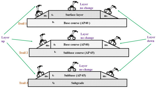
Figure 6.
Experiment setup in controlled experiments.

Table 1.
Considered variable values for data collection.
4.2. Data Collection in a Controlled Environment
In a controlled environment, sensors mounted on a UGV were run for all 54 scenarios to collect the dataset. Mainly, it consists of the three events of layer change (i.e., layer not changed, layer up and layer down), as shown in Figure 7. Then, these data were downloaded and transferred to the laptop after each sub-scenario. The subsequent manual labeling process was carried out according to the timestamp. In the collected data, the data points of each event were different, as sensors acquired data for each feature for the variant time. This imbalanced dataset of layer change features classes represents the real case. Random sampling was implemented to balance the data by augmenting the data of two feature classes (layer down and layer up), to avoid the biased classification result toward the dominating class. Consequently, the final number of data points of each feature class registered was 48,000.
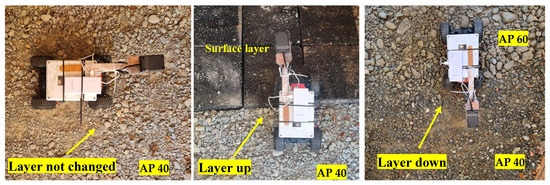
Figure 7.
Data collection in a controlled environment.
4.3. Implementation of Proposed Models
The deep learning model-based classifiers were developed using LSTM networks to detect the road layer change and classification. For that, acquired data were divided into training and testing datasets as 80% and 20% of the complete generated dataset in a controlled environment. Then, LSTM models were trained using a training dataset and tested on testing datasets to measure the deep learning performance. For that, Keras was used to build LSTMs classifiers, which provide TensorFlow to construct neural networks. Jupyter notebook was used to execute the LSTM model building process with Python 3.0. NVIDIA CUDA was utilized as a computing platform and API to allow software to use graphic processing units for general-purpose computing on GPU. The selected hyperparameters were selected during the implementation of models, as shown in Table 2. The window size was kept to 0.833 s after experimenting with various window sizes such as 0.66, 1.0, 1.2, and 1.4 s. The stochastic gradient as an optimizer minimizes the losses by helping the attributes to change in the model network, such as weights and learning rate. The regularization function supports the model robustness and minimizes the model complexity by adding the penalty to the loss function to eliminate the overfitting issues. Epochs define the total completed number of passes through the complete training dataset, which is delivered forward and backward through the neural network, whereas batch size refers to the sample number transmitted before the updating process of internal model parameters [37].
Table 2.
Hyperparameter information.
5. Result
5.1. Performance Result Comparison Models on Various Sensors Data
To examine the performance of proposed LSTMs models for various sensors combinations and determine the best sensor combination data, LSTMs models were constructed utilizing data of different sensor combinations, namely, (axyz + gxyz), (axyz + gxyz + D) and (az + gx + D). The performance measures were generated through the implementation of LSTMs on sensors combination. Figure 8 illustrates the comparison of overall accuracy, precision (P), recall (R), and F1 score for sensor combinations. The comparative result shows that the (az + gx + D) model obtained the highest accuracy as 97.88%, followed by (axyz + gxyz + D) through the ConvLSTM model. Furthermore, the LSTM implementation results of average precision, recall, and F1 score with the considered sensor combinations suggest that the combination of (az + gx + D) outperformed other sensor combinations in all model results. The model of acceleration + gyroscope performed poorly compared to (axyz + gxyz + D) and (az + gx + D) for all proposed algorithms.
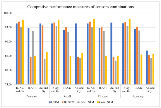
Figure 8.
Identification of best-performing sensor combination (az + gx + D) from the comparative result of all considered sensor combinations with LSTMs.
5.2. Classifier Results for (az + gx + D) Sensor Combination Data
According to the result of Section 5.1, it can be concluded that az + gx + D was the best sensor combination to classify road layer change events. Consequently, this section analyzes and compares the classification of road layer change classes results generated from using four implemented LSTM models for az + gx + D sensor data. This section consists of the precision, recall, and F1 score of each feature class and the overall accuracy, confusion matrix (CF), and accuracy–loss curve of each implemented model.
- (1)
- Figure 9 represents the confusion matrices of the proposed different LSTM models for az + gx + D sensor data. In a confusion matrix, the diagonal cells represent correctly identified events, and off-diagonal classes show misclassified events of specific layer classes. In the resultant confusion matrix of the proposed algorithms, X- and Y-axes depict the predicted and true classes. As shown in Figure 9, the proposed ConvLSTM outperformed the other LSTM networks with the fewest identification errors.
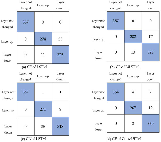 Figure 9. Confusion matrices of LSTMs.
 - (2)
- Model learning curves were plotted to examine the performance of models and obtain the bias–variance tradeoff [37]. Model learning curves illustrate the correlation between accuracy progress with epochs. Figure 10 and Figure 11 shows the recorded accuracy, loss for training, and validation datasets over the iterations for implemented LSTM models. These curves depict the tuning process of parameters with adjustment of the value to examine the accuracy and optimization loss of the considered validation dataset and training dataset. As observed from Figure 10 and Figure 11, the highest test accuracy and least test loss were obtained as 97.88% and 8.33%, respectively, for ConvLSTM. On the contrary, CNN-LSTM registered the lowest accuracy at 95.36% and the highest loss at 22.86%.
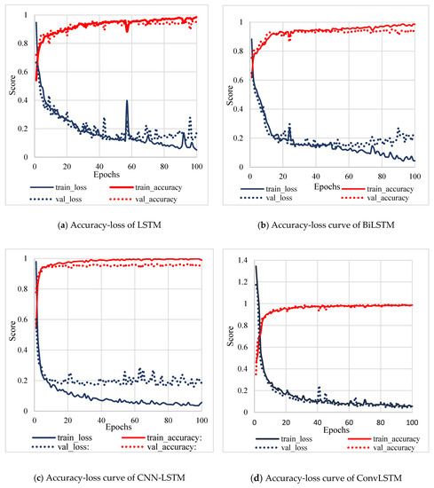 Figure 10. Model learning curves of LSTMs.
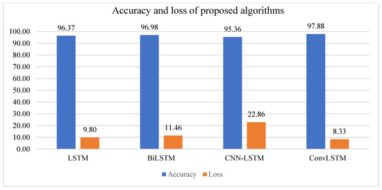 Figure 11. Accuracy and loss of proposed algorithm.
 - (3)
- Table 3 represents the precision, recall, and F1 score for each class of proposed algorithms. It can be observed from Table 1 that layer not changed received the highest precision at 100% with all LSTMs, whereas layer up attained the lowest precision at 88% with CNN-LSTM. Moreover, the highest recall value was observed for layer not changed at 100% with LSTM and BiLSTM, and the lowest recall value was registered for layer down at 90% with CNN-LSTM. Similarly, the highest F1 score was generated for layer not changed at 100 with LSTM, BiLSTM, and CNN-LSTM, and the lowest F1 score was evaluated for layer up at 92 with CNN-LSTM.
Table 3. Precision, Recall and F1 score.
6. Discussion
This study proposed a methodology for automated road layer change detection using LSTM algorithms from collected data through a sensor-equipped UGV. This research attempted to examine the capabilities of the sensors mounted UGV as an automated data collection technique and LSTM algorithms as automated data processing and analyzing techniques for automating the road layer change detection, which can lead toward automated road construction progress during the construction stage.
The common challenges of deep learning algorithms are the requirement of a large set of data and an imbalanced dataset, and these challenges were resolved by the data oversampling technique ‘random sampling’. This technique helped to achieve high training accuracy and robustness of the models. The results of the proposed study proved 0.833 s as the optimum window size according to the results of various experiments. First, this study examined the performance of three sensors combinations of (axyz + gxyz)), (axyz + gxyz +D) sensors, and (az + gx + D) to detect road layer change using LSTM, BiLSTM, CNN-LSTM, and ConvLSTM. The result of the study confirmed the (az + gx + D) sensor data as the best vector inputs and the (axyz + gxyz + D) combination as a satisfactory result, whereas the combination of accelerometer with gyroscope sensors underperformed following implementation with different LSTMs to achieve accuracy for the real-time road layer change classifications. This outcome implies that (az + gx + D) can efficiently classify road layer changes from collected data through the developed sensor prototype, which may potentially be used to measure as-built road progress. Further results were generated to examine the ability of LSTM implementation on (az + gx + D) sensor data to detect the layer changes. The consequent generated results suggest that ConvLSTM achieved the best accuracy of 97.88%, lowest loss of 8.33%, and minimization of overfitting issues for layer change classification compared to other implemented models. ConvLSTM showed great ability to predict spatiotemporal features of road layer change data using convolution structures which consist of state-to-state and input-to-state transitions. The presented convolutional in ConvLSTM aids in determining the future state of the certain grid according to the past states and inputs of the local neighbors. ConvLSTM is able to capture motions of UGV with transitional capture. Moreover, BiLSTM and LSTM also achieved good accuracy with a satisfactory fitting trend of learning curves, but CNN-LSTM showed an overfitting trend of learning curves. As observed from the learning curves of all proposed models, the values of validation loss and training loss converged for ConvLSTM, which indicates good model fitting on training and validation data. However, model learning curves illustrate a decrease in validation loss after 50 epochs for CNN-LSTM and BiLSTM. Overall, the implemented models obtained the desired accuracy. Nevertheless, the learning curves of the proposed models illustrated in Figure 10 depict that ConvLSTM predicted smoother classes with respect to ground-truth data, confirming it to be the superior model. In addition, the resultant high values of precision, recall, and F1 score of implemented models on sensor-collected data (az + gx + D) confirm the viability of the approach for real-time road layer change detection for as-built road progress measurement. The best performance for classifying the road layer change was detected for layers not changed with an accuracy of 100% with all LSTMs. In contrast, layer up achieved the lowest accuracy at 88% with CNN-LSTM. For layer up, ConvLSTM registered high values of precision (97%), recall (99%), and F1 (97%), whereas LSTM and BiLSTM achieved the highest precision, recall, and F1 score for layer not changed at 100%, 100%, and 100, respectively. It is also noted that CNN-LSTM received the highest precision for layer down as (97%), and ConvLSTM received the highest recall and F1 as 99% and 98, respectively. The obtained highest performance measures of layer not changed suggest the lowest errors when recognizing this class using the proposed approach.
Despite the promising performance of the models, the effect of the various hyperparameters was still obvious due to result variations according to various combinations of the parameters of algorithms such as classifier type, window size, neuron number, type of optimizer, regularizer type, and corresponding value. Finalizing the best parameter combinations of classifiers is a difficult task due to some reasons, such as variations in objectives behind road layer change detection on the same level implications, experimental protocol, type of attached sensor, and the nature of slope and thickness of the experiments. The use of sensor-armed unmanned ground vehicles showed great potential to recognize/detect road layers from collected data using distance, accelerometer, and gyroscope sensors in the control environment in this research. The result of performance measures depicts the improved robustness of the algorithm to fulfil the aim of automation in road progress monitoring. Road layer detection can be potentially carried out with layer change information and geometric design of road construction. The proposed approach will be potentially extended to the as-built measurement of pavement construction using the road layer change and spatial information (location of starting, ending, and change point) to calculate the as-built length of constructed road layers from their starting and finishing points.
7. Conclusions
An automated and real-time road layer detection framework for road construction enables a fundamental platform to assess and monitor pavement construction progress. This study explored the adoption of the low-cost sensor-equipped UGV to develop a road layer change classifier to detect the as-built road detection. In this study, the ToF ranging sensor, accelerometer, and gyroscope sensors were mounted on the UGV to record the sensor pattern data change for road layer change created in various scenarios created by changing the layers, thickness, and slope of layers. From this study, the random oversampling technique proved successful in data augmentation and data balancing to enhance the robustness of models. Subsequently, various deep learning algorithms, such as LSTM, BiLSTM, ConvLSTM, and CNN-LSTM, were implemented and compared for various combinations of sensors such as (az + gx + D), (axyz + gxyz + D), and (axyz + gxyz) to classify road layer change for automating the road layer changes detection process. The result proved az + gx + D as the best sensor combination with high-performance measures, followed by (axyz + gxyz + D). However, algorithms performed poorly on the combination of (axyz + gxyz), depicting the insufficiency of this sensor data combination to classify road layer change. Apparently, ConvLSTM stood out as the best-performing algorithm for (az + gx + D), with the highest overall accuracy at 97.88% and the lowest loss at 8.33%. Layer not changed obtained the highest value, whereas layer up and down achieved decent values of performance measures. The result of the study confirms the feasibility of the proposed classifier model with high-performance measures to predict layer change classes. This novel attempt confirms the potential successful application of the proposed sensor-equipped unmanned ground vehicle approach in road layer detection. This approach enables real-time automated monitoring solutions, which will relieve road construction companies from tedious and time-consuming manual methods.
8. Limitations and Future Study
This research is a stepping stone to automating pavement construction monitoring. However, it also had several limitations. The authors only considered 54 construction scenarios to develop a layer change classifier; however, more potential combinations of considered variables should be investigated with real cases. In this study, UGV-related variables were not considered, such as wheel size and various speeds of UGV. Further investigations can address this issue. This study was limited to developing a road layer classifier for the automated detection of road layer changes. However, this work should be extended to develop the complete approach of automated progress monitoring of road construction using sensors mounted on a UGV. Furthermore, automated navigation will be featured with UGV for planning data collection according to the schedule of activity and operation of machinery considering spatial conflicts.
Author Contributions
Conceptualization, T.P.; validation, T.P.; formal analysis, T.P.; investigation, T.P.; resources, T.P. and B.H.W.G.; data curation, T.P.; writing—original draft preparation, T.P.; writing—review and editing, T.P., B.H.W.G., J.D.v.d.W. and Y.Z.; visualization, T.P.; supervision, B.H.W.G., J.D.v.d.W. and Y.Z.; project administration, T.P. and B.H.W.G. All authors have read and agreed to the published version of the manuscript.
Funding
This research received no external funding.
Data Availability Statement
Data may be given on request. Please contact the corresponding author.
Conflicts of Interest
Authors declare no conflict of interest.
References
- Patel, T.D.; Haupt, T.C.; Bhatt, T. Fuzzy Probabilistic Approach for Risk Assessment of BOT Toll Roads in Indian Context. J. Eng. Des. Technol. 2020, 18, 251–269. [Google Scholar] [CrossRef]
- Vick, S.M.; Brilakis, I. A Review of Linear Transportation Construction Progress Monitoring Techniques. In Proceedings of the 16th International Conference on Computing in Civil and Building Engineering, ICCCBE2016, Osaka, Japan, 6–8 July 2016. [Google Scholar]
- Patel, T.; Guo, B.H.W.; Zou, Y. A Scientometric Review of Construction Progress Monitoring Studies. Eng. Constr. Archit. Manag. 2021, 29, 3237–3266. [Google Scholar] [CrossRef]
- Navon, R.; Shpatnitsky, Y. A Model for Automated Monitoring of Road Construction. Constr. Manag. Econ. 2005, 23, 941–951. [Google Scholar] [CrossRef]
- Del Pico, W.J. Project Control: Integrating Cost and Schedule in Construction; John Wiley & Sons: Hoboken, NJ, USA, 2013. [Google Scholar]
- Mubarek, S. Construction Project Scheduling and Control; John Wiley & Sons: Hoboken, NJ, USA, 2010. [Google Scholar]
- Golparvar-Fard, M.; Peña-Mora, F.; Savarese, S. Automated Progress Monitoring Using Unordered Daily Construction Photographs and IFC-Based Building Information Models. J. Comput. Civ. Eng. 2015, 29, 04014025. [Google Scholar] [CrossRef]
- Golparvar-Fard, M.; Peña-Mora, F.; Savarese, S. Monitoring Changes of 3D Building Elements from Unordered Photo Collections. In Proceedings of the IEEE International Conference on Computer Vision, Barcelona, Spain, 6–13 November 2011; pp. 249–256. [Google Scholar]
- Reja, V.K.; Varghese, K.; Ha, Q.P. Computer Vision-Based Construction Progress Monitoring. Autom. Constr. 2022, 138, 104245. [Google Scholar] [CrossRef]
- Rao, A.S.; Radanovic, M.; Liu, Y.; Hu, S.; Fang, Y.; Khoshelham, K.; Palaniswami, M.; Ngo, T. Real-Time Monitoring of Construction Sites: Sensors, Methods, and Applications. Autom. Constr. 2022, 136, 104099. [Google Scholar] [CrossRef]
- Khosrowpour, A.; Niebles, J.C.; Golparvar-Fard, M. Vision-Based Workface Assessment Using Depth Images for Activity Analysis of Interior Construction Operations. Autom. Constr. 2014, 48, 74–87. [Google Scholar] [CrossRef]
- Vick, S.; Brilakis, I. Road Design Layer Detection in Point Cloud Data for Construction Progress Monitoring. J. Comput. Civ. Eng. 2018, 32, 04018029. [Google Scholar] [CrossRef]
- Lo, Y.; Zhang, C.; Ye, Z.; Cui, C. Monitoring Road Base Course Construction Progress by Photogrammetry-Based 3D Reconstruction. Int. J. Constr. Manag. 2022, 1–15. [Google Scholar] [CrossRef]
- Golparvar-Fard, M.; Feniosky, P.M.; Savarese, S. D4AR-A 4-Dimensional Augmented Reality Model for Automating Construction Progress Monitoring Data Collection, Processing and Communication. Electron. J. Inf. Technol. Constr. 2009, 14, 129–153. [Google Scholar]
- Vick, S.M. Automated Spatial Progress Monitoring for Linear Transportation Projects. Ph.D. Thesis, University of Cambridge, Cambridge, UK, 2015. [Google Scholar]
- Kim, P.; Park, J.; Cho, Y.K.; Kang, J. UAV-Assisted Autonomous Mobile Robot Navigation for as-Is 3D Data Collection and Registration in Cluttered Environments. Autom. Constr. 2019, 106, 102918. [Google Scholar] [CrossRef]
- GAULD, L. Which Countries Have Banned Drones in 2022—The Silver Nomad. Available online: https://www.thesilvernomad.co.uk/countries-that-have-banned-drones/ (accessed on 10 November 2022).
- JIN, H. Where Are Drones Banned? Best Full Guide 2022—LucidCam. Available online: https://lucidcam.com/where-are-drones-banned/ (accessed on 10 October 2022).
- Malczan, N. Countries Where Drones Are Prohibited (Updated for 2022)—Droneblog. Available online: https://www.droneblog.com/countries-drones-prohibited/ (accessed on 11 October 2022).
- Hobby Henry 28 Countries That Have Banned Drones (UPDATED 2021)—Hobby Henry. Available online: https://hobbyhenry.com/countries-that-have-banned-drones/ (accessed on 11 October 2022).
- Sherafat, B.; Ahn, C.R.; Akhavian, R.; Behzadan, A.H.; Golparvar-Fard, M.; Kim, H.; Lee, Y.-C.; Rashidi, A.; Azar, E.R. Automated Methods for Activity Recognition of Construction Workers and Equipment: State-of-the-Art Review. J. Constr. Eng. Manag. 2020, 146, 03120002. [Google Scholar] [CrossRef]
- Joshua, L.; Varghese, K. Accelerometer-Based Activity Recognition in Construction. J. Comput. Civ. Eng. 2011, 25, 370–379. [Google Scholar] [CrossRef]
- Omar, T.; Nehdi, M.L. Automation in Construction Data Acquisition Technologies for Construction Progress Tracking. Autom. Constr. 2016, 70, 143–155. [Google Scholar] [CrossRef]
- Xu, Z.; Rao, Z.; Gan, V.J.L.; Ding, Y.; Wan, C.; Liu, X. Developing an Extended IFC Data Schema and Mesh Generation Framework for Finite Element Modeling. Adv. Civ. Eng. 2019, 2019, 1434093. [Google Scholar] [CrossRef]
- Civil Aviation Authority of New Zealand Drones—Aviation. Available online: https://www.aviation.govt.nz/drones/ (accessed on 10 November 2022).
- Nodari, F. 2022 Drone Regulations_ Where Can You Use It—Fabio Nodari. Available online: https://www.fabionodariphoto.com/en/drone-regulations-where-not-allowed-to-use/ (accessed on 10 November 2022).
- Asadi, K.; Kalkunte Suresh, A.; Ender, A.; Gotad, S.; Maniyar, S.; Anand, S.; Noghabaei, M.; Han, K.; Lobaton, E.; Wu, T. An Integrated UGV-UAV System for Construction Site Data Collection. Autom. Constr. 2020, 112, 103068. [Google Scholar] [CrossRef]
- Park, J.; Kim, P.; Cho, Y.K.; Kang, J. Framework for Automated Registration of UAV and UGV Point Clouds Using Local Features in Images. Autom. Constr. 2019, 98, 175–182. [Google Scholar] [CrossRef]
- Ryu, J.; Seo, J.; Jebelli, H.; Lee, S. Automated Action Recognition Using an Accelerometer-Embedded Wristband-Type Activity Tracker. J. Constr. Eng. Manag. 2019, 145, 04018114. [Google Scholar] [CrossRef]
- Kim, K.; Cho, Y.K. Effective Inertial Sensor Quantity and Locations on a Body for Deep Learning-Based Worker’s Motion Recognition. Autom. Constr. 2020, 113, 103126. [Google Scholar] [CrossRef]
- Rashid, K.M.; Louis, J. Times-Series Data Augmentation and Deep Learning for Construction Equipment Activity Recognition. Adv. Eng. Informatics 2019, 42, 100944. [Google Scholar] [CrossRef]
- Applied Technology Council. Field Manual: Post-Earthquake Safety Evaluation of Buildings; Applied Technology Council: Redwood City, CA, USA, 1989. [Google Scholar]
- Bosché, F. Automated Recognition of 3D CAD Model Objects in Laser Scans and Calculation of As-Built Dimensions for Dimensional Compliance Control in Construction. Adv. Eng. Informatics 2010, 24, 107–118. [Google Scholar] [CrossRef]
- Xu, Y.; Tuttas, S.; Hoegner, L.; Stilla, U. Voxel-Based Segmentation of 3D Point Clouds from Construction Sites Using a Probabilistic Connectivity Model. Pattern Recognit. Lett. 2018, 102, 67–74. [Google Scholar] [CrossRef]
- Patel, T.; Bapat, H.; Patel, D.; van der Walt, J.D. Identification of Critical Success Factors (CSFs) of BIM Software Selection: A Combined Approach of FCM and Fuzzy DEMATEL. Buildings 2021, 11, 311. [Google Scholar] [CrossRef]
- Golparvar-Fard, M.; Bohn, J.; Teizer, J.; Savarese, S.; Peña-Mora, F. Evaluation of Image-Based Modeling and Laser Scanning Accuracy for Emerging Automated Performance Monitoring Techniques. Autom. Constr. 2011, 20, 1143–1155. [Google Scholar] [CrossRef]
- Turkan, Y.; Bosche, F.; Haas, C.T.; Haas, R. Automated Progress Tracking Using 4D Schedule and 3D Sensing Technologies. Autom. Constr. 2012, 22, 414–421. [Google Scholar] [CrossRef]
- Bosché, F.; Ahmed, M.; Turkan, Y.; Haas, C.T.; Haas, R. The Value of Integrating Scan-to-BIM and Scan-vs-BIM Techniques for Construction Monitoring Using Laser Scanning and BIM: The Case of Cylindrical MEP Components. Autom. Constr. 2015, 49, 201–213. [Google Scholar] [CrossRef]
- Kang, L.-S.; Moon, H.S.; Dawood, N.; Kang, M.S. Development of Methodology and Virtual System for Optimised Simulation of Road Design Data. Autom. Constr. 2010, 19, 1000–1015. [Google Scholar] [CrossRef]
- Navon, R. Research in Automated Measurement of Project Performance Indicators. Autom. Constr. 2007, 16, 176–188. [Google Scholar] [CrossRef]
- Navon, R.; Goldschmidt, E. Monitoring Labor Inputs: Automated-Data-Collection Model and Enabling Technologies. Autom. Constr. 2003, 12, 185–199. [Google Scholar] [CrossRef]
- Costin, A.; Adibfar, A.; Hu, H.; Chen, S. Building Information Modeling (BIM) for Transportation Infrastructure—Literature Review, Applications, Challenges, and Recommendations. Autom. Constr. 2018, 94, 257–281. [Google Scholar] [CrossRef]
- GhasemiDarehnaei, Z.; Shokouhifar, M.; Yazdanjouei, H.; Fatemi, S.M.J.R. SI-EDTL Swarm Intelligence Ensemble Deep Transfer Learning for Multiple Vehicle Detection in UAVimages. Concurr. Comput. Pr. Exper. 2022, 34, e6726. [Google Scholar]
- Cezar, G. Activity Recognition in Construction Sites Using 3D Accelerometer Nd Gyroscope. 2018. Available online: https://www.semanticscholar.org/paper/Activity-Recognition-in-Construction-Sites-Using-3-Cezar/666162709fab34f211b71b5fee7fe1c781936aa2 (accessed on 10 November 2022).
- Akhavian, R.; Behzadan, A.H. Smartphone-Based Construction Workers’ Activity Recognition and Classification. Autom. Constr. 2016, 71, 198–209. [Google Scholar] [CrossRef]
- Bangaru, S.S.; Wang, C.; Busam, S.A.; Aghazadeh, F. ANN-Based Automated Scaffold Builder Activity Recognition through Wearable EMG and IMU Sensors. Autom. Constr. 2021, 126, 103653. [Google Scholar] [CrossRef]
- Yu, Y.; Si, X.; Hu, C.; Zhang, J. A Review of Recurrent Neural Networks: LSTM Cells and Network Architectures. Neural Comput. 2019, 31, 1235–1270. [Google Scholar] [CrossRef]
- Jamshed, A.; Mallick, B.; Kumar, P. Deep Learning-Based Sequential Pattern Mining for Progressive Database. Soft Comput. 2020, 24, 17233–17246. [Google Scholar] [CrossRef]
- Wang, K.; Zhao, W.; Cui, J.; Cui, Y.; Hu, J. A K-Anonymous Clustering Algorithm Based on the Analytic Hierarchy Process. J. Vis. Commun. Image Represent. 2019, 59, 76–83. [Google Scholar] [CrossRef]
- Wang, J.; Luo, Y.; Zhao, Y.; Le, J. A Survey on Privacy Preserving Data Mining. In Proceedings of the 2009 1st International Workshop on Database Technology and Applications, DBTA 2009, Wuhan, China, 25–26 April 2009; pp. 111–114. [Google Scholar]
- Slaton, T.; Hernandez, C.; Akhavian, R. Construction Activity Recognition with Convolutional Recurrent Networks. Autom. Constr. 2020, 113, 103138. [Google Scholar] [CrossRef]
- Hernandez, P.; Kenny, P. From Net Energy to Zero Energy Buildings: Defining Life Cycle Zero Energy Buildings (LC-ZEB). Energy Build. 2010, 42, 815–821. [Google Scholar] [CrossRef]
- Deng, W.; Li, Y.; Huang, K.; Wu, D.; Yang, C.; Gui, W. LSTMED: An Uneven Dynamic Process Monitoring Method Based on LSTM and Autoencoder Neural Network. Neural Netw. 2023, 158, 30–41. [Google Scholar] [CrossRef]
- Wang, J.; Chen, Y.; Hao, S.; Peng, X.; Hu, L. Deep Learning for Sensor-Based Activity Recognition: A Survey. Pattern Recognit. Lett. 2019, 119, 3–11. [Google Scholar] [CrossRef]
- Zhao, J.; Obonyo, E. Convolutional Long Short-Term Memory Model for Recognizing Construction Workers’ Postures from Wearable Inertial Measurement Units. Adv. Eng. Informatics 2020, 46, 101177. [Google Scholar] [CrossRef]
- Ilse, M.; Tomczak, J.M.; Forré, P. Selecting Data Augmentation for Simulating Interventions. Available online: http://proceedings.mlr.press/v139/ilse21a/ilse21a.pdf (accessed on 10 November 2022).
- Iwana, B.K.; Uchida, S. An Empirical Survey of Data Augmentation for Time Series Classification with Neural Networks. PLoS ONE 2021, 16, e0254841. [Google Scholar] [CrossRef] [PubMed]
- Wen, Q.; Sun, L.; Yang, F.; Song, X.; Gao, J.; Wang, X.; Xu, H. Time Series Data Augmentation for Deep Learning: A Survey. 2021, pp. 4653–4660. Available online: https://www.ijcai.org/proceedings/2021/0631.pdf (accessed on 10 November 2022).
- Minh Dang, L.; Min, K.; Wang, H.; Jalil Piran, M.; Hee Lee, C.; Moon, H. Sensor-Based and Vision-Based Human Activity Recognition: A Comprehensive Survey. Pattern Recognit. 2020, 108, 107561. [Google Scholar] [CrossRef]
- Li, Z.; Liu, Y.; Guo, X.; Zhang, J. Multi-ConvLSTM Neural Network for Sensor-Based Human Activity Recognition. J. Phys. Conf. Ser. 2020, 1682, 012062. [Google Scholar] [CrossRef]
- Farsi, M. Application of Ensemble RNN Deep Neural Network to the Fall Detection through IoT Environment. Alexandria Eng. J. 2021, 60, 199–211. [Google Scholar] [CrossRef]
- Li, F.; Shirahama, K.; Nisar, M.A.; Köping, L.; Grzegorzek, M. Comparison of Feature Learning Methods for Human Activity Recognition Using Wearable Sensors. Sensors 2018, 18, 679. [Google Scholar] [CrossRef]
- Kim, J.Y.; Cho, S.B. A Deep Neural Network Ensemble of Multimodal Signals for Classifying Excavator Operations. Neurocomputing 2022, 470, 290–299. [Google Scholar] [CrossRef]
- Ordóñez, F.J.; Roggen, D. Deep Convolutional and LSTM Recurrent Neural Networks for Multimodal Wearable Activity Recognition. Sensors 2016, 16, 115. [Google Scholar] [CrossRef]
- Antwi-Afari, M.F.; Qarout, Y.; Herzallah, R.; Anwer, S.; Umer, W.; Zhang, Y.; Manu, P. Deep Learning-Based Networks for Automated Recognition and Classification of Awkward Working Postures in Construction Using Wearable Insole Sensor Data. Autom. Constr. 2022, 136, 104181. [Google Scholar] [CrossRef]
- Murugesan, R.; Mishra, E.; Krishnan, A.H. Deep Learning Based Models: Basic LSTM, Bi LSTM, Stacked LSTM, CNN LSTM and Conv LSTM to Forecast Agricultural Commodities Prices. Int. J. Sustain. Agric. Manag. Informatics 2021, 8, 242–277. [Google Scholar]
- Cao, Y.; Ashuri, B. Predicting the Volatility of Highway Construction Cost Index Using Long Short-Term Memory. J. Manag. Eng. 2020, 36, 04020020. [Google Scholar] [CrossRef]
- Amer, F.; Golparvar-Fard, M. Automatic Understanding of Construction Schedules: Part-of-Activity Tagging. Proc. 2019 Eur. Conf. Comput. Constr. 2019, 1, 190–197. [Google Scholar] [CrossRef]
- Goyal, A.; Gupta, V.; Kumar, M. A Deep Learning-Based Bilingual Hindi and Punjabi Named Entity Recognition System Using Enhanced Word Embeddings. Knowledge-Based Syst. 2021, 234, 107601. [Google Scholar] [CrossRef]
- Moradzadeh, A.; Teimourzadeh, H.; Mohammadi-Ivatloo, B.; Pourhossein, K. Hybrid CNN-LSTM Approaches for Identification of Type and Locations of Transmission Line Faults. Int. J. Electr. Power Energy Syst. 2022, 135, 107563. [Google Scholar] [CrossRef]
- Shi, X.; Chen, Z.; Wang, H.; Yeung, D.Y.; Wong, W.K.; Woo, W.C. Convolutional LSTM Network: A Machine Learning Approach for Precipitation Nowcasting. Adv. Neural Inf. Process. Syst. 2015, 2015, 802–810. [Google Scholar]
- Khan, N.; Haq, I.U.; Ullah, F.U.M.; Khan, S.U.; Lee, M.Y. Cl-Net: Convlstm-Based Hybrid Architecture for Batteries’ State of Health and Power Consumption Forecasting. Mathematics 2021, 9, 3326. [Google Scholar] [CrossRef]
- Géron, A. Hands-on Machine Learning with Scikit-Learn and TensorFlow: Concepts, Tools, and Techniques to Build Intelligent Systems; O’Reilly Media, Inc.: Sebastopol, CA, USA, 2017; ISBN 9781491962299. [Google Scholar]


Disclaimer/Publisher’s Note: The statements, opinions and data contained in all publications are solely those of the individual author(s) and contributor(s) and not of MDPI and/or the editor(s). MDPI and/or the editor(s) disclaim responsibility for any injury to people or property resulting from any ideas, methods, instructions or products referred to in the content. |
© 2022 by the authors. Licensee MDPI, Basel, Switzerland. This article is an open access article distributed under the terms and conditions of the Creative Commons Attribution (CC BY) license (https://creativecommons.org/licenses/by/4.0/).