Article

Estimation of Soil–Structure Model Parameters for the Millikan Library Building Using a Sequential Bayesian Finite Element Model Updating Technique

1
Department of Civil and Environmental Engineering, University of Nevada, Reno, NV 89577, USA
2
Department of Civil and Environmental Engineering, University of California, Los Angeles, CA 90095, USA
3
Department of Mechanical and Civil Engineering, California Institute of Technology, Pasadena, CA 91125, USA
*
Author to whom correspondence should be addressed.
Buildings 2023, 13(1), 28; https://doi.org/10.3390/buildings13010028
Submission received: 20 November 2022 / Revised: 14 December 2022 / Accepted: 15 December 2022 / Published: 22 December 2022

Abstract

:
We present a finite element model updating technique for soil–structure system identification of the Millikan Library building using the seismic data recorded during the 2002 Yorba Linda earthquake. A detailed finite element (FE) model of the Millikan Library building is developed in OpenSees and updated using a sequential Bayesian estimation approach for joint parameter and input identification. A two-step system identification approach is devised. First, the fixed-base structural model is updated to estimate the structural model parameters (including effective elastic modulus of structural components, distributed floor mass, and Rayleigh damping parameters) and some uncertain components of the foundation-level motion. Then, the identified structural model is used for soil–structure model updating wherein the Rayleigh damping parameters, the stiffness and viscosity of the soil subsystem (modeled using a substructure approach), and the foundation input motions (FIMs) are estimated. The identified model parameters are compared with state-of-practice recommendations. While a specific application is made for the Millikan Library, the present work offers a framework for integrating large-scale FE models with measurement data for model inversion. By utilizing this framework for different civil structures and earthquake records, key structural model parameters can be estimated from the real-world recorded data, which can subsequently be used for assessing and improving, as necessary, state-of-the-art seismic analysis and structural modeling techniques. This paper presents an effort towards using real-world measurements for large-scale FE model updating in the soil and structure, uniform soil time domain for joint parameter and input estimation, and thus paves the way for future applications in system identification, health monitoring, and diagnosis of civil structures.

1. Introduction

The dynamic response of a building structure to an earthquake excitation is occasionally the result of a complex interaction between the structural system and the underlying and surrounding geology. Since modeling the physics of a coupled soil–structure system in detail is an intricate undertaking, the state of practice has adopted simplified modeling and analysis procedures, such as the substructure approach (e.g., [1,2]). In this approach, the soil flexibility and energy dissipation are modeled using distributed spring and dashpot elements to which the foundation input motions (FIMs) are applied as uniform base excitations [3]. The stiffness and viscosity of these elements are derived using simplified analytical methods, which are nonetheless based on idealized and restrictive assumptions—e.g., linear elastic response behavior of soil and structure, uniform soil half-space (or soil profiles with stiffness gradually varying with depth [4]), etc. These simplifying assumptions and the empirical nature of the mechanical analogs (e.g., soil springs and dashpots) could potentially lead to unquantified errors in predicting the seismic responses of real-world building structures, even though the simplified models have demonstrated acceptable accuracy in idealized case studies (e.g., [5]). Furthermore, integrating the substructure method with the Rayleigh damping model—which itself has a highly empirical nature—introduces another source of uncertainty in the seismic analysis of building structures. Clearly, there is an inconsistency between the relatively sophisticated mechanics-based techniques available for structural system modeling and the crude simplicity of the underlying assumptions that guide the damping and soil–structure interaction (SSI) models. It appears clear that the efforts on damping and SSI characterization should be guided by observations distilled from real-life data.
Soil–structure interaction (SSI) analysis has been an active research subject for more than 40 years (e.g., [6]). SSI effects can be classified into two categories: kinematic and inertial interaction effects [7]. Referred to as the FIMs, the earthquake excitations experienced by a structure–foundation system are affected by the stiffness contrast between the foundation stiffness and the surrounding geology. Therefore, FIMs are generally different from the Free-Field Motions (FFMs) that would have been recorded in the absence of the foundation system. The effects of foundation stiffness and geometry, which result in discrepancies between FIMs and FFMs, are collectively referred to as the kinematic interaction effects. Inertial interaction effects are a result of the foundation–superstructure mass, which imparts inertial forces onto the surrounding soil and causes the foundation to experience a response different from the FIMs. Due to the inertial interaction effects, the vibrating structure operates as a wave source and alters the wave field around the foundation system. In the substructure modeling approach, these two effects are treated separately (e.g., [8]). That is, FIMs are analytically or numerically calculated based on the soil and foundation properties (e.g., [9]). Then, inertial effects are represented by frequency-dependent impedance functions that are estimated through analytical, numerical, or experimental studies (e.g., [10]). Finally, the superstructure on top of the impedance functions is analyzed under the estimated FIMs.
In this study, we develop a model inversion framework that can be used to back-calculate the soil–structure model parameters from the seismic responses of real-world buildings. By repeating this effort for different buildings and earthquake records, the estimation results can be summarized and compared with the state-of-practice recommendations to improve the present seismic analysis capabilities and predictive models for building structures. We apply the model inversion framework that is devised in the present study to the data recorded from the Millikan Library building during the 2002 Yorba Linda earthquake, which was a low-amplitude seismic event. The response of the building during this small event was nearly linear elastic. As such, it provides an opportunity to compare the estimation results with linear elastic seismic analysis practices.
The utilized model inversion framework is based on a finite element (FE) model updating approach formulated in the time domain, using a sequential Bayesian estimation method [11]. The FE model updating approach has been developed and verified previously using numerically simulated data (e.g., [12,13]). This paper presents an effort towards using real-world measurements for large-scale FE model updating in the time domain, and thus paves the way for future applications. Although the presented model updating approach is used along with a linear FE model in this study, the approach can be readily extended to nonlinear FE models of civil structures.
In what follows, the Bayesian FE model updating approach and its algorithmic details are briefly discussed in Section 2. Section 3 provides the modeling details of the Millikan Library building. A two-step system identification approach is introduced in Section 4, which is applied to the Millikan Library data in Section 5 and Section 6. An identifiability analysis accompanies each system identification step to select the estimation parameters. Finally, the key estimation results are summarized and compared with available literature and the state of practice in Section 7.

2. Data Assimilation through FE Model Updating in the Time Domain

The finite element model of a building structure depends on various “model parameters”. Model parameters include, but are not limited to, inertial properties, damping parameters, parameters that characterize the stiffness properties of the structural and nonstructural components, and the time histories of the unmeasured components of base excitation. If the soil–structure interaction effects are included in the FE model, then the parameters used to model the soil subsystem and the time history of FIMs are also unmeasurable and unknown. Using the recorded acceleration response time histories of the building during an earthquake, our objective is to identify the best estimates of the unknown model parameters along with the input excitation time history, in order to minimize the discrepancy between the FE-predicted and measured structural responses.
The estimation problem is tackled by updating iteratively and sequentially the joint probability distribution function (PDF) of the unknown model parameters and the discrete values of the input motion time histories using a Bayesian inference method. The basics of the sequential FE model updating method for joint system and input identification are presented in [11]. Here, we briefly review the technical background of this method and highlight the new improvements introduced for this study.

2.1. Bayesian FE Model Updating in Time Domain for Joint System and Input Identification

The predicted response of a FE model at time step i to an earthquake excitation time history can be expressed as [14]
y ^ i = h i ( θ , u ¨ 1 : i g )
where y ^ i n y × 1 denotes the vector of structural response quantities predicted by the FE model at time step i (i = 1, 2, …, k), θ n θ × 1 denotes the FE model parameter vector, u ¨ i g n u ¨ × 1 denotes the vector of unknown or unmeasured input ground motion at time step i, n u ¨ denotes the number of unknown or unmeasured input ground motion components, and u ¨ 1 : i g = [ ( u ¨ 1 g ) T ( u ¨ 2 g ) T ( u ¨ i g ) T ] T is the vector of the unknown or unmeasured input ground motion time history. h i ( ) is the response function of the FE model at time step i, which, in general, is a nonlinear function of θ and u ¨ 1 : i g . The measured response vector of the structure, y i , is related to the FE-predicted response, y ^ i , as ([12,13,14])
v i ( θ , u ¨ 1 : i g ) = y i y ^ i
where v i n y × 1 is the simulation error vector, which accounts for the misfit between the measured and FE-predicted responses. This misfit stems from the output measurement noise, parameter uncertainties, and model errors. Model errors stem from simplifying idealizations adopted when devising the model as well as deviations in its geometry and configuration from the real-life structure it represents, which result in an inherent discrepancy between the FE model prediction and the measured structural responses [15].
Given an unbiased estimate of θ and u ¨ 1 : k g , it is assumed here that the simulation error can be modeled as a stationary, zero-mean, and independent Gaussian white noise process [16]. Therefore, the likelihood function can be derived as
p ( y i | θ , u ¨ 1 : i g ) = p ( v i ) = 1 ( 2 π ) n y / 2 | R | 1 / 2 e 1 2 v i T R 1 v i   = 1 ( 2 π ) n y / 2 | R | 1 / 2 e 1 2 ( y i h i ( θ , u ¨ 1 : i g ) ) T R 1 ( y i h i ( θ , u ¨ 1 : i g ) ) T
where | R | denotes the determinant of the diagonal matrix R n y × n y , which is the time-invariant covariance matrix of the simulation error vector, i.e., R = E ( v i v i T ) , i . The unknown model parameter vector and time histories of the unknown input ground motion can be stacked into an extended unknown parameter vector defined as ψ = [ θ T , ( u ¨ 1 : k g ) T ] T . In a stochastic model inversion, the uncertainty in the unknown parameter vector is characterized by a joint probability distribution function (PDF). The objective in FE model updating is to find an estimate of the unknown parameters such that their joint posterior PDF given the measured output response of the structure is maximized. This is referred to as the maximum a posteriori (MAP) estimate. Using Bayes’ rule, it can be observed that
( ψ ^ ) MAP = arg max ψ   p ( ψ   |   y 1 : k ) = arg max ψ   p ( y 1 : k   |   ψ ) × p ( ψ )
where p ( y 1 : k   |   ψ ) = i = 1 k p ( v i ) , and p ( ψ ) is the joint prior PDF of the extended unknown parameters.

2.2. Sequential Finite Element Model Updating Using Model Linearization

Solving the MAP estimation problem shown in Equation (4) using a batch optimization algorithm can be computationally demanding [11]. Therefore, a sequential estimation approach is introduced in [11] to improve the computational efficiency and convergence rate. In this approach, the estimation time domain is divided into successive overlapping time windows, referred to as the estimation windows. The estimation problem is solved iteratively at each estimation window to estimate the posterior mean vector and covariance matrix of the unknown parameters. At each iteration, the FE model is linearized to propagate the uncertainties in the prior PDF into the FE model response. The posterior mean vector and covariance matrix of the unknown parameter vector are then derived using Equation (4), and used as prior information for the next iteration. Once the iterations converge for an estimation window, the estimated mean vector and covariance matrix are transferred to the next estimation window and are used as prior information. In what follows, the mathematical process of the sequential Bayesian estimation approach is outlined.
Assume that the mth estimation window with length t l spans from time step t 1 m to time step t 2 m , where t l = t 2 m t 1 m . Considering that p ( y t 1 m : t 2 m   | ψ m ) = i = t 1 m t 2 m p ( v i ) , and assuming a Gaussian distribution for the joint prior PDF, the natural logarithm of the posterior joint PDF of the extended unknown parameter vector, i.e., ψ m = [ θ T , ( u ¨ t 1 m : t 2 m g ) T ] T , can be derived as [11]
l o g ( p ( ψ m   |   y t 1 m : t 2 m ) ) = k 0 1 2 ( y t 1 m : t 2 m h t 1 m : t 2 m ( ψ m , u ¨ ^ 1 : t 1 m 1 g ) ) T R ˜ 1 ( y t 1 m : t 2 m h t 1 m : t 2 m ( ψ m , u ¨ ^ 1 : t 1 m 1 g ) ) 1 2 ( ψ m ψ ^ m ) T ( P ^ ψ , m ) 1 ( ψ m ψ ^ m )
where k 0 is a constant, and ψ ^ m and P ^ ψ , m are the prior mean vector and the covariance matrix of the extended parameter vector at the mth estimation window. R ˜ ( t l × n y ) × ( t l × n y ) is a block diagonal matrix, in which the diagonals denote the simulation error covariance matrix R , and u ¨ ^ 1 : t 1 m 1 g is the estimated input motion time history from the previous estimation windows, which is treated as a known vector. To determine the MAP estimate of ψ m , we solve l o g ( p ( ψ m   |   y t 1 m : t 2 m ) ) ψ m = 0 , which results in a nonlinear algebraic equation in ψ m , as shown in [11]. This equation can be solved using an iterative first-order approximation of the FE response function at ψ ^ m , which requires the computation of FE response sensitivities with respect to the extended unknown parameter vector, evaluated at the prior mean values. The FE response sensitivity matrix is denoted by C hereafter. As a result, the following (first-order approximate) equation for the MAP estimate of ψ m can be obtained [11] as
ψ ^ m , j + = ψ ^ m , j + K ( y t 1 m : t 2 m h t 1 m : t 2 m ( ψ ^ m , j , u ¨ ^ 1 : t 1 m 1 g ) )
where ψ ^ m + is the updated (or the posterior) mean estimate of ψ m . The term K = P ^ ψ y ( P ^ y y ) 1 is referred to as the Kalman gain matrix [17]. The matrix P ^ ψ y = P ^ ψ , m C T is the cross-covariance matrix of the unknown parameter vector and measured data, and P ^ y y = C P ^ ψ , m C T + R ˜ is the covariance matrix of the measured data (the reader is referred to [11,18] for further derivation details). The subscript j is appended to the estimated mean vector and covariance matrix to denote the iteration number. The updated ψ ^ m , j + from Equation (6) is iteratively used as the new point for the linearization of the nonlinear FE model to improve the estimation. This iterative prediction–correction procedure at each estimation window is equivalent to an iterative extended Kalman filtering (EKF) method for parameter-only estimation [17]. Following the EKF procedure, the prior covariance matrix P ^ ψ , m , j is updated to the posterior covariance matrix P ^ ψ , m , j + at each prediction–correction iteration as in
P ^ ψ , m , j + = ( I K C ) P ^ ψ , m , j ( I K C ) T + K R ˜ K T .
Furthermore, to improve the convergence characteristics of the iterative prediction–correction procedure, a disturbance matrix is added to the posterior covariance matrix at each iteration to provide the prior covariance matrix for the next iteration, i.e., P ^ ψ , m , j + 1 = P ^ ψ , m , j + + Q , in which Q is a diagonal matrix with small positive diagonal entries (relative to the diagonal entries of the matrix P ^ ψ , m , j + ). The matrix Q is referred to as the process noise covariance matrix in the Kalman filtering world [17].
Accurately computing the FE response sensitivities is an integral part of the presented sequential FE model updating. In previous studies (e.g., [11,12]), the response sensitivities have been computed using a direct differentiation method (DDM) (e.g., [19]), which requires extending the FE numerical scheme and implementing new codes in the FE software to calculate the response sensitivities. Although available in OpenSees [20], this implementation is not readily available as part of other FE simulation platforms. Therefore, to extend the applicability of the sequential FE model updating procedure to other FE simulation platforms, here we use the finite difference method (FDM) to compute the response sensitivities. The FDM method is implemented by perturbing the estimation parameters one at a time based on a central difference method with unequal spacing. We use parallel computing to enhance the computational efficiency of the FDM implementation. The Bayesian FE model updating algorithms are implemented in MATLAB [21], which calls several instances of OpenSees in parallel for FE response and response sensitivity computations at each prediction–correction iteration. Table 1 summarizes the sequential FE model updating algorithm for the joint estimation of model parameters and input motion time histories that is described above. It should be noted that the presented Bayesian FE model updating framework is applicable to both linear and nonlinear FE models. In case the FE model is linear, the model response function will still be a nonlinear function of the model parameters and input motion; however, the model updating process will become more computationally efficient.

2.3. Correction for Constraints

The estimation process described earlier is not constrained and may result in the estimation of non-physical values for the model parameters. This issue is resolved by correcting the posterior estimation results for a set of predefined lower- and upper-bound constraints. Once any of the posterior mean values exceed their designated lower or upper limit, the posterior Gaussian PDF (characterized by the updated mean vector and covariance matrix) is truncated at the constraint edges. The mean vector and the covariance matrix of the truncated PDF are then calculated. The constraint correction approach is borrowed from [17,22]. The algorithmic details are provided in [23] and are not repeated here for brevity.

2.4. Adaptive Scaling of the Unknown Model Parameters

In order to improve the performance of the estimation algorithm, the FE model parameters are scaled adaptively at each iteration. The scaling allows the FE model responses to have relatively similar sensitivities with respect to different estimation parameters at each estimation point. The scaled FE model parameter vector is defined as θ s = A θ , in which A is an n θ × n θ diagonal scaling matrix. It should be noted that only the FE model parameters are scaled, and the vector of unknown input ground motion remains unscaled. The parameter scaling factors (i.e., the diagonal entries of matrix A denoted by a n , n = 1 , 2 ,   , n θ ) are calculated to result in equal corresponding diagonal entries in the Fisher Information Matrix of the scaled parameters, which is approximated as I s = ( C θ s ) T ( C θ s ) [14], wherein C θ s denotes the FE response sensitivity matrix with respect to the scaled FE model parameter vector. The nth diagonal entry of I s is I n s = 1 a n 2 ( h θ n ) T ( h θ n ) . The scaling factor a n is calculated so that I n s is equal to the mean of diagonal entries of the Fisher Information Matrix corresponding to the vector of unknown input ground motion, i.e., for the mth estimation window:
1 a n 2 ( h θ n ) T ( h θ n ) = m e a n [ d i a g ( ( h u ¨ t 1 m : t 2 m g ) T ( h u ¨ t 1 m : t 2 m g ) ) ] a n   = ( h θ n ) T ( h θ n ) m e a n [ d i a g ( ( h u ¨ t 1 m : t 2 m g ) T ( h u ¨ t 1 m : t 2 m g ) ) ]

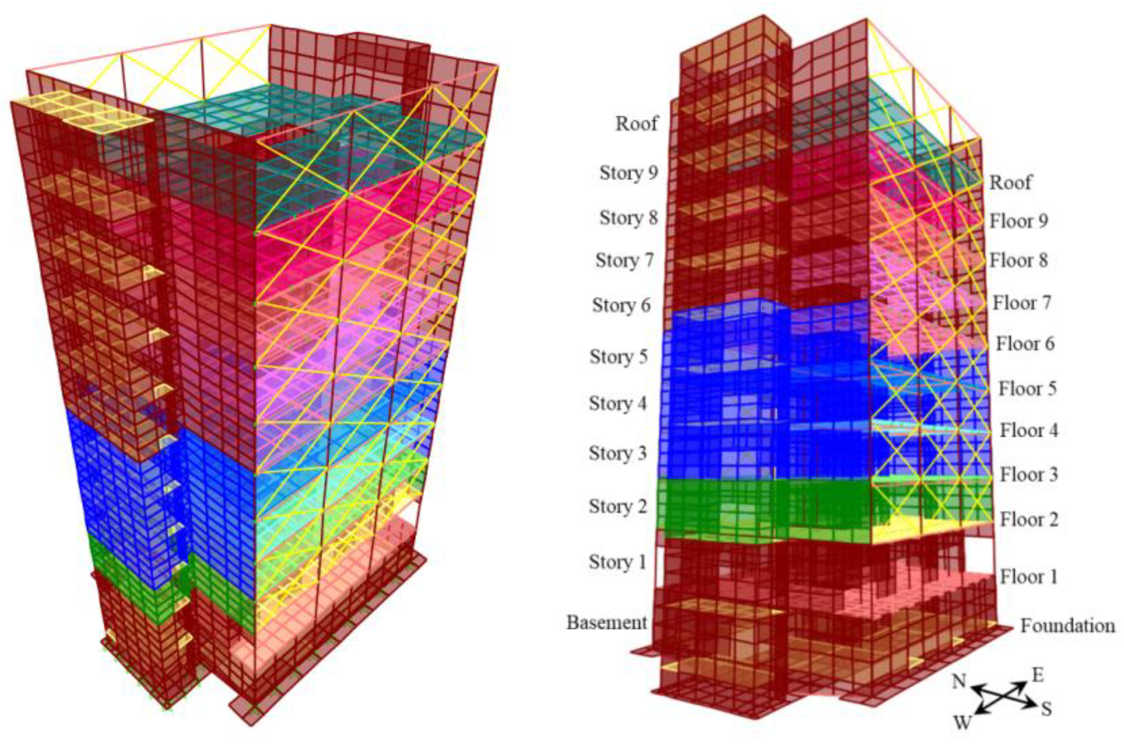
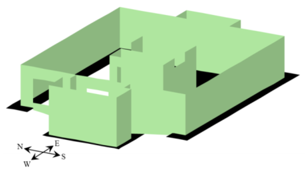
3. The Millikan Library Building

The Millikan Library is a reinforced concrete shear wall building, with a basement and nine stories above the ground, located on the California Institute of Technology (Caltech) campus (Figure 1). The Millikan Library has been the subject of many studies, especially in the fields of soil–structure system identification, due to its unique structural and soil properties, and its relatively old and dense instrumentation, which recorded its seismic responses during numerous earthquakes [24,25,26,27,28,29,30]. The Millikan Library building is 43.9 m tall above ground, including the roof level. It has a 4.3 m deep basement below the ground level. The basement is encased by surrounding shear walls. Precast concrete claddings are installed on the north and south faces of the building from the second floor up to the roof. The lateral force-resisting system comprises shear walls in the north–south direction on the east and west sides of the building and core walls around the elevator shaft in the north–south and east–west directions. The floor system consists of concrete slabs supported by reinforced concrete beams. Lightweight aggregate concrete is used for slabs and beams at all floors, while regular aggregate concrete is used for foundations, columns, and walls. The foundation system consists of a 1.2 m deep central pad, 6.0 m below the ground level, and two foundation strips on the north and south sides of the building 5.0 m below the ground level. Four stepped beams at the four corners of the foundation connect the central foundation pad to the north and south foundation strips.
The building is instrumented using a total of 36 uniaxial accelerometers, measuring six acceleration responses at the foundation (or basement floor) level, and three translational acceleration responses on each floor. The instrumentation details are obtained from [31] and are provided in Figure A1 and Table A1 in Appendix A. Multiple earthquake records are available for the Millikan Library; a relatively recent survey of earthquake data recorded at the building can be found in [28]. For the purpose of this study, we use the 2002 Yorba Linda earthquake record, which is a low-amplitude earthquake (PGA of ~0.6% g). Two notes should be made about this earthquake record of the Millikan Library. First, the location of sensors on the foundation (or basement floor) could not be determined precisely. Second, recordings of the east sensor on the second and eighth floors (measuring NS direction) were not available during the 2002 Yorba Linda Earthquake. Therefore, only 34 measurement channels are available for this record. Since the level of considered earthquakes is low, the effects of material and geometric nonlinearities in the dynamic response of the structure are expected to be minor, and therefore, the use of a linear model is justified.

FE Model Development

Using the available structural drawings, a detailed FE model of the structural system was developed. We used the graphical user interface of SAP2000 software [32] to develop the initial geometry of the model. The SAP2000 model was then transferred to OpenSees [20] using a custom-developed MATLAB script based on the SAP2000 Application Programming Interface (API). For the purpose of this study, we prepared a linear FE model of the Millikan Library building. The model comprises linear elastic beam–column elements for the buildings’ beams and columns, and quadrilateral shell (DKGQ) elements with linear elastic (elastic membrane plate) sections are used for shear walls and slabs. The kinematic interaction of precast claddings (installed on the north and south faces of the building) with the structural system is modeled using diagonal brace elements, which are included in the north and south frame bays from the second story to the roof. The brace elements are assumed to be linear elastic with square cross-sections of 0.1 m × 0.1 m. By adjusting the elastic modulus of the diagonal braces, the stiffness and force contributions of the precast panels to the lateral response of the structure can be characterized. The kinematic interaction between the structure and other nonstructural components and systems (e.g., partition walls and stairs) are not modeled explicitly; they are expected to be lumped into the stiffness properties of the structural members and precast claddings.
The inertial effects of nonstructural components (i.e., stairs, precast panels, and elevators) are accounted for by modeling their corresponding mass and weight contributions. The weight of each precast panel is estimated to be about 50 kN, which conforms with [24]. A uniformly distributed load is applied on the floor slabs to account for live loads and weight of partition walls, later treated as an unknown parameter to be estimated. A uniformly distributed load of 2.5 kN/m2 is applied on the foundation to account for the live load of library shelves in the basement. Moreover, the mass of soil filling between the foundation surface and basement floor is accounted for by applying the corresponding mass on the central foundation pad and the two foundation strips. The mass of structural components is calculated based on the nominal concrete densities specified in the structural drawings: ρ c L W = 1760 kg m 3 for lightweight aggregate concrete material, ρ R C L W = 1900 kg m 3 for lightweight aggregate reinforced concrete, and ρ R C = 2500 kg m 3 for regular aggregate reinforced concrete. Figure 2 shows the geometry of the model. Different colors in this figure present different material property groups used to define the shell (shear wall and slab) and beam–column elements. More details on material parameters are provided in Section 5. A sensitivity analysis is performed to ensure convergence of analysis results with respect to the mesh size. The model in the presented configuration consists of 1885 frame elements and 4043 shell elements, corresponding to a total of 27,526 degrees of freedom.
A gravity analysis was performed before dynamic time history analyses by applying constant g acceleration in the vertical direction. The damping energy dissipation for the time history analysis is defined using mass- and stiffness-proportional Rayleigh damping. The Rayleigh damping parameters are treated as unknowns to be estimated. For the purpose of time history analyses, Newmark’s constant average acceleration method is used for time-stepping with increments of Δ t = 0.03   s . The time step size is selected following a convergence study to ensure a large time step size that provides adequate accuracy. All of the measured acceleration response time histories are also resampled at Δ t = 0.03   s for the model updating phase.

4. A Two-Step System Identification Approach

A two-step FE model updating approach is used for model and input identification of the soil–structure system. In the first step, the measured acceleration responses at the foundation level are used to calculate six components of the foundation-level motions. The foundation-level motions are then used as uniform base input excitations, and the measured responses of the structure are used as output measurements to update the FE model of the “fixed-base” structure. The objective is to estimate the model parameters characterizing the structural model, regardless of the soil subsystem. During this process, we discovered inconsistencies in the recordings obtained from two of the foundation sensors, as is discussed further in the next section. These sensors are installed inside a utility tunnel—referred to as the steam tunnel—next to the foundation slab. Therefore, the acceleration response time histories of these two sensors are assumed as unknown input motions and are estimated jointly with the structural model parameters. This step results in FE model updating with partially unknown inputs.
The second step is an output-only FE model updating procedure, wherein the identified structural model parameters are fixed at their mean estimates obtained from the first step, and the three translational components of FIM and other parameters characterizing the soil–structure model are estimated jointly. Since the Millikan Library foundation is not deep and does not have large dimensions (comparable with the lengths of incident waves), the rotational components of FIM are not considered in this study.
To decide about and select the estimation parameters, an identifiability analysis is performed, as is outlined in the next section for each identification step. Before proceeding with the real-life data, we verified the two-step FE model updating procedure using numerically simulated data to examine the effectiveness of the proposed estimation algorithm and the accuracy of its results. The verification studies are documented in [33] and are not included here for brevity.

5. Step 1 System Identification: FE Model Updating of the Structural System with Partially Unknown Inputs

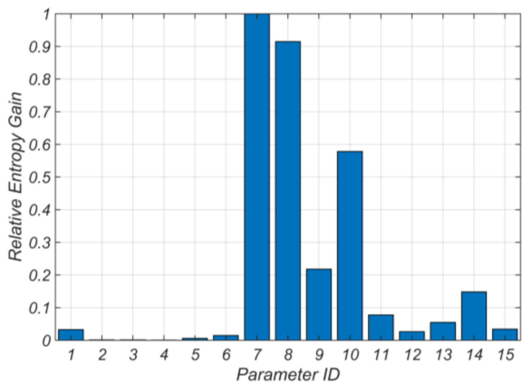
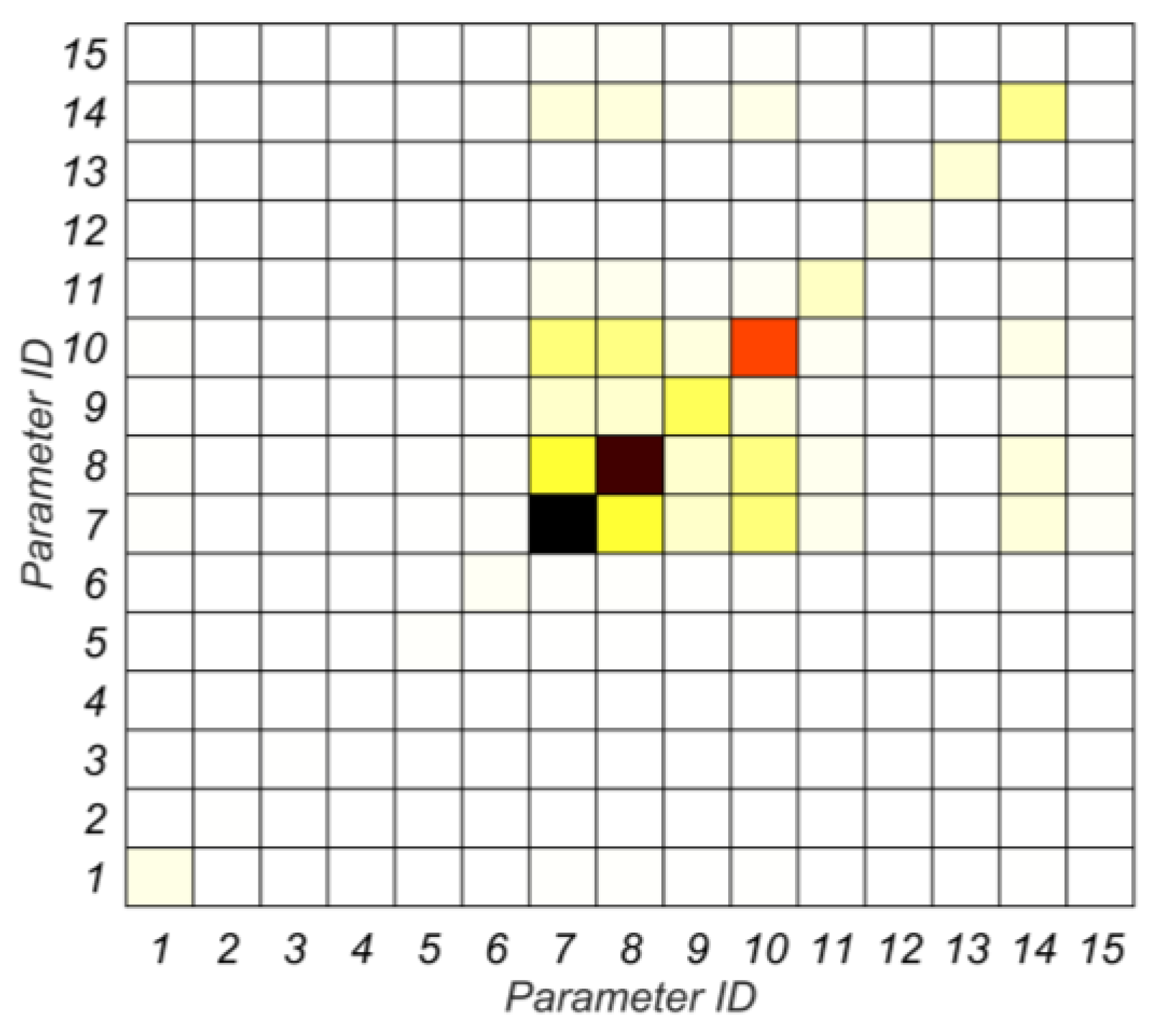
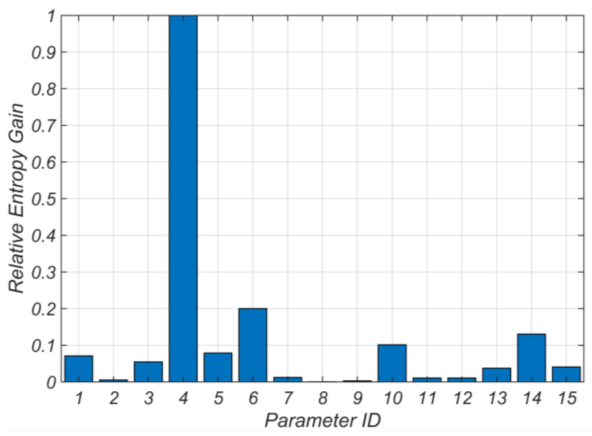
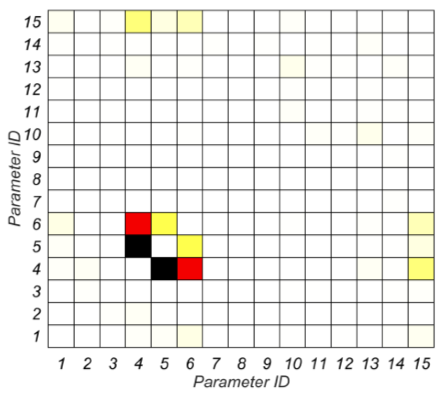
5.1. Model Identifiability and Parameter Selection

The identifiability of model parameters is investigated using an information-theoretic approach based on [34]. In this approach, a set of candidate parameters are selected first, and then, the entropy gain of each parameter is calculated. The entropy gain is used as a quantitative metric to measure the information each model parameter receives from the measurement data. The entropy gain is compared between the estimation parameters to assess their relative identifiability. Moreover, the mutual entropy gain (or mutual gain) between parameter pairs is used to investigate the dependence between each pair of model parameters. The entropy gain and mutual gain are then used to determine the most identifiable parameter set. This is an alternative procedure to prior methods that, for example, adaptively group updating parameters based on the sensitivities of a model updating objective function with respect to the parameters (e.g., see [35,36]).
Fifteen (15) structural model parameters characterizing the material, inertial, and damping properties were initially selected as the estimation parameters for identifiability assessment at this step. These parameters were selected initially based on our judgment on their potential contribution in the structural response. For a given input motion, the entropy gain for each parameter is a function of the parameter values, which are unknown in advance. Without the knowledge of correct parameter values, their nominal values are used for prior identifiability assessment, following the recommendation in [34]. These parameters and their nominal values are listed in Table 2. The logic based on which the nominal values are estimated is further described below.
The material parameters consist of the effective elastic modulus of the floor system (beams and slabs) and the vertical/lateral system (walls and columns). The material parameters are grouped at the story level and along the height of the building. With the exception of the first three stories, the effective elastic modulus of structural components is grouped together at the upper stories. The first three stories are considered separately because previous studies have suggested minor structural damage in the first stories of the building after the 1971 San Fernando earthquake (e.g., [26,37,38]). The effective elastic modulus for floor slabs and beams is calculated by applying a 35% reduction factor on the nominal elastic modulus of lightweight aggregate concrete, which is derived based on ACI 318-14 [39] as E c = 0.043 ( ρ c L W ) 1.5 f c , where f c = 27.5   MPa is the nominal compressive strength. The effective elastic modulus for columns and walls is calculated by applying a 70% reduction factor on the nominal elastic modulus calculated as E c = 4700 f c , where f c = 27.5   MPa . For foundation, a 35% reduction factor is applied on the elastic modulus, which is calculated considering f c = 20.7   MPa , to account for flexural cracking.
To estimate the elastic modulus of diagonal brace elements representing the precast claddings, the results concluded from modal analysis performed during the construction period are used. According to [6,26], the installation of precast panels resulted in a 25% increase in the lateral stiffness of the building structure in the EW direction. The initial values for the elastic modulus of the diagonal brace elements in the model are tuned iteratively and manually to yield a similar increase in the stiffness of the first mode in the EW direction. Consequently, the estimated elastic modulus of diagonal braces is found to be 20 GPa. The initial value of the distributed floor mass (to account for live load and mass of nonstructural elements) is estimated to be about 250 kg/m2. Estimating the accurate weight and mass contribution of mechanical equipment on the roof was not possible; therefore, the equivalent distributed roof mass is approximately estimated as 300 kg/m2. Finally, the initial values of the Rayleigh damping parameters are estimated by assuming a 5% damping ratio for the first and second modes.
The identifiability of model parameters is assessed using the measured foundation-level motion, including all translational and rotational components. As mentioned earlier, the recordings of two acceleration channels on the foundation are later treated as unknowns and estimated through the model updating process. Nevertheless, these measured recordings are used for the identifiability analysis as approximate inputs. This approximation is expected to have negligible effects on the overall identifiability results. As described in [34], evaluating the entropy gain and mutual gain also requires the prior covariance matrix of the unknown parameter vector (or the prior variance of parameters). A 10% coefficient of variation is assumed for all parameters to derive the a priori covariance matrix.
Figure 3 displays the relative entropy gain of the fifteen candidate estimation parameters. The presented entropy gains are relative, which means that the entropy gain values are scaled with respect to the largest value. This plot presents the relative information that the model responses (which represent the measurements) carry about each model parameter. Those parameters that receive small information from the measurement data (e.g., parameters #2 to #6) are likely to be unidentifiable. Furthermore, Figure 4 shows the relative mutual entropy gain between the parameter pairs. This figure is used to investigate the dependence between each two parameters. The diagonal components in this figure represent the entropy gain of each parameter. The dark off-diagonal colors in this figure indicate strong relative dependence between parameter pairs. For example, Figure 4 suggests that there is a mutual dependence between parameters #7 and #8, and some mutual dependence between parameters #7, #8, and #10. Moreover, there are some competing effects between these parameters and parameter #14. These observations are physically meaningful since parameters #7, #8, and #10 characterize the stiffness of the building, and parameter #14 contributes to the building mass. Figure 3 along with Figure 4 can be used to guide the selection of the estimation parameters. The parameters that gain relatively small amounts of information from the measurement data or have strong dependencies on other estimation parameters can be put aside (i.e., fixed) or merged with other parameters, if physically meaningful, to enhance the identifiability. Indeed, the process is not definitive and requires some engineering judgment in selecting the final estimation parameter set.
The strong mutual gain between parameters #7 and #8 suggests merging these two parameters into a single unknown parameter. This is justifiable as these parameters characterize the effective elastic modulus of columns and walls at the basement level and the first story, which are expected to be close. The mutual gains between other stiffness-related parameters are not significant; nevertheless, their small entropy gains in Figure 3 suggest merging them together. Furthermore, since the initial estimate of mass-related parameters (#14 and #15) are close and their individual entropy gains are small, they are also merged together to improve their identifiability. Finally, while the entropy gains of parameters #1 and #12 are small, we still consider them as unknown parameters to be estimated; however, the resulting estimates are expected to be inaccurate and include large uncertainties. As a result of the outlined identifiability assessment process, we end up with six estimation parameters, as listed in Table 3.

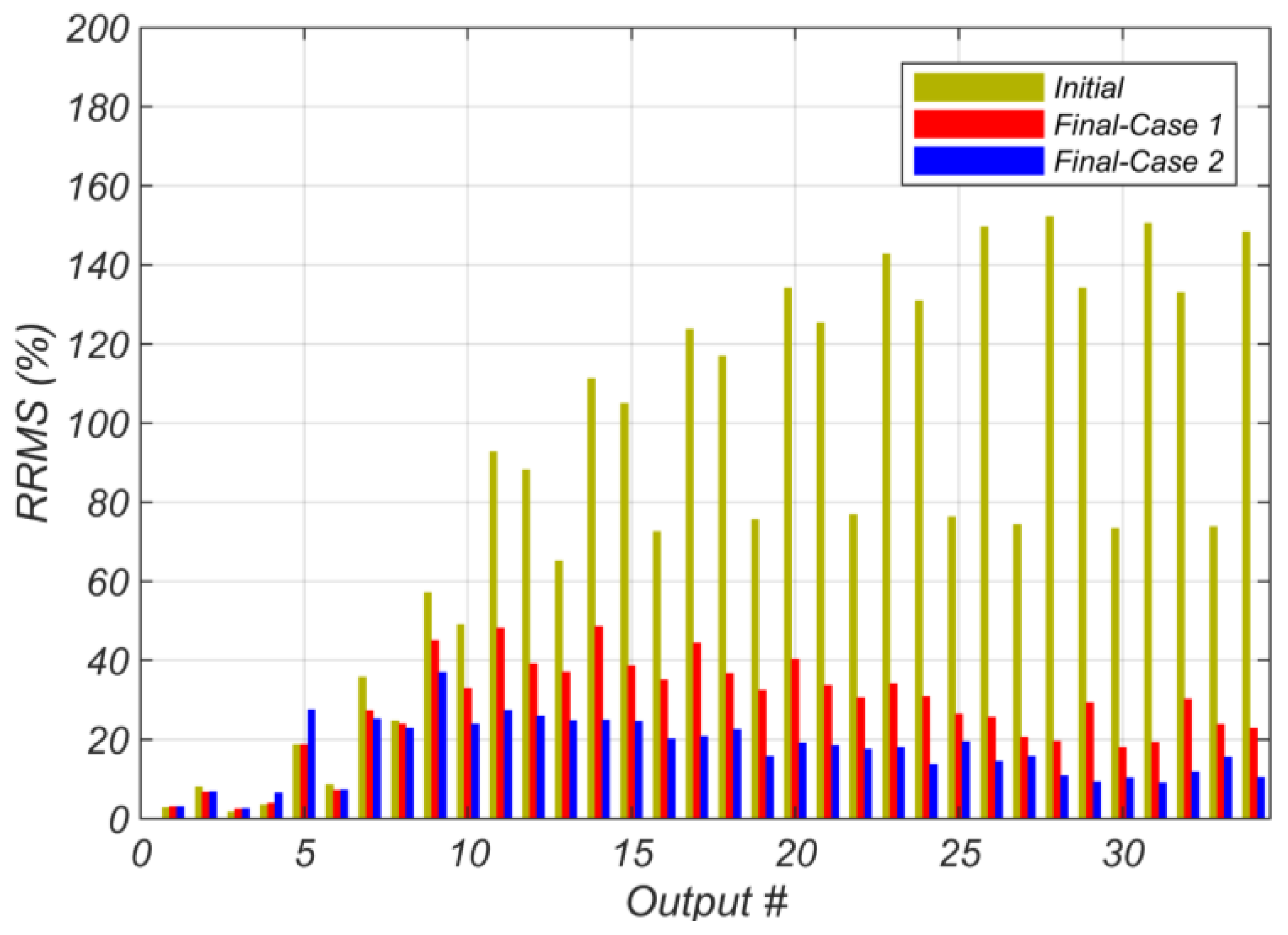
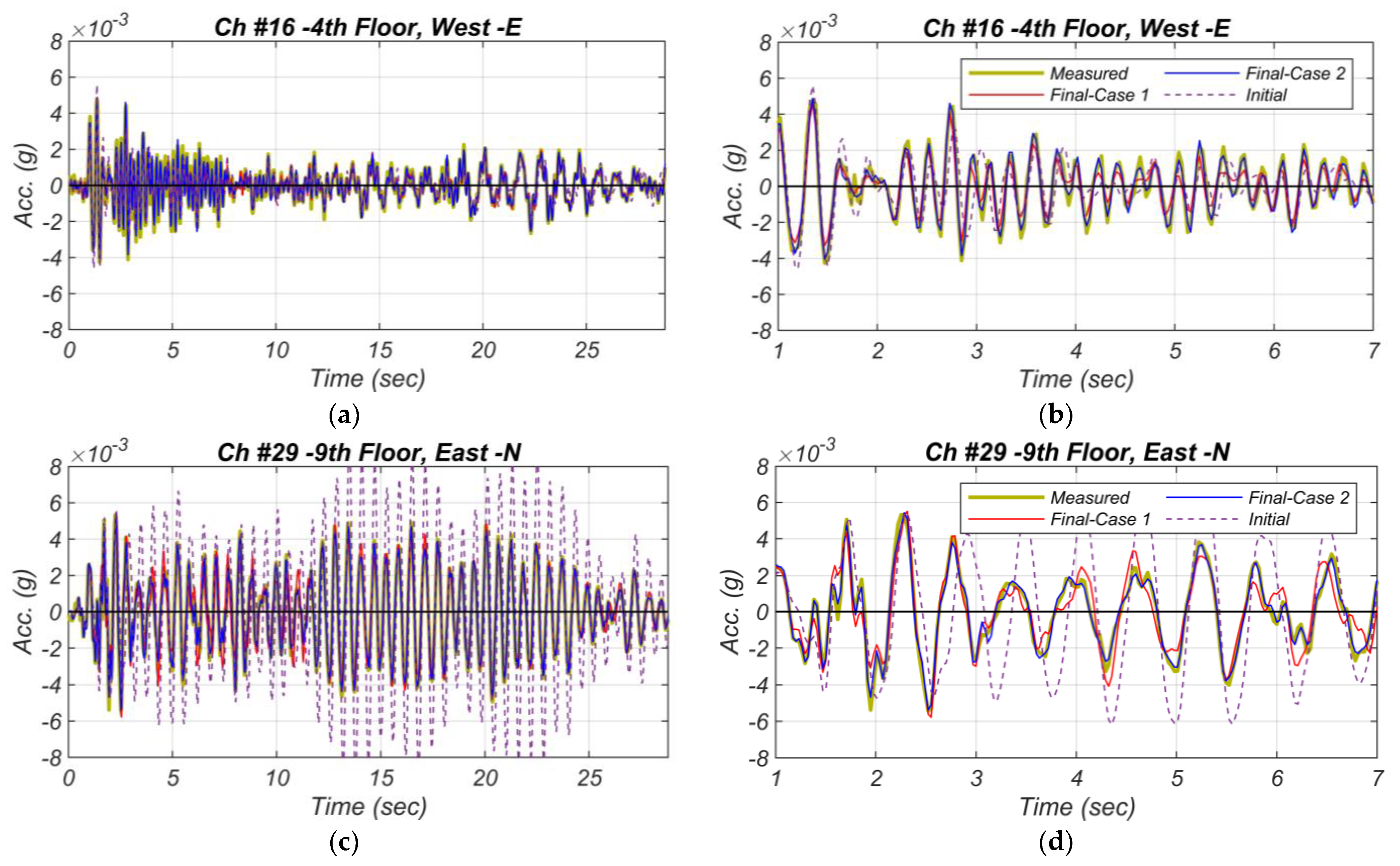
5.2. Joint System and Partial Input Identification Using Yorba Linda Earthquake Data

The seismic data recorded at the Millikan Library building during the 2002 Yorba Linda earthquake are utilized for the FE model updating. Here, we present two model updating cases. In Case 1, the recordings of the six accelerometers installed on the foundation are averaged to find the time histories of translational and rotational components of the foundation-level motion. These input excitations along with the measured structural responses obtained from all the channels are used for an “input–output” FE model updating to estimate the six model parameters listed in Table 3. In Case 2, we assume that the recordings of the two sensors located in the steam tunnel, i.e., Channels #4 and #5, are unknown. This resulted in FE model updating with partially unknown inputs to jointly estimate the six model parameters and the acceleration response time history at two sensor locations.
Figure 5 presents the relative root mean square error (RRMSE) between the measured and FE predicted acceleration responses for both Case 1 and Case 2. The figure also shows the RRMSE values obtained from the initial FE model (i.e., based on the initial parameter values). As can be seen in this figure, the RRMSE is consistently reduced from the initial to the updated FE model in both cases. However, Case 2 shows more reduction in RRMSE for all measurement channels compared to Case 1 except for Channels #4 and #5, in which RRMSEs are increased. This suggests that these two sensor measurements do not comply with the other measurements on the foundation level. Hence, the updated FE model in Case 2 is most likely a better representation of the real-world building. As shown in Appendix A, these two channels correspond to the sensors installed in the steam tunnel—Channel #4 measures the acceleration response in the NS-direction and Channel #5 in the Up–Down or Z-direction. The steam tunnel is a rectangular reinforced concrete utility access tunnel built next to the foundation level and is not part of the basement structure. After the 1971 San Fernando Earthquake, a 0.5 mm crack around the steam tunnel, at the point where the tunnel connects to the basement wall, was reported [37]. Based on these observations, it is concluded that the tunnel is most likely not fully connected to the structural system, and thus, the readings of the accelerometers located in there may not correctly represent the foundation level motions. Figure 6 compares the measured and estimated acceleration response time histories at Channels #4 and #5. The differences between the measured and estimated acceleration time histories are minor and more prominent for Channel #5, which is the Z-direction measurement.
The initial and final estimates of the six model parameters, along with their final estimated coefficients of variation (COVs), are listed in Table 4. The coefficient of variation quantifies the estimation uncertainty. In an unbiased estimation, the COV should merge to zero. The non-zero values for the COV mean that the estimation might be uncertain. The larger the COV, the more uncertainty there is in the estimated model parameter values. As can be seen in Table 4, the COV of the two parameters with the highest COV in case 1, i.e., EClad and m, is significantly reduced in Case 2. It is also seen that the estimate of these parameters is unrealistically low in Case 1, while their estimates in Case 2 seem to be more realistic. These results, along with the RRMSE results shown in Figure 5, indicate that Case 2 is likely to be more reliable than Case 1, and hence, the parameter estimates from this case will be used for the next step.
Figure 7 shows how well the updated model predictions match the measurement records for both model updating cases, wherein selected measured acceleration response time histories are shown together with those estimated using the initial and final updated FE models. The figure shows that while the initial FE model response predictions have remarkable discrepancies with the measured responses, the updated model predictions have good agreement with the measurements. It also shows that the updated model predictions in Case 2 have better agreement with the measurements than Case 1, which further proves the reliability of Case 2 over Case 1. In the next paragraph, we describe the details of the estimation algorithm setup.
The initial values of model parameters ( θ ^ 0 ) are listed in Table 3, and their initial coefficient of variation is selected as 10%. The estimation constraints for model parameters are selected as 0.1 θ ^ 0 θ 5 θ ^ 0 . The initial estimate of the discrete values of the unknown ground motion time history is selected to be zero, and their initial standard deviation is selected as 0.05 Rad s 2 . A variable estimation window configuration (length and overlap) is considered. During the first 6 s of the earthquake (which corresponds to the strong motion part), a small window length (60 time steps = 1.8 s) with 50% overlap is used. As we march through the time history, the estimation window length is gradually increased to 100 time steps (3 s) with 20% overlap. Selecting smaller lengths and larger overlaps for the estimation windows at the beginning of the earthquake ensures the incremental absorption of the information when the model has large uncertainties and the measurements have large information content (due to strong motion). The window length is subsequently increased and the overlap is reduced to improve the computational efficiency. The estimation window configuration can affect the computation demand and the estimation accuracy and should be selected based on experience and adjusted by observing the performance of the estimation algorithm.
The process noise covariance matrix Q (see Table 1) is selected as a diagonal matrix. The diagonal entry corresponding to the ith model parameter is selected as ( q θ ^ i ) 2 , where q = 0.001 and θ ^ i is the mean estimate of the ith model parameter. This means that the RMS of the process noise corresponding to the model parameters is taken as 0.1% of the mean estimate of the associated model parameter. Thus, this part of the matrix Q would be time-varying. The diagonal entries corresponding to the unknown ground motion time histories are constant, and are taken as (0.001g)2. This means that the root mean square (RMS) of the process noise corresponding to the input excitation is time-invariant and is equal to 0.1% g. This selection is performed based on our previous experience with the estimation algorithm to ensure stability and proper convergence rate (more discussions are provided in [11]). Finally, the simulation error covariance matrix R is also selected as a time-invariant diagonal matrix, whose diagonal entries are selected as (0.001g)2. In other words, the simulation error is modeled as a 0.1% g RMS Gaussian white noise process.

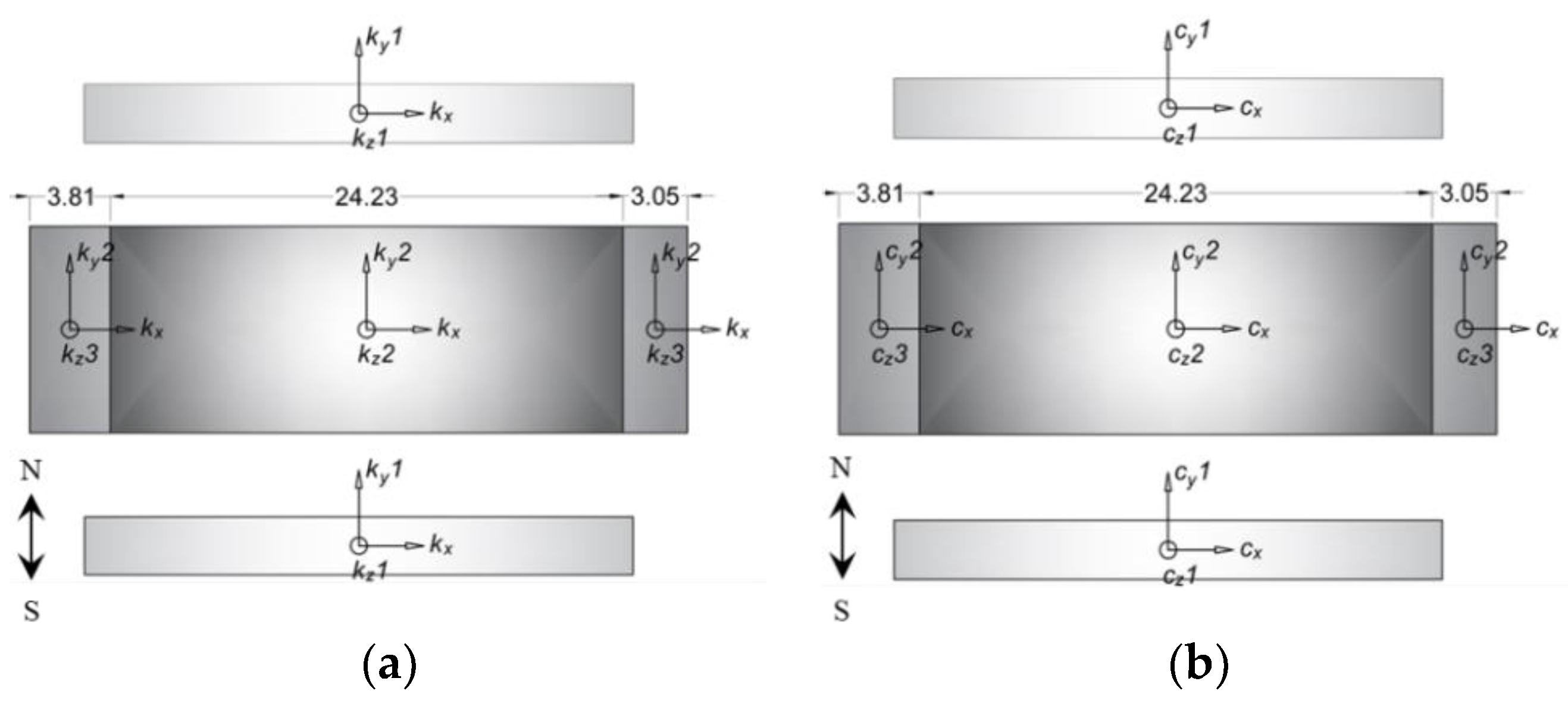
6. Step 2 System Identification: FE Model Updating of the Soil–Structure System with Unknown Inputs

At this stage, we use the updated model of the superstructure (Case 2) for soil–structure system identification. The objective is to estimate the FIMs and the parameter characterizing the soil–structure system, including the stiffness and viscosity of the soil springs and dashpots used for modeling the inertial soil–structure interaction effects. For this purpose, and similar to the previous step, we start with an identifiability analysis by evaluating the information contained in the model responses. Then, we use the real measurement data to estimate the soil–structure model parameters.

6.1. Model Identifiability and Parameter Selection

Distributed linear soil springs and dashpots are included underneath the foundation slab of the updated FE model, obtained from the previous step. Three linear springs and three linear viscous dashpots are modeled independently in the x-, y-, and z-direction (corresponding to EW, NS, and Up–Down directions, respectively) at each nodal point of the foundation slab. The stiffness of soil springs and viscosity of dashpots are computed using the subgrade modulus (i.e., soil stiffness per unit area) and viscosity modulus (i.e., soil viscosity per unit area), respectively. The spring stiffness and dashpot viscosity at each nodal point are calculated by multiplying the tributary area of the nodal point by the corresponding subgrade modulus and viscosity modulus, respectively.
The Millikan Library has a two-level foundation system consisting of a central pad and two north and south foundation strips, as shown in Figure 8. Six unknown subgrade moduli—namely kx, ky1, ky2, kz1, kz2, and kz3—are defined for different foundation regions, where, for example, the parameter kz2 characterizes the vertical subgrade modulus for the interior area of the central pad. Two strips along the east and west edges of the central pad, which are underneath the two box shear walls at the east and west sides of the building, are assigned a different vertical subgrade modulus (kz3) based on the recommendation provided in [3] to account for the rotational stiffness of the soil subsystem. Similarly, a different vertical subgrade modulus (kz1) is assigned to the two north and south foundation strips. Likewise, six (unknown) parameters—namely cx, cy1, cy2, cz1, cz2, and cz3—are used to define the viscosity modulus. Different foundation regions and their corresponding subgrade and viscosity modulus are shown in Figure 9. The twelve unknown subgrade and viscosity moduli along with the Rayleigh damping parameters (α and β) and the effective elastic modulus of foundation slabs (EFound) are selected as parameters for the identifiability analysis. Although estimated in the previous step, the Rayleigh damping parameters are included for the soil–structure system identification since the damping model behavior of the fixed-based structure is expected to be different from the flexible-base structure.
To assess the identifiability of these fifteen (15) unknown parameters, we pursue the same identifiability analysis approach presented before. Initial estimates of soil model parameters are assigned using the NIST standard guidelines [3]. The FIMs are unknown at this stage and will be estimated through the model updating process. In the absence of the correct FIMs, the three translational components of the foundation-level motion, estimated from the previous step, are used as the FIMs for identifiability assessment. The parameters used for identifiability analysis and their corresponding initial values are listed in Table 5. The initial values of the Rayleigh damping parameters are selected based on the estimation results obtained in the previous step. Moreover, a 20% coefficient of variation is assumed for all parameters to derive the a priori covariance matrix.
Figure 10 displays the relative entropy gain of the fifteen estimation parameter candidates. Figure 11 displays the mutual entropy gain between parameter pairs. In Figure 11, the diagonal terms (i.e., entropy gain of estimation parameters) are found to be much larger than the off-diagonal terms (i.e., mutual entropy gain between parameter pairs); hence, including both of them in the figure would underrepresent the off-diagonal terms since they would appear with a hard-to-see, light color. Therefore, the diagonal terms are excluded from this figure. These two figures can be used together for selecting the estimation parameters. Figure 10 shows that some of the parameters (e.g., parameters #2, #8, #11, and #12) receive little information from the measurements. These parameters are, therefore, unlikely to be identifiable. Based on this figure, parameters #2 and #3, which represent the subgrade modulus in the north direction for the foundation beams and central pad, respectively, are merged together. This is due to the small relative entropy gain of parameter #2. Similarly, parameters #8 and #9, and #10 to #12 are merged together to improve their identifiability. Moreover, Figure 11 shows mutual dependence between parameter #15 and parameters #4 to #6. This implies that the estimation of the effective elastic modulus of foundation slabs will likely affect the estimation accuracy of the vertical and rocking soil stiffnesses. Hence, parameter #15 is fixed at its nominal value given the relatively large thickness of foundation slab, which is expected to result in linear elastic behavior. Based on this identifiability study, the estimation parameters characterizing the soil–structure model are reduced to ten, which are kx, ky, kz1, kz2, kz3, cx, cy, cz, α, and β.

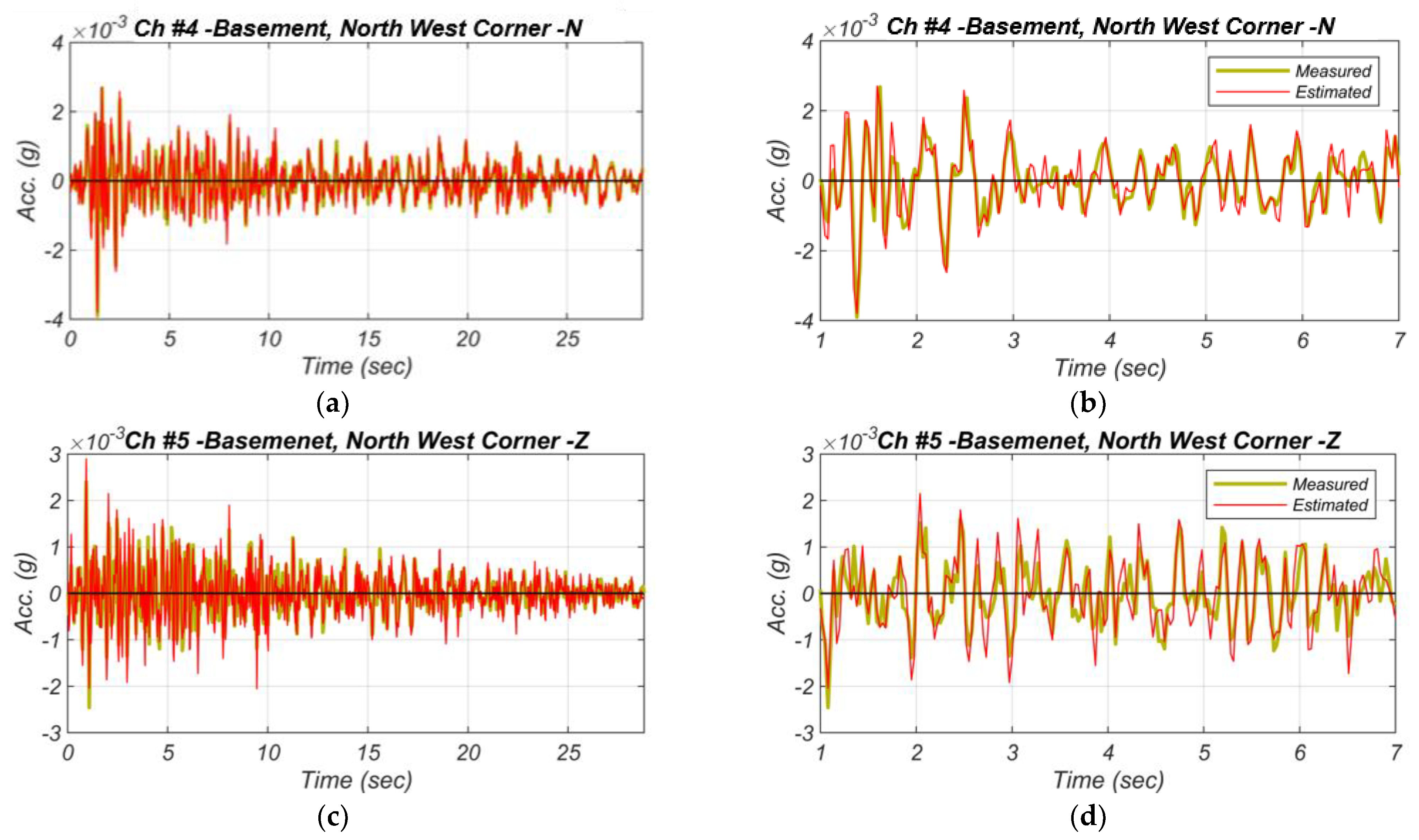
6.2. Joint System and Input Identification Using the Recorded Yorba Linda Earthquake Data

The seismic data recorded at the Millikan Library building during the 2002 Yorba Linda earthquake are now utilized in an output-only FE model updating procedure to estimate the eight soil parameters, two Rayleigh damping parameters, and the three components of the FIM in EW, NS, and Up–Down directions (no rotational component is considered for the FIM). The model parameters characterizing the superstructure (except the Rayleigh damping parameters) are kept constant based on the estimated results obtained from the previous system identification step. Except the initial coefficient of variation of estimation parameters, which is selected as 20%, and the estimation constraints for model parameters, which are selected as 0.01 θ ^ 0 θ 50 θ ^ 0 , the setup of the estimation algorithm and its parameters are similar to the previous step (see Section 5.2).
Figure 12 shows the time history of the posterior mean and standard deviation (SD) of the three components of the FIM. The initial and final estimates of the ten soil–structure model parameters along with the estimated coefficient of variation (COV) are listed in Table 6. The estimated parameter values with larger COV include larger estimation uncertainties. Figure 13 compares the measured acceleration response time histories at the selected measurement channels with those estimated using the final estimates of the model parameters and FIMs. This figure indicates that there is a remarkable agreement between the estimated and measured acceleration responses. Furthermore, Figure 14 presents the RRMSE of the updated FE model responses at different measurement channels. Comparing Figure 14 with Figure 5, the discrepancies between the FE predictions and measurements in the NS direction are generally less than those in the EW direction. This is predictable since the soil–structure interaction effects are more dominant in the NS direction of the Millikan Library [28], and hence, the flexible-base model uncertainty is expected to be less in the NS direction than in the EW direction.

7. Summary and Discussion

7.1. Effective Structural Stiffness Parameters

The estimated effective elastic moduli of columns and walls (EW&C1 = 19.6 GPa, EW&C2 = 26.1 GPa) are larger than the nominal value that is based on code recommendations, which is 17.3 GPa. Several factors can collectively account for this difference. (i) The effects of lateral stiffness of the backfill soil at the basement level are not modeled in the FE model. This is likely the reason behind the larger estimated value for EW&C1. It can also be a source of modeling error because the columns and walls at the first-story and basement level are parameterized with the same effective elastic modulus. (ii) Concrete aging, which will increase the stiffness of concrete material, is not accounted for in the nominal estimations. (iii) The lateral stiffness of nonstructural components and systems (i.e., partition walls and stairs) are not accounted for in the FE model. This can result in estimating larger values for the effective elastic moduli of the columns and walls, which characterize the lateral stiffness of the building. (iv) Finally, the nominal elastic modulus is calculated for the concrete material without accounting for the effects of steel reinforcement, which can partially explain the larger estimated effective elastic moduli.

7.2. Soil Subsystem Stiffness and Viscosity

Table 7 compares the estimated lumped stiffness and viscosity of the soil subsystem with the NIST recommendations [3] based on [40]. The lumped soil stiffness and viscosity should be evaluated at the fundamental frequency of soil–structure system using the flexible-base dimensionless frequency a 0 = ω ˜ b V s , where ω ˜ is the flexible-base fundamental circular frequency, b = 11.5 m is the foundation half-width, and V s is the shear wave velocity, which is averaged over an effective soil profile depth based on the recommendations provided in [3]. Using the shear wave velocity profile of the Millikan Library site presented in [41], the average shear wave velocity is calculated as 398.1 m/s for translation, 392.1 m/s for rocking in the NS direction, 407.7 m/s for rocking in the EW direction, and 422.3 m/s for torsion. The flexible-base frequency is a function of the soil stiffness coefficients as follows [3].
T ˜ x T x = 1 + k x   K x + k x h 2 K y y
Equation (9) presents the flexible-base to fixed-base fundamental period ratio (i.e., period elongation) in the x-direction, where T ˜ x is the flexible-base fundamental period, T x is the fixed-base fundamental period, k x is the fixed-base structural stiffness,   h is the effective fundamental modal height,   K x is the soil horizontal stiffness, and K y y is the soil rocking stiffness. k x is calculated as 411.4 MN/m given the effective fundamental modal mass ( m x   = 5252.9 ton) and T x = 0.71 s. Likewise, k y is calculated as 1129.9 MN/m given m y   = 5541.2 ton and T y   = 0.44 s. The effective fundamental modal height is taken as 0.7 times the building height [1] ( h = 0.7 × 43.9 = 30.73 m). The process to calculate T ˜ is iterative [42]. T is intially utilized to evaluate the soil stiffnesses. Then, T ˜ is calculated using Equation (9), and the soil stiffnesses are reevaluated using T ˜ . Then, T ˜ and the soil stiffnesses are iteratively updated until no considerable change in T ˜ is observed. This procedure is used for calculating the soil parameters corresponding to the two translational vibration modes in the NS and EW directions. For the torsional mode, the fixed-base torsional period ( T z z   = 0.33 s) is used for evaluating the torsional soil parameters.
The estimated values in Table 7 are the integrated stiffness and viscosity of the soil subsystem with respect to the center of the foundation pad using the mean estimates of subgrade and viscosity moduli obtained in Section 6.2. To maintain compatibility with previous studies [28], we normalize the sway stiffness and viscosity by GL, where G = 268 MPa and 2L = 27.4 m are the soil shear modulus and a reference foundation length, respectively. For rocking and torsional components, the normalizing factor is GL3.
Table 7 indicates that the estimated stiffness and viscosity coefficients have a non-negligible difference with the NIST-based recommended values. One potential reason for the observed difference is the assumption of rigid foundation used in deriving the approximate formulas of the impedance function reported in [3], which was shown to be violated in the Millikan Library, especially in the EW direction [26]. In contrast, the foundation flexibility is explicitly modeled in this study. Furthermore, the estimated impedance function in this study is obtained using the building’s seismic response that contains effective high-frequency components, as shown in the recording of Channel #16 presented in Figure 13, which is typical for the response of mid-level and lower-level floors. Since the impedance function is frequency-dependent, the presence of multiple frequencies in the response will likely make it difficult to exclusively tune the estimated impedance function to the flexible-base fundamental frequency. Therefore, some deviation of the estimated impedance function using multiple-frequency responses from the NIST recommendations, in which the impedance function is evaluated at a single frequency, is expected.
Comparing the stiffness coefficients, an especially significant discrepancy can be observed between the estimated and NIST-based recommended values of the translational stiffness in the NS direction and Up–Down direction. A similarly significant discrepancy between the theoretical and experimental estimates of soil translational stiffness in the NS direction was reported in [41], and it was attributed to either an error in the measured foundation translational motion or the crude simplification of the foundation model. To our knowledge, no studies have reported the soil stiffness in the Up–Down direction; therefore, we could not compare our estimated values to other reference values.
Comparing the viscosity coefficients, almost all estimated viscosity coefficients deviate considerably from the corresponding NIST-based values, which is possibly a manifestation of the high uncertainty with which these parameters are estimated, as shown in Table 6. Estimating damping experimentally has always been a key problem in system identification of building structures [43]. This is likely the case with the Millikan Library since there were challenges with accurately determining the phase of the response (with respect to the applied force) in forced vibration tests [41]. Moreover, the estimated viscosities are almost always less than their NIST-based counterparts. This can be explained by examining the soil shear wave velocity profile of the Millikan Library site reported in [41]. Looking at this profile, the shear wave velocity increases almost linearly with depth until it reaches 944.8 m/s at 118.57 m depth. This rapid increase in the shear wave velocity with depth most likely causes multiple wave reflections at the different soil layer interfaces, hence the reduction in soil radiation damping. We can also observe that the reduction in radiation damping due to the nonuniform soil profile is more significant in rocking than in horizontal translation, which is reported in [3]. Thus, we can state that although using an average shear wave velocity can fairly simulate the nonuniform soil stiffness, it cannot simulate the nonuniform soil radiation damping at the same level of accuracy.
The lumped stiffnesses of the soil subsystem for the Millikan Library have also been estimated using other system identification methods in the literature. Table 8 presents the estimated stiffness coefficients in six different previous studies compared to those identified in this study.
As can be seen, the translational stiffness in the EW direction is close to the value identified by Luco et al. [26]; the NS translational stiffness is not comparable to any other study; the EW and NS rocking stiffnesses are close to the static values used by Chen et al. [45] and adopted from Balendra et al. [46]; and the torsional stiffness is close to the value estimated by Ghahari et al. [28]. The observed discrepancy between the identified model parameters and the corresponding parameters identified in previous studies highlights the challenging nature of the problem at hand. It also draws attention to the importance of widening the application of structural sensing to real-life structures to develop accurate numerical models for structural health monitoring, condition assessment, and damage prognosis, especially in high-seismicity areas [47].

7.3. Period Elongation

Table 9 compares the period of the first five structural modes between the updated flexible-base and fixed-base models. The table, moreover, reports the period elongations. The estimated modal periods of the flexible-base structure have good agreement with the results reported in [28].

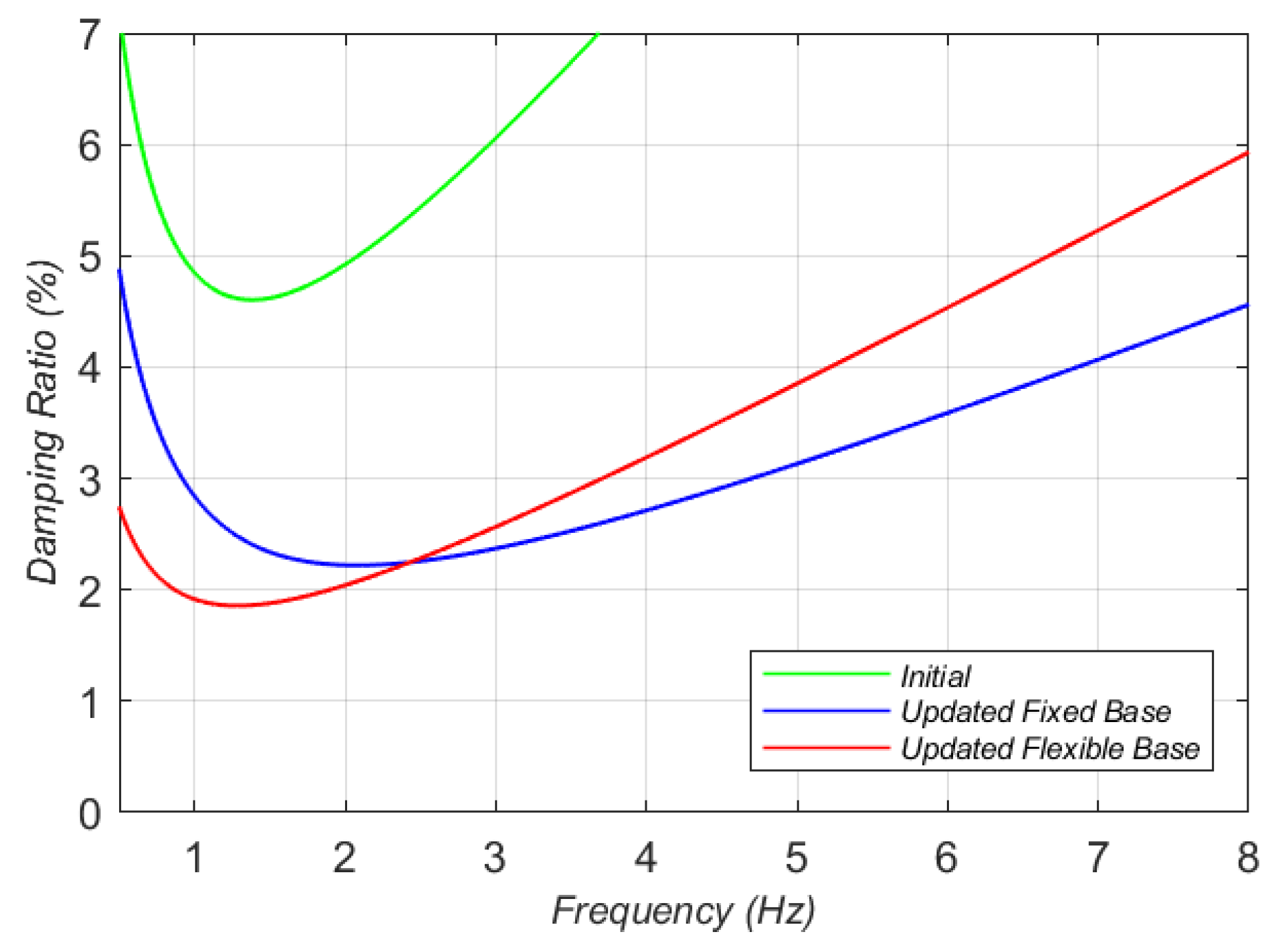
7.4. Rayleigh Damping

Figure 15 compares the Rayleigh damping ratio as a function of frequency between the initial, updated fixed-base, and updated flexible-base FE models. Table 6 shows that the estimated mass-proportional Rayleigh damping coefficient for the flexible-base structure is relatively small, which results in a nearly stiffness-proportional linear Rayleigh damping curve for the updated flexible-base model. This is a well-known effect of SSI on effective modal damping [48].

7.5. Possible Sources of Estimation Uncertainty

The estimated model parameters include uncertainties, which are quantified relatively using the estimated coefficient of variations (COVs). Aside from parameter identifiability issues, which are discussed earlier in the paper, modeling errors are most likely the most important source of estimation uncertainties. Modeling errors result from the inherent imperfections, approximations, and idealizations in the mathematical FE model. As a result, the selected class of FE models does not contain the real-world structure, and the estimated parameters characterize the closest possible model, in the model class, to the real structure [49]. Geometric approximations, material nonlinearities (even during low-amplitude earthquake excitations), effects of nonstructural components and systems, and modeling of damping energy dissipation mechanisms are some examples of imperfections in the numerical FE model. Model parameterization (i.e., selecting the estimation parameters in the model) is another source of modeling error. Modeling errors lead to biased estimation results. This means that by changing the earthquake event, the estimation result may vary, preferably slightly. Addressing the effects of modeling error requires repeating this study using more refined FE models and/or different earthquake data, which is beyond the scope of the present paper and can be the subject of future studies.

8. Conclusions

In this study, we developed a finite element (FE) model updating framework using a sequential Bayesian estimation approach to identify the soil and structural model parameters as well as the input motions from recorded seismic response of the Millikan Library building during the 2002 Yorba Linda earthquake. The newly developed Bayesian FE model updating procedure was used in a two-step system identification approach. In the first step, a fixed-base structural model was identified using partially unknown inputs. The structural model parameters included the effective stiffness of columns and shear walls (grouped along the height of the structure), the Rayleigh damping parameters, and the distributed floor mass. In the second step, the parameters characterizing the soil–structure model and the time histories of the Foundation Input Motions (FIMs) were estimated. The soil–structure model parameters included the soil subgrade and viscosity moduli at different foundation regions and the Rayleigh damping parameters. For each step, an identifiability analysis based on an information theoretic approach was performed to study the dependencies between model parameters and select the most identifiable parameter sets to be estimated. In Section 7 of the paper, the estimated model parameters were compared with the state-of-practice recommendations and other previous studies on the Millikan Library, and the differences were highlighted.
Minor differences were observed between the measured and FE-predicted response time histories obtained from the updated FE models. Considering the various sources of modeling error in this identification problem, the agreement between the updated FE model responses and the measurements was remarkable. Future studies are suggested to extend this process with more refined FE models (e.g., including material nonlinearities) and different earthquake data to further quantify the effects of modeling error. Applying this process to nonlinear SSI models using the recorded structural responses to strong ground motions may introduce additional complications due to the damage in nonstructural components, the nonlinear kinematic interaction between the structural and nonstructural systems, and the nonlinearities in the soil response. As a result, the identification of the nonlinear structural model parameters and the Raleigh damping model parameters is expected to include uncertainties and estimation biases. Furthermore, the identified soil–foundation subsystem model parameters, i.e., the impedance function, are expected to deviate more considerably from the state-of-practice recommendations. Despite these difficulties, undertaking such a research effort is crucial for developing a better understanding of the nonlinear interaction between the non-structure, structure, and soil subsystems. By utilizing the presented model inversion framework for different civil structures and earthquake records, key structural model parameters can be estimated from real-world seismic data. These are valuable information that can guide—along with theoretical results—the selection of engineering analysis and design parameters to improve state-of-the-art seismic analysis and design procedures.

Author Contributions

Conceptualization, H.E., F.G. and E.T.; methodology, H.E. and F.G.; software, H.E. and F.G.; val-idation, H.E. and A.T.; formal analysis, H.E., A.T., F.G. and E.T.; investigation, H.E., A.T. and F.G.; data curation, H.E. and A.T.; writing—original draft preparation, H.E. and A.T.; writing—review and editing, F.G. and E.T.; visualization, H.E. and A.T.; project administration, H.E. and D.A.; funding acquisition, H.E., D.A. and E.T. All authors have read and agreed to the published version of the manuscript.

Funding

This study was supported by the California Geological Survey through contracts no. 1016-987 and 1019-15, and the U.S. Geological Survey through grant no. G20AP00115-01. The supports are gratefully acknowledged. Any opinions, findings, conclusions, or recommendations expressed in this study are those of the authors and do not necessarily reflect the views of the sponsoring agencies.

Data Availability Statement

All data, models, or codes that support the findings of this study are available from the corresponding author upon reasonable request.

Conflicts of Interest

The authors declare no conflict of interest.

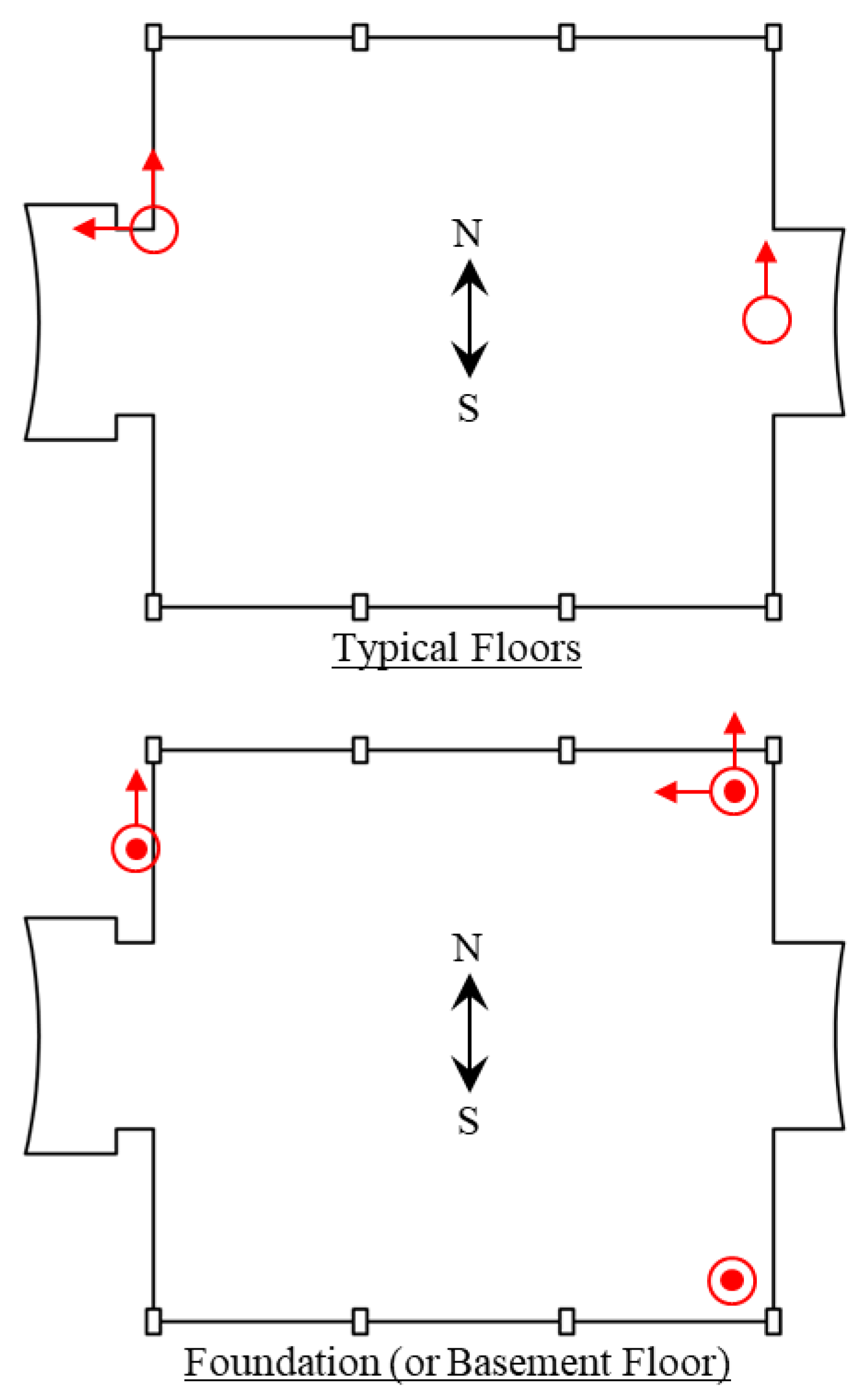
Appendix A. Instrumentation Plan for the Millikan Library

Table A1. Sensors’ locations and measurement directions.
Channel #Sensor LocationMeasurement
Direction
1Basement, North East CornerN
2Basement, North East CornerUp
3Basement, North East CornerE
4Basement, North West CornerN
5Basement, North West CornerUp
6Basement, South East CornerUp
71st Floor, EastN
81st Floor, WestE
91st Floor, WestN
102nd Floor, WestE
112nd Floor, WestN
123rd Floor, EastN
133rd Floor, WestE
143rd Floor, WestN
154th Floor, EastN
164th Floor, WestE
174th Floor, WestN
185th Floor, EastN
195th Floor, WestE
205th Floor, WestN
216th Floor, EastN
226th Floor, WestE
236th Floor, WestN
247th Floor, EastN
257th Floor, WestE
267th Floor, WestN
278th Floor, WestE
288th Floor, WestN
299th Floor, EastN
309th Floor, WestE
319th Floor, WestN
32Roof, EastN
33Roof, WestE
Figure A1. Floor plans showing the different sensors’ locations and measurement directions.
Buildings 13 00028 g0a1

References

  1. ASCE/SEI 7-10; Minimum Design Loads for Buildings and Other Structures. American Society of Civil Engineers: Reston, VA, USA, 2010.
  2. PEER. Guidelines for Performance-Based Seismic Design of Tall Buildings; Pacific Earthquake Engineering Research Center as part of the Tall Buildings Initiative, University of California: Berkeley, CA, USA, 2010. [Google Scholar]
  3. Stewart, J.; Crouse, C.; Hutchinson, T.; Lizundia, B.; Naeim, F.; Ostadan, F. Soil-Structure Interaction for Building Structures; Grant/Contract Reports (NISTGCR); National Institute of Standards and Technology (NIST): Gaithersburg, MD, USA, 2012.
  4. Roesset, J.M. A review of soil-structure interaction. In Soil-Structure Interaction: The Status of Current Analysis Methods and Research, Rep. No. NUREG/CR-1780 and UCRL; Nuclear Regulatory Commission: Washington, DC, USA, 1980. [Google Scholar]
  5. Tileylioglu, S.; Stewart, J.P.; Nigbor, R.L. Dynamic Stiffness and Damping of a Shallow Foundation from Forced Vibration of a Field Test Structure. J. Geotech. Geoenviron. Eng. 2011, 137, 344–353. [Google Scholar] [CrossRef] [Green Version]
  6. Jennings, P.C.; Kuroiwa, J.H. Vibration and soil-structure interaction tests of a nine-story reinforced concrete building. Bull. Seism. Soc. Am. 1968, 58, 891–916. [Google Scholar] [CrossRef]
  7. Wolf, J.P.; Deeks, A.J. Foundation Vibration Analysis: A strength of Materials Approach; Elsevier: Amsterdam, The Netherlands, 2004. [Google Scholar]
  8. Stewart, J.P.; Seed, R.B.; Fenves, G.L. Empirical Evaluation of Inertial Soil-Structure Interaction Effects; Pacific Earthquake Engineering Research Center: Berkeley, CA, USA, 1998. [Google Scholar]
  9. Pais, A.L.; Kausel, E. On rigid foundations subjected to seismic waves. Earthq. Eng. Struct. Dyn. 1989, 18, 475–489. [Google Scholar] [CrossRef]
  10. Luco, J.E.; Westmann, R.A. Dynamic Response of a Rigid Footing Bonded to an Elastic Half Space. J. Appl. Mech. 1972, 39, 527–534. [Google Scholar] [CrossRef]
  11. Ebrahimian, H.; Astroza, R.; Conte, J.P.; Papadimitriou, C. Bayesian optimal estimation for output-only nonlinear system and damage identification of civil structures. Struct. Control. Health Monit. 2018, 25, e2128. [Google Scholar] [CrossRef]
  12. Ebrahimian, H.; Astroza, R.; Conte, J.P. Extended Kalman filter for material parameter estimation in nonlinear structural finite element models using direct differentiation method. Earthq. Eng. Struct. Dyn. 2015, 44, 1495–1522. [Google Scholar] [CrossRef]
  13. Astroza, R.; Ebrahimian, H.; Conte, J.P. Material Parameter Identification in Distributed Plasticity FE Models of Frame-Type Structures Using Nonlinear Stochastic Filtering. J. Eng. Mech. 2015, 141. [Google Scholar] [CrossRef]
  14. Ebrahimian, H.; Astroza, R.; Conte, J.P.; de Callafon, R.A. Nonlinear finite element model updating for damage identification of civil structures using batch Bayesian estimation. Mech. Syst. Signal Process. 2016, 84, 194–222. [Google Scholar] [CrossRef]
  15. Beck, J.L.; Katafygiotis, L.S. Updating models and their uncertainties. I: Bayesian statistical framework. J. Eng. Mech. ASCE 1998, 124, 455–462. [Google Scholar] [CrossRef]
  16. Beck, J.L. Bayesian system identification based on probability logic. Struct. Control. Health Monit. 2010, 17, 825–847. [Google Scholar] [CrossRef]
  17. Simon, D. Optimal State Estimation: Kalman, H infinity, and Nonlinear Approaches; John Wiley & Sons: Hoboken, NJ, USA, 2006. [Google Scholar]
  18. Astroza, R.; Ebrahimian, H.; Conte, J.P. Batch and Recursive Bayesian Estimation Methods for Nonlinear Structural System Identification; Springer: Berlin/Heidelberg, Germany, 2017; pp. 341–364. [Google Scholar] [CrossRef]
  19. Conte, J.P.; Vijalapura, P.K.; Meghella, M. Consistent Finite-Element Response Sensitivity Analysis. J. Eng. Mech. 2003, 129, 1380–1393. [Google Scholar] [CrossRef] [Green Version]
  20. McKenna, F. OpenSees: A Framework for Earthquake Engineering Simulation. Comput. Sci. Eng. 2011, 13, 58–66. [Google Scholar] [CrossRef]
  21. MathWorks. MATLAB 2022a, MathWorks: Natick, MA, USA, 2022.
  22. Simon, D.; Simon, D.L. Constrained Kalman filtering via density function truncation for turbofan engine health estimation. Int. J. Syst. Sci. 2010, 41, 159–171. [Google Scholar] [CrossRef]
  23. Ebrahimian, H.; Kohler, M.; Massari, A.; Asimaki, D. Parametric estimation of dispersive viscoelastic layered media with application to structural health monitoring. Soil Dyn. Earthq. Eng. 2018, 105, 204–223. [Google Scholar] [CrossRef]
  24. Kuroiwa, J.H. Vibration Test of a Multistory Building; Caltech: Pasadena, CA, USA, 1967. [Google Scholar]
  25. Crouse, C.B.; Jennings, P.C. Soil-structure interaction during the San Fernando earthquake. Bull. Seism. Soc. Am. 1975, 65, 13–36. [Google Scholar] [CrossRef]
  26. Luco, J.E.; Trifunac, M.D.; Wong, H.L. On the apparent change in dynamic behavior of a nine-story reinforced concrete building. Bull. Seism. Soc. Am. 1987, 77, 1961–1983. [Google Scholar] [CrossRef]
  27. Bradford, S.C.; Clinton, J.F.; Favela, J.; Heaton, T.H. Results of Millikan Library Forced Vibration Testing; Caltech: Pasadena, CA, USA, 2004. [Google Scholar]
  28. Ghahari, S.F.; Abazarsa, F.; Avci, O.; Çelebi, M.; Taciroglu, E. Blind identification of the Millikan Library from earthquake data considering soil-structure interaction. Struct. Control Health Monit. 2015, 23, 684–706. [Google Scholar] [CrossRef]
  29. Taciroglu, E.; Ghahari, S.; Abazarsa, F. Efficient model updating of a multi-story frame and its foundation stiffness from earthquake records using a timoshenko beam model. Soil Dyn. Earthq. Eng. 2017, 92, 25–35. [Google Scholar] [CrossRef]
  30. Shirzad-Ghaleroudkhani, N.; Mahsuli, M.; Ghahari, S.F.; Taciroglu, E. Bayesian identification of soil-foundation stiffness of building structures. Struct. Control Health Monit. 2017, 25, e2090. [Google Scholar] [CrossRef]
  31. CESMID. Center for Engineering Strong Motion Data. Available online: https://www.strongmotioncenter.org/ (accessed on 10 October 2022).
  32. Computers and Structures. SAP2000. Available online: https://www.csiamerica.com/products/sap2000 (accessed on 10 October 2022).
  33. Ebrahimian, H.; Asimaki, D.; Kusanovic, D.; Ghahari, S.F. Untangling the Dynamics of Soil-Structure Interaction Using Nonlinear Finite Element Model Updating. In Proceedings of the SMIP17 Conference on Utilization of Strong-Motion Data, Berkeley, CA, USA, 19 October 2017. [Google Scholar]
  34. Ebrahimian, H.; Astroza, R.; Conte, J.P.; Bitmead, R.R. Information-Theoretic Approach for Identifiability Assessment of Nonlinear Structural Finite-Element Models. J. Eng. Mech. 2019, 145. [Google Scholar] [CrossRef]
  35. Brun, R.; Reichert, P.; Künsch, H.R. Practical identifiability analysis of large environmental simulation models. Water Resour. Res. 2001, 37, 1015–1030. [Google Scholar] [CrossRef] [Green Version]
  36. Yu, E.; Taciroglu, E.; Wallace, J.W. Parameter identification of framed structures using an improved finite element model-updating method—Part I: Formulation and verification. Earthq. Eng. Struct. Dyn. 2006, 36, 619–639. [Google Scholar] [CrossRef]
  37. Foutch, D.A.; Jennings, P.C. A study of the apparent change in the foundation response of a nine-story reinforced concrete building. Bull. Seism. Soc. Am. 1978, 68, 219–229. [Google Scholar] [CrossRef]
  38. Todorovska, M.I. Soil-Structure System Identification of Millikan Library North-South Response during Four Earthquakes (1970-2002): What Caused the Observed Wandering of the System Frequencies? Bull. Seism. Soc. Am. 2009, 99, 626–635. [Google Scholar] [CrossRef] [Green Version]
  39. ACI 318-14; Building Code Requirements for Structural Concrete and Commentary. American Concrete Institute: Farmington Hills, MI, USA, 2014.
  40. Pais, A.; Kausel, E. Approximate formulas for dynamic stiffnesses of rigid foundations. Soil Dyn. Earthq. Eng. 1988, 7, 213–227. [Google Scholar] [CrossRef]
  41. Wong, H.; Trifunac, M.; Luco, J. A comparison of soil-structure interaction calculations with results of full-scale forced vibration tests. Soil Dyn. Earthq. Eng. 1988, 7, 22–31. [Google Scholar] [CrossRef]
  42. Veletsos, A.S.; Meek, J.W. Dynamic behaviour of building-foundation systems. Earthq. Eng. Struct. Dyn. 1974, 3, 121–138. [Google Scholar] [CrossRef]
  43. He, X.; Moaveni, B.; Conte, J.P.; Elgamal, A.; Masri, S.F. System Identification of Alfred Zampa Memorial Bridge Using Dynamic Field Test Data. J. Struct. Eng. 2009, 135, 54–66. [Google Scholar] [CrossRef]
  44. Luco, J.E.; Trifunac, M.D.; Wong, H.L. Isolation of soil-structure interaction effects by full-scale forced vibration tests. Earthq. Eng. Struct. Dyn. 1988, 16, 1–21. [Google Scholar] [CrossRef]
  45. Cheng, M.H.; Heaton, T.H. Simulating Building Motions Using Ratios of the Building’s Natural Frequencies and a Timoshenko Beam Model. Earthq. Spectra 2015, 31, 403–420. [Google Scholar] [CrossRef] [Green Version]
  46. Balendra, T.; Tat, C.W.; Lee, S.-L. Modal damping for torsionally coupled buildings on elastic foundation. Earthq. Eng. Struct. Dyn. 1982, 10, 735–756. [Google Scholar] [CrossRef]
  47. Freddi, F.; Galasso, C.; Cremen, G.; Dall’Asta, A.; Di Sarno, L.; Giaralis, A.; Gutiérrez-Urzúa, F.; Málaga-Chuquitaype, C.; Mitoulis, S.A.; Petrone, C.; et al. Innovations in earthquake risk reduction for resilience: Recent advances and challenges. Int. J. Disaster Risk Reduct. 2021, 60, 102267. [Google Scholar] [CrossRef]
  48. Cruz, C.; Miranda, E. Evaluation of soil-structure interaction effects on the damping ratios of buildings subjected to earthquakes. Soil Dyn. Earthq. Eng. 2017, 100, 183–195. [Google Scholar] [CrossRef]
  49. Ghahari, S.F.; Sargsyan, K.; Çelebi, M.; Taciroglu, E. Quantifying modeling uncertainty in simplified beam models for building response prediction. Struct. Control Health Monit. 2022, 29, e3078. [Google Scholar] [CrossRef]
Figure 1. Millikan Library building.
Buildings 13 00028 g001
Figure 2. Developed FE model of the Millikan Library structure.
Buildings 13 00028 g002
Figure 3. Relative entropy gain of the fifteen model parameters (see Table 2 for parameter IDs).
Buildings 13 00028 g003
Figure 4. Relative mutual entropy gain between the parameter pairs (see Table 2 for parameter IDs).
Buildings 13 00028 g004
Figure 5. Relative root mean square error (RRMSE) between the measured and the FE predicted structural responses using the initial and final FE models.
Buildings 13 00028 g005
Figure 6. Comparison of the measured and estimated acceleration response time histories at Channels #4 and #5. The right-hand-side plots magnify the response time history between 1 and 7 s. Each figure’s title shows the sensor location and recording direction, e.g., “Basement, North West Corner-Z” means acceleration response time history in the Z-direction, recorded by the sensor located on the north-west corner of the basement.
Buildings 13 00028 g006
Figure 7. Comparison of the measured structural responses with the structural responses predicted using the initial and final-updated FE models for both Case 1 and Case 2. The right-hand-side plots magnify the response time history between 1 and 7 s. Each figure’s title shows the sensor location and recording direction, e.g., “9th floor, East-N” means acceleration response time history in the NS direction, recorded by the sensor located on the east side of the 9th floor.
Buildings 13 00028 g007
Figure 8. Structural configuration of the Millikan Library basement showing the structural walls and two-level foundation details, including the central pad (at EL.−6 m from the ground surface), and the two north and south foundation beams (at EL.−5 m from the ground surface).
Buildings 13 00028 g008
Figure 9. (a) Six unknown subgrade modulus parameters, and (b) six unknown viscosity modulus parameters defined for different foundation regions. The figures show the foundation plan of the Millikan library, including the central pads, and the two foundation beams (dimensions are in meters).
Buildings 13 00028 g009
Figure 10. Relative entropy gain of the fifteen model parameters (see Table 5 for parameter IDs).
Buildings 13 00028 g010
Figure 11. Relative mutual entropy gains between the parameter pairs (see Table 5 for parameter IDs).
Buildings 13 00028 g011
Figure 12. (a) Estimated foundation input motion (FIM) time histories and (b) their standard deviation (SD) values.
Buildings 13 00028 g012
Figure 13. Comparison of the measured structural responses with the structural responses predicted using the final estimates of the soil-structure model parameters and FIMs. The left-hand-side plots compare the responses in frequency domain, the middle plots compare the time histories, and the right-hand-side plots magnify the response time history between 1 and 7 s.
Buildings 13 00028 g013
Figure 14. Relative root mean square error (RRMSE) of the FE predicted structural responses using the final estimates of the soil–structure model parameters.
Buildings 13 00028 g014
Figure 15. The Rayleigh damping ratio as a function of frequency in the initial, updated fixed-base, and updated flexible-base FE models.
Buildings 13 00028 g015
Table 1. Sequential FE model updating algorithm for joint estimation of model parameters and input motion time histories.
1.
Determine the start and end points of the estimation windows—i.e., t 1 m , t 2 m ,
where m = 1, 2, …, N and N is the number of estimation windows.
2.
Set the initial mean vector and covariance matrix of the model parameter vector ( θ ^ 0 , P ^ θ 0 ) and input ground motion time history vector across the first estimation window ( u ¨ ^ 0 , t 1 1 : t 2 1 g , P ^ u ¨ 0 g ). The initial mean values of the ground motion time history are usually set as zero, i.e., u ¨ ^ 0 , t 1 1 : t 2 1 g = 0 .
3.
Use the inverse of the initial values of the model parameters as the scaling factors, i.e., a n = 1 θ 0 , n . Set up ψ ^ 0 , 0 + = [ A θ ^ 0 u ¨ ^ 0 , t 1 1 : t 2 1 g ] T and P ^ ψ , 0 , 0 + = [ A P ^ θ 0 A T 0 0 P ^ u ¨ 0 g ] .
4.
For the mth estimation window:
4.1.
Setup the initial mean vector and covariance matrix of the unknown parameters (i.e., ψ ^ m , 0 + and P ^ ψ , m , 0 + ) based on the posterior mean vector and covariance matrix obtained from the last estimation window (i.e., ψ ^ m 1 + and P ^ ψ , m 1 + ) (refer to [11] for details).
4.2.
Define the process noise covariance matrix Q and the simulation error covariance matrix R. Set up R ˜ .
4.3.
Iterate (j = 1, 2, …):
4.3.1.
Set ψ ^ m , j = ψ ^ m , j 1 + , P ^ ψ , m , j = P ^ ψ , m , j 1 + + Q .
4.3.2.
Obtain the FE responses using ψ ^ m , j , i.e., y ^ t 1 m : t 2 m = h t 1 m : t 2 m ( ψ ^ m , j , u ¨ ^ 1 : t 1 m 1 g ) . Obtain the FE response sensitivities using a finite difference method. Set up the sensitivity matrix with respect to the scaled model parameters, C s .
4.3.3.
Compute the Kalman gain matrix: K = ( P ^ ψ , m , j ( C s ) T ) ( C s P ^ ψ , m , j ( C s ) T + R ˜ ) 1 .
4.3.4.
Find the corrected estimates of the mean vector and covariance matrix of the extended parameter vector:
ψ ^ m , j + = ψ ^ m , j + K ( y t 1 m : t 2 m h t 1 m : t 2 m ( ψ ^ m , j , u ¨ ^ 1 : t 1 m 1 g ) ) , ⋯ P ^ ψ , m , j + = ( I K C s ) P ^ ψ , m , j ( I K C s ) T + K R ˜ K T .
4.3.5.
Correct for constraints.
4.3.6.
Update the model parameter scaling factors using Equation (8). Update ψ ^ m , j + and P ^ ψ , m , j + based on the new model parameter scale factors.
4.3.7.
Check for convergence: if | ψ ^ m , j + ψ ^ m , j 1 + | < 0.01 × | ψ ^ m , j 1 + |   or   j > 15 , then move to the next estimation window (m = m + 1, go to step 4); otherwise, iterate again at the current estimation window (j = j + 1, go to step 4.3).
Table 2. Fifteen model parameters used for prior model identifiability assessment.
Parameter IDDescriptionValue
1Elastic modulus of brace elements representing precast claddings20 GPa
2Effective elastic modulus of beam and slab concrete at 1st floor5.8 GPa
3Effective elastic modulus of beam and slab concrete at 2nd floor5.8 GPa
4Effective elastic modulus of beam and slab concrete at 3rd floors5.8 GPa
5Effective elastic modulus of beam and slab concrete at 4th, 5th, and 6th floors5.8 GPa
6Effective elastic modulus of beam and slab concrete at 7th, 8th, 9th, and roof floors5.8 GPa
7Effective elastic modulus of column and wall concrete at basement17.3 GPa
8Effective elastic modulus of column and wall concrete at 1st story17.3 GPa
9Effective elastic modulus of column and wall concrete at 2nd story17.3 GPa
10Effective elastic modulus of column and wall concrete at 3rd, 4th, and 5th stories17.3 GPa
11Effective elastic modulus of column and wall concrete at 6th, 7th, 8th, 9th, and roof stories17.3 GPa
12Mass-proportional Rayleigh damping coefficient0.4
13Stiffness-proportional Rayleigh damping coefficient5.3 × 10−3
14Distributed floor mass on 1st to 9th floors250 kg/m2
15Distributed floor mass on roof300 kg/m2
Table 3. Final selected model parameters for Step 1 system identification.
Parameter IDDescriptionValue
1Elastic modulus of brace elements representing precast claddings (EClad)20 GPa
2Effective elastic modulus of column and wall concrete at basement and 1st story (EW&C1)17.3 GPa
3Effective elastic modulus of column and wall concrete at 2nd story to roof (EW&C2)17.3 GPa
4Mass-proportional Rayleigh damping coefficient (α)0.4
5Stiffness-proportional Rayleigh damping coefficient (β)5.3 × 10⁻³
6Distributed floor mass on 1st to roof floors (m) 250 kg/m2
Table 4. Initial and final estimates of the model parameters, along with their final estimated coefficient of variation (COV). Parameters are defined in Table 3.
ParameterECladEW&C1EW&C2αβm
Initial Estimate20 GPa17.3 GPa17.3 GPa0.405.3 × 10−3250 kg/m2
Case 1—Final Estimate (COV)0.25 GPa
(9.87%)
16.2 GPa
(0.41%)
29.7 GPa
(0.68%)
0.24
(2.64%)
2.6 × 10⁻³
(1.4%)
2.8 kg/m2
(8.97%)
Case 2—Final Estimate (COV)6.17 GPa
(2.87%)
19.6 GPa
(0.66%)
26.1 GPa
(0.84%)
0.29
(2.61%)
1.7 × 10⁻³
(2%)
161 kg/m2
(2.44%)
Table 5. Fifteen model parameters used for prior model identifiability assessment.
Parameter ID12345678
Parameterkxky1ky2kz1kz2kz3cxcy1
Value65
MN/m3
100
MN/m3
150
MN/m3
20
MN/m3
22.5
MN/m3
37.5
MN/m3
700
kN.s/m3
700
kN.s/m3
Parameter ID9101112131415
Parametercy2cz1cz2cz3αβEFound
Value700
kN.s/m3
1000 kN.s/m31000 kN.s/m31000 kN.s/m30.291.7 × 10−37.5
GPa
Table 6. Initial and final estimates of the soil–structure model parameters along with their final estimated coefficient of variation (COV).
Parameterkxkykz1kz2kz3
Initial Estimate200 MN/m3200 MN/m3225 MN/m3225 MN/m3225 MN/m3
Final Estimate
(COV)
47.9 MN/m3 (2.7%)418.2 MN/m3 (4.9%)386.8 MN/m3 (0.9%)614.4 MN/m3 (3.4%)310.5 MN/m3 (3.4%)
Parametercxcyczαβ
Initial Estimate700 kN.s/m3700 kN.s/m31000 kN.s/m30.291.7 × 10−3
Final Estimate (COV)313.7 kN.s/m3 (13.1%)1187 kN.s/m3 (10.7%)4 kN.s/m3 (906.5%)0.15
(3.1%)
2.3 × 10⁻³
(2%)
Table 7. Comparison of the normalized estimated lumped stiffness and viscosity of the soil–foundation subsystem with the recommended values in [3]. The translational components are normalized by GL and the rotational components by GL3, where G = 268 MPa and 2L = 27.4 m.
Foundation Vibration ModeTrans.-EWTrans.-NSTrans.-UpRock.-EWRock.-NSTorsion
Estimated Stiffness5.850.6559.082.151.382.14
NIST-based Stiffness5.145.276.086.163.987.08
Estimated Viscosity0.040.140.00050.000020.000010.007
NIST-based Viscosity0.130.130.230.0050.0040.038
Table 8. Comparison of the normalized lumped stiffness of soil–foundation subsystem between different studies. The translational components are normalized by GL and the rotational components by GL3, where G = 268 MPa and 2L = 27.4 m.
StudyFoundation Vibration Mode
Trans.-EWTrans.-NSRock.-EWRock.-NSTorsional
[6]31.18.7207.2145.99.9–10.5
[44]6.94.610.05.4
[41]7.26.710.25.9
[26]5.55.27.45.611.1
[45]2.72.71.81.8
[28]6.22.53.90.98
Current Study5.1450.652.151.382.14
Table 9. Comparison of the flexible-based and fixed-base modal periods of the updated FE models.
Structural Vibration Mode1st Trans.-EW1st Trans.-NS1st Torsional2nd Trans.-EW2nd Trans.-NS
Flexible-base Period (s)0.950.60.420.220.16
Fixed-base Period (s)0.880.50.370.20.16
Period Elongation1.081.21.141.11.0
Disclaimer/Publisher’s Note: The statements, opinions and data contained in all publications are solely those of the individual author(s) and contributor(s) and not of MDPI and/or the editor(s). MDPI and/or the editor(s) disclaim responsibility for any injury to people or property resulting from any ideas, methods, instructions or products referred to in the content.

