Metamodel-Based Hyperparameter Optimization of Optimization Algorithms in Building Energy Optimization

Abstract

Building energy optimization (BEO) is a promising technique to achieve energy efficient designs. The efficacy of optimization algorithms is imperative for the BEO technique and is significantly dependent on the algorithm hyperparameters. Currently, studies focusing on algorithm hyperparameters are scarce, and common agreement on how to set their values, especially for BEO problems, is still lacking. This study proposes a metamodel-based methodology for hyperparameter optimization of optimization algorithms applied in BEO. The aim is to maximize the algorithmic efficacy and avoid the failure of the BEO technique because of improper algorithm hyperparameter settings. The method consists of three consecutive steps: constructing the specific BEO problem, developing an ANN-trained metamodel of the problem, and optimizing algorithm hyperparameters with nondominated sorting genetic algorithm II (NSGA-II). To verify the validity, 15 benchmark BEO problems with different properties, i.e., five building models and three design variable categories, were constructed for numerical experiments. For each problem, the hyperparameters of four commonly used algorithms, i.e., the genetic algorithm (GA), the particle swarm optimization (PSO) algorithm, simulated annealing (SA), and the multi-objective genetic algorithm (MOGA), were optimized. Results demonstrated that the MOGA benefited the most from hyperparameter optimization in terms of the quality of the obtained optimum, while PSO benefited the most in terms of the computing time.

1. Introduction

1.1. Background

The growth in global energy consumption has raised concerns about primary energy shortages and serious environmental impacts, such as global warming, ozone layer depletion, and climate change. According to the International Energy Agency, buildings consume nearly 36% of the world’s energy and are responsible for 39% of global greenhouse gas emissions [1]. Thus, building designs that emphasize energy efficiency are crucial to reducing carbon emissions, achieving energy savings, and adapting to climate change.

Several energy-efficient building technologies have been proposed to improve building energy efficiency, among which the building energy optimization (BEO) technique has emerged as a promising method to achieve high-performance design, with particular emphasis on building energy. It has been revealed that it can reduce building energy use by up to 30 percent compared to a benchmark design [2]. The general procedure of the BEO technique is illustrated in Figure 1. As shown, it relies on optimization algorithms to create new designs according to preset design objectives and simulation results. This technique has been widely applied in optimizing building systems (such as lighting and HVAC), building envelopes (such as form, construction, and double-skin facades) and renewable energy generation (such as solar and ground energy) [3].

As illustrated in Figure 1, the optimization algorithm plays a vital role in the BEO workflow. The algorithm drives the whole technical process, automatically adjusts the design variables to generate new designs, and regularly finds an optimal design that meets the predefined objective. Therefore, the efficacy of an algorithm significantly affects the efficiency of the BEO technique. Currently, there are a variety of optimization tools can be integrated into the BEO technique [4], including GenOpt, modeFRONTIER, ModelCetner, Matlab, jEPlusþEA, MOBO, ENEROPT, GENE_ARCH, and Grasshopper plugins, such as Galapagos, Goat, Silvereye, Opossum, Optimus, RBFMopt, and Dodo. Among them, MATLAB is one of the most often used [5] and was adopted in this study. These optimization tools are often embedded with various optimization algorithms which generally fall into three categories: direct search, intelligent optimization, and hybrid. Our previous review found that [5] intelligent algorithms are the most popular in BEO, followed by direct search algorithms. Among intelligent algorithms, the genetic algorithm (GA) and its modified versions are dominant, followed by the particle swarm optimization (PSO) algorithm. Although many algorithms are currently used, not all algorithms work well for any given BEO problem. Figure 2 illustrates the general working mechanism of optimization algorithms. Starting from one or several initial solutions, a certain strategy is applied to guide the next search for new solutions, the search is stopped when the termination conditions are met, and finally, the optimal solution examined in the run is output. Therefore, the selection of the initial solutions, the strategy of searching for new solutions, and the hyperparameters of the algorithm that implement the searching strategy determine the search path, and thus determine the algorithm’s global search ability and the overall running time.

Considering the crucial role of hyperparameters in algorithm efficacy and BEO efficiency, they should be accurately set to maximize the optimization ability of the algorithm so as to quickly and exactly find the global optimum. However, existing works targeting algorithm hyperparameters in BEO are rare. Effective methods for setting algorithm hyperparameters are still lacking. Due to barriers related to expertise, the current BEO research simply uses the common general hyperparameter settings (HPSs) indiscriminately without considering their validity and reliability. However, obtaining a general-purpose, universal HPS is impossible. The algorithm hyperparameters should be accurately tuned based on the specific BEO problem to be solved.

A challenge faced by tuning the HPS of an algorithm applied in BEO is the computationally expense of building energy evaluation. Generally, three types of models can be used to perform building energy evaluation: simplified analytical models, detailed simulation models and metamodels (or surrogate models). Simplified analytical models aim to establish mathematical functions between design variables and building energy by describing physical mechanisms. This kind of work can be found in [6]. Although mathematical formulas can be quickly calculated, describing a BEO problem mathematically is not easy. In most cases, the BEO problem is too complicated to allow its physical mechanism to be captured, especially with high dimension of design variables or complex building models. Therefore, simplified analytical models are only applicable to simple problems. Detailed simulation models are most frequently used in BEO. Much related work can be found in [7,8,9,10], where various programs were used, including EnergyPlus, TRNSYS, IDA-ICE, DOE2, etc. A major challenge faced in detailed models is the high computational cost, where one simulation can take minutes, hours, or even days. Consequently, design optimization, sensitivity analysis, and design space exploration become impracticable as they often require hundreds or thousands of simulation evaluations. One method of alleviating this burden is by developing metamodels that mimic the behavior of the detailed simulation models using a data-driven, bottom-up approach [11]. Metamodeling, also known as black-box modeling, behavioral modeling, or surrogate modeling, is trained on the basis of modeling the simulator’s response to a limited number of samples. It has been receiving increasing attention in a wide range of applications in building design; for example, sensitivity analysis [12], uncertainty analysis [13], and optimization [14]. Several methods have been successfully used to train metamodels in BEO, such as ANNs, Bayesian networks, support vector machines (SVMs), etc. Among them, ANNs have been proven to have high accuracy for learning, strong capacity for nonlinear mapping, and good robustness, and have been actively used in building-related studies; for example, building energy [15,16], thermal load [17], and daylighting prediction [18]. To fit an ANN model into different problems, its hyperparameters also must be tuned and optimized. It is crucial to select an appropriate technique to detect optimal hyperparameters of ANNs. The commonly used techniques include grid search, random search, Bayesian optimization, gradient-based optimization, and metaheuristic algorithms, such as GA and PSO.

1.2. Literature Review

1.2.1. The Efficacy of Optimization Algorithms in BEO

In view of the crucial role of algorithms in BEO technique, their efficacy has attracted the attention of building energy related research. Related works include Prada et al. [19], which compared the efficacy of three algorithms used for evaluating the optimal refurbishment of three reference buildings. The authors focused on two efficacy criteria of the algorithms, namely, the percentage of actual Pareto solutions and the number of cost function assessments, where the actual Pareto front was determined through a brute-force approach. Waibel et al. [20] investigated the performance behavior of a widely selected single-objective black-box optimization algorithms, including deterministic, randomized, and model-based algorithms. They also studied the effect of hyperparameters on the efficacy of the algorithms. The efficacy criteria of interest for these algorithms included convergence times, stability, and robustness. Chegari et al. [21] applied the BEO technique with integrated multilayer feedforward neural networks (MFNNs) to optimize the indoor thermal comfort and energy consumption of residential buildings. They compared the computation time required by the three most commonly used metaheuristic algorithms, i.e., the multi-objective genetic algorithm (MOGA), the nondominated sorting genetic algorithm II (NSGA-II), and the multi-objective particle swarm optimization (MOPSO). The results indicated that MOPSO performed the best. Si et al. developed sets of efficacy criteria for single-objective and multi-objective algorithms [22,23]. They also investigated the ineffectiveness of algorithms and the causal factors that may lead to ineffectiveness, including the selection of the initial designs and HPSs [24].

1.2.2. Methods of Setting Algorithm Hyperparameters in BEO

At present, four methods of setting algorithm hyperparameters can be found in BEO-related works. One is to simply use the default HPSs of the algorithms embedded in mature optimization tools described in Section 1.1. Related studies include that of Yu et al. [7], which applied NSGA-II to optimize thermal comfort and energy efficiency in a building design. NSGA-II was realized in MATLAB and run with the default HPS in the tool. Hamdy et al. [25] compared seven commonly used multi-objective evolutionary algorithms in solving a nearly zero-energy building design problem. Due to lacking scientific information on the algorithm hyperparameters for building energy problems, they employed the default HPSs in MATLAB. In these studies, the algorithms’ default HPSs in the optimization tools were assumed to be generally applicable for most problems. However, this assumption is unfair. In fact, most optimization tools (e.g., modeFRONTIER and MATLAB) were originally developed to solve problems encountered in non-architectural fields, such as mathematics and computer science. Whether the default HPSs for non-architectural problems apply to BEO problems is still an open question. One fact is that the requirements for the optimization capabilities of algorithms differ with the problems faced by different research fields. For example, the objective calculations of mathematics problems are generally fast when using mathematical software such as MATLAB, usually less than one second. Thus, compared with the computation cost, the quality of the final optimum obtained by algorithms is more significant in mathematics. However, the objective calculations of building models are usually time-consuming, ranging from minutes to hours when using detailed building simulation models. Considering the limited computing time, the available number of objective calculations for BEO problems is usually 100–1000 orders of magnitude less than that for mathematics problems. Thus, both the computation time and the quality of the final optimum are essential for BEO technique. In this case, the default HPSs that are valid for a mathematics problem may not have the same effect for a BEO problem.

The second common method is to manually evaluate algorithms’ efficacy with a limited number of HPSs and then choose the one that makes the algorithm perform best. Related studies include that of Wright and Alajmi [8], who investigated the robustness of a GA in finding solutions to an unconstrained building optimization problem. Experiments were performed for twelve different HPSs of GA, with nine trial optimizations completed for each HPS. Yang et al. [26] performed a sensitivity analysis to investigate the effects of two algorithm hyperparameters, namely, the number of generations and population size, on the optimal trade-off solution and the robustness of NSGA-II. Chen et al. [27] applied NSGA-II to optimize passively designed buildings. Different HPSs of NSGA-II were examined to improve the computational efficiency without jeopardizing the optimization productivity. In this area, due to the limitations of manual tuning and comparison, the number of hyperparameter combinations is usually inadequate, which leaves a large portion of possible combinations uninvestigated. In this case, the result is only the best in the compared group, not the real best in the whole feasible region.

The third widely used method in BEO for setting algorithm hyperparameters is to learn from the HPSs used in other similar studies or from the expertise of researchers. Related studies include that of Futrell et al. [28], which presented a methodology to optimize daylighting performance of a complex building design using dynamic climate-based lighting simulations. The authors compared four optimization algorithms and used HPSs that have performed well in other similar publications. Delgarm et al. [9] coupled a mono- and multi-objective PSO algorithm with EnergyPlus to search for a set of Pareto solutions to improve building energy performance. The hyperparameters of PSO were set up based on the authors’ expertise. Ascione et al. [29] proposed a new methodology for the evaluation of cost-optimality through the multi-objective optimization. The HPS of the GA were determined based on the expertise of the authors and some previous studies. Such methods in this sector still have limitations. On the one hand, most HPSs used in the referenced studies were initially identified through manual comparison studies or by using the default HPSs in optimization tools. Their reliability still needs to be further verified; blindly learning from other works will lead to unreliable optimization results. On the other hand, due to the diversity of building models, building design variables, and optimization objectives, the BEO problems to be solved are diverse. It is quite difficult for designers to find similar research to directly borrow their HPSs.

The fourth method involves using self-adaptive strategies to generate algorithmic hyperparameters, which allows the algorithm itself to be adapted to the characteristics of the problem. Related works include that of Cubukcuoglu et al. [30], which proposed a new optimization tool named Optimus for grasshopper algorithmic modeling in Rhinoceros CAD software. It implemented a self-adaptive differential evolution algorithm with an ensemble of mutation strategies (jEDE) which performed better than most other optimization tools in the tests of standard and CEC 2005 benchmark problems. Ramallo-González and Coley [31] used a self-adaptive differential evolution algorithm (jDE) to cope with changes in the objective landscape for low-energy building design optimization. Ekici et al. [32] adopted a multi-objective jDE in the conceptual phase to solve a form-finding problem in high-rise building design. Results indicated that jDE outperformed NSGA-II with a much more desirable Pareto front. Although self-adaptive strategies have shown their strengths in most works, in most cases, they only focused on limited algorithm hyperparameters; for example, the mutation rate of the differential evolution algorithm without considering other algorithm hyperparameters simultaneously and the interactions between them.

1.2.3. Summary of the Literature Review

The efficacy of optimization algorithms has raised concerns in the BEO research field. Although algorithm hyperparameters have a significant impact on algorithm efficacy, studies focusing on this topic are insufficient, and there still exist some unsolved problems: (1) the four common methods for setting algorithm hyperparameters fail to fully evaluate the possible combinations and interactions; (2) due to the variety of BEO problems, algorithm parameters should be set up based on the properties involved in the problem, such as multidimensionality, building types, optimization objectives, etc.; however, studies focusing on problems’ properties are scare.

1.3. Research Outline

This paper aims to fill these knowledge gaps and address the abovementioned issues by intelligently optimizing the HPSs of algorithms applied in BEO. The outline of this paper is as follows:

• A metamodel-based methodology for hyperparameter optimization of algorithms applied in BEO is introduced;
• A total of 15 benchmark BEO problems with different properties are constructed for numerical experiments;
• The HPSs of four commonly used algorithms are optimized.

The research presented in this paper is timely and valuable for a number of reasons. On the theoretical side, the proposed method can deepen our understanding of algorithm hyperparameters, the efficacy of algorithms and the properties of BEO problems in general. On the application side, the results obtained from this study can help engineers, architects, and consultants properly set algorithm hyperparameters so as to effectively apply the BEO technique and use various energy-saving measures.

The rest of this paper is organized as follows: Section 2 illustrates the methodology; Section 3 presents a step-by-step detailed numerical experiment; Section 4 offers the results and discussion; Section 5 summarizes the paper and discusses the challenges of this study and the prospects for future research.

2. Methodology

The workflow of the proposed methodology is summarized in Figure 3. As shown, it mainly includes three steps: constructing the specific BEO problem, developing the metamodel of the problem, and hyperparameter optimization of the algorithm applied in BEO. Detailed explanations of each step are given below.

2.1. Step 1: Constructing the Specific BEO Problem

Generally, the mathematical form of a BEO problem can be as follows:

$$\underset{xϵX}{argmin}F\left(X\right)={\left[f_1\left(X\right),f_2\left(X\right),\dots ,f_k\left(X\right)\right]}^T$$

(1)

$$Subject to: g_i\left(X\right)=0, i=1,2,\dots ,p$$

$$h_j\left(X\right)\ge 0,j=1,2,\dots ,q$$

where X is a vector of n design variables, k ≥ 1 is the number of optimization objectives, F(X) ∈ R_k is the vector of objective functions in which f_i(X) is the computation function of the ith objective, and g_i(X) and h_j(X) are equality and inequality constraints, respectively. If p and q equal 0, this is an unconstrained optimization problem. If k equals 1, the problem is a single-objective optimization problem. By convention, Equation (1) defines a minimization problem. A maximization problem can be solved by converting the objective function into a minimization problem.

According to the expression shown in Equation (1), design variables, objective functions, and constraints are the key elements of a BEO problem, and they are often computationally expensive to simulate, multimodal, non-smooth, non-differentiable, etc. [33] These properties contribute to the complexity of BEO problems and may seriously exacerbate the difficulty of algorithm optimization. For example, the high dimensions of input and output variables make problem modeling and optimization exponentially difficult. As the number of design variables increases, the search space expands exponentially, which dramatically increases the difficulties for algorithms in searching the entire design space. In these cases, it is more important to accurately set the algorithm parameters to help the algorithm effectively overcome specific property obstacles and achieve efficient optimization. Hence, the first step of the developed method is to construct the clear BEO problem to be solved, including the building model, design variables, constraints, and optimization objectives, and then optimizing the HPSs of the algorithm to overcome the property barriers involved in the specific problem.

2.2. Step 2: Developing the Metamodel of the BEO Problem

The hyperparameter optimization of an algorithm needs to investigate the efficacy of the algorithm when adopting different HPSs. Each adjustment of the HPS requires the BEO workflow illustrated in Figure 1 to run once. In this case, the total computing time T can be roughly calculated by Equation (2):

$$T={\sum }_{k=1}^m{n}_k\times \Delta t$$

(2)

where m is the total number of HPS adjustments, n_k is the number of building designs generated by the BEO process with the kth HPS tuning, and Δt is the computing time consumed in evaluating the energy objective of a design.

It is clear that Δt is crucial to the total computing time T. As introduced in Section 1.1, among the three evaluation methods of building energy, including simplified analytical models, detailed simulation models and metamodels, metamodels demonstrate great advantages in terms of accuracy and time cost. In this study, an ANN is chosen as the metamodeling technique. The general procedure for ANN-trained meta-modeling is as follows:

• Sampling input variables and using detailed building simulation tools to calculate the corresponding energy consumption of each sample to form a database for metamodel training;
• Based on the sample database, training the metamodel by ANN;
• Hyperparameter optimization of ANN and verifying the accuracy of the metamodel.

2.3. Step 3: Hyperparameter Optimization of Algorithms

Hyperparameter optimization of an algorithm needs to constantly tune the HPSs to determine the one that makes the algorithm perform best. If relying on manual tuning, the process will be time consuming and may be unable to fully evaluate the feasible domain of the hyperparameters. In addition, when the feasible domain of the hyperparameters are continuous, there are theoretically infinite possible values, making it impossible to manually traverse all the possibilities. Therefore, to overcome the trial-and-error limitations of manual tuning, this study employs NSGA-II to automatically tune the HPSs and finally output the optimum.

Figure 4 illustrates the flowchart of Step 3, which essentially involves two optimization loops. The inner loop is driven by a test algorithm that requires hyperparameter optimization. It solves the specific BEO problem modeled by the ANN. The outer optimization loop is driven by NSGA-II, which automatically tunes the HPSs of the test algorithm. For each adjustment, the inner loop is run accordingly, and the efficacy of the test algorithm is assessed. The outer loop ends when reaching the termination condition of NSGA-II, and the optimal HPS of the test algorithm over the whole computing run is output. The optimization objectives of the outer loop are the efficacy criteria of optimization algorithms proposed in our previous works [22,23], which aim to quantitatively describe the different performance aspects of algorithms applied in BEO. Specifically, the performance criteria for single-objective test algorithms include (1) the quality of the optimal design obtained, (2) the computing time, and (3) the diversity of all designs searched in an optimization run. The performance criteria for multi-objective test algorithms include (1) the number of Pareto solutions, (2) the quality of the Pareto solutions, (3) the diversity of the Pareto solutions, and (4) the computing time. In practice, users are recommended to select the criteria they care most about. Furthermore, the reasons for choosing NSGA-II as the optimizer of the outer loop are manifold. NSGA-II is one of the most commonly used algorithms in engineering optimization. Its robustness to HPSs has been verified as good in some previous works [34,35]. Moreover, appropriate HPSs for NSGA-II have been suggested in some previous works and have been successfully applied in some implementations. Andersson et al. [36] suggested the HPS for NSGA-II as a crossover rate of 0.9, a mutation rate of 0.008, and a population size of 100.

3. Numerical Experiments

3.1. Step 1: Constructing 15 Benchmark BEO Problems with Different Properties

3.1.1. Benchmark Buildings

To investigate the applicability and reliability of the proposed methodology, a set of BEO problems with different properties was constructed based on the DOE benchmark commercial buildings [37]. Five new-construction building types, namely, small office, medium office, large office, primary school, and large hotel, were modified. Specifically, overhangs were added to the original DOE models to investigate their impact on building energy and thermal comfort. All these buildings were located in Baltimore, Maryland, in the 4A climate zone according to the US standard. Figure 5 shows the architectural schematic views of the five building models and

Table 1. Summary of the characteristics of the benchmark models.

Building Type	Form							HVAC
	Building Shape	Aspect Ratio	Number of Floors	Floor to Ceiling Height (m)	Floor to Floor Height (m)	Total Floor Area (m2)	Number of Conditioned Zones	System Type	Heating Type	Cooling Type	Fan Control
Small Office	Rectangle	1.5	1	3.1	-	511	5	PSZ-AC 1	Gas furnace	Unitary DX 2	Constant volume
Medium Office	Rectangle	1.5	3	2.7	4.0	4982	15	MZ-VAV 3	Gas furnace and electric reheat	PACU 4	Variable
Large Office	Rectangle	1.5	12 plus basement	2.74	3.96	46,320	61	MZ-VAV	Gas boiler	2 water cooled chillers	Variable
Primary School	“E” Shape	-	1	4	-	6871	25	CAV 5, PSZ-AC (gym, kitchen, & cafeteria)	Gas boiler, gas furnace (gym, kitchen, & cafeteria)	PACU	Constant
Large Hotel	Rectangle	3.8 1st floor, 5.1 other floors	6 plus basement	3.96 1st floor, 3.05 other floors	3.96 1st floor, 3.05 other floors	11,345	195	FCU 6 in rooms, CV 7 ventilation, MZVAV 8 in common areas	Gas boiler	2 air cooled chillers	Variable

¹ packaged single zone air conditioner (PSZ-AC); ² direct expansion system (DX); ³ multi-zone variable air volume (MZ-VAV); ⁴ packaged air conditioning unit (PACU); ⁵ constant air volume (CAV); ⁶ fan coil unit (FCU); ⁷ constant volume (CV); ⁸ multizone variable air volume (MZVAV).

summarizes their characteristics.

3.1.2. Design Variables

In the case studies, a maximum of 30 design variables related to building energy consumption and thermal comfort were selected.

Table 2. Specifications of the optimization variables.

Categories	Description of Design Variables	Symbol	Unit	Properties	Range	Step Size
Building orientation	Building long axis azimuth	x1	°	Discrete	0–180	1
Thermostats set-points	Cooling set-point temperature	x2	°C	Discrete	22–29	1
	Heating set-point temperature	x3	°C	Discrete	15–22	1
Roof insulation properties	Roof insulation conductivity	x4	W/m·K	Continuous	0.03–0.06	0.001
	Roof insulation thickness	x5	m	Continuous	0.01–0.15	0.001
Opaque wall insulation conductivity	South wall insulation conductivity	x6	W/m·K	Continuous	0.03–0.06	0.001
	East wall insulation conductivity	x7	W/m·K	Continuous	0.03–0.06	0.001
	North wall insulation conductivity	x8	W/m·K	Continuous	0.03–0.06	0.001
	West wall insulation conductivity	x9	W/m·K	Continuous	0.03–0.06	0.001
Exterior wall insulation thickness	South wall insulation thickness	x10	m	Continuous	0.01–0.15	0.001
	East wall insulation thickness	x11	m	Continuous	0.01–0.15	0.001
	North wall insulation thickness	x12	m	Continuous	0.01–0.15	0.001
	West wall insulation thickness	x13	m	Continuous	0.01–0.15	0.001
Window size	South window upper position	x14	m	Continuous	1–2.7	0.01
	East window upper position	x15	m	Continuous	1–2.7	0.01
	North window upper position	x16	m	Continuous	1–2.7	0.01
	West window upper position	x17	m	Continuous	1–2.7	0.01
Window U-value	South window U-value	x18	W/m2·K	Continuous	1–7	0.01
	East window U-value	x19	W/m2·K	Continuous	1–7	0.01
	North window U-value	x20	W/m2·K	Continuous	1–7	0.01
	West window U-value	x21	W/m2·K	Continuous	1–7	0.01
Window SHGC	South window SHGC	x22	-	Continuous	0.1–0.9	0.01
	East window SHGC	x23	-	Continuous	0.1–0.9	0.01
	North window SHGC	x24	-	Continuous	0.1–0.9	0.01
	West window SHGC	x25	-	Continuous	0.1–0.9	0.01
Window external shading	South window overhang depth	x26	m	Continuous	0.02–2	0.01
	East window overhang depth	x27	m	Continuous	0.02–2	0.01
	North window overhang depth	x28	m	Continuous	0.02–2	0.01
	West window overhang depth	x29	m	Continuous	0.02–2	0.01
	Shading transmittance	x30	-	Continuous	0–1	0.01

lists their symbols, units, and ranges of variation, as well as step sizes for discrete variables. As shown, one variable describes building orientation, which is continuous and has a great impact on the solar heat gain through the facade. Two variables are related to the cooling and heating set-point temperatures, which significantly impact the energy consumed by the mechanical system and the indoor thermal comfort. Optimizing the heat transfer through opaque walls and roofs is of great significance in designing high performance buildings. In this study, the conductivity and thickness of the insulation layers in the roofs and opaque walls were described and optimized by ten continuous design variables. Windows are usually the least insulated part of the envelope and determine the amount of indoor daylight and the view of the outside. Therefore, in the present case studies, the window sizes and the thermal properties of the windows (e.g., the solar heat gain coefficient (SHGC) and U-Factor), which have a critical impact on the indoor thermal comfort and energy, were considered. To easily define the size of a window, its lower position was fixed at 0.9 m, and only its upper position was changed. In addition, the windows on the same facade have equal areas. As shown in Figure 5, overhangs exist along the upper sides of the windows. The depths of the overhangs and their transmittances were optimized; these control the light and heat that enter the building through the windows. Moreover, the depths of the overhangs in the same façade were kept the same.

As introduced in Section 2.2, the multidimensional property of a BEO problem determines the difficulty of optimization algorithms in searching the entire design space. In this study, three types of optimization problems with different dimensions, i.e., 10, 20, and 30 design variables, respectively, were constructed for each building model shown in Figure 5. Specifically, for problems with n design variables, the first n design variables listed in Table 2 were selected. In summary, a total of 15 BEO problems are constructed in this study.

3.1.3. Optimization Objectives

The optimization objectives in BEO research include energy, cost, comfort, etc., among which energy is considered most often. In the numerical experiments, we constructed two types of problems, i.e., single-objective and multi-objective problems. In particular, minimizing the annual energy consumption (AEC) was defined for single-objective optimizations, while two conflicting objectives, minimizing the AEC vs. maximizing the indoor thermal comfort (ITC), were considered simultaneously in multi-objective optimizations. The AEC is calculated as the total amount of energy consumed throughout the year. The common methods of evaluating indoor thermal comfort include the predicted percentage of dissatisfied (PPD) (0–100%) and the predicted mean vote (PMV). They are assessed based on the Fanger thermal comfort model [38], which is widely used in air-conditioned buildings [11]. In this study, the annual averaged PPD (AAPPD) over all zones during occupied times for one year was used and is calculated as follows:

$$AAPPD=\frac{1}{n}{\sum }_{i=1}^n{\sum }_{t=1}^{12}PP{D}_{i,t}$$

(3)

where n is the total number of conditioned zones and PPD_i,t is the average PPD in zone i in the tth month of a year. In this case, maximizing the thermal comfort is converted into minimizing the AAPPD.

3.2. Step 2: Developing Metamodels of the Benchmark BEO Problems

3.2.1. Creating ANN Modeling Datasets

An important preliminary step in ANN modeling is to create training data sets. In this study, the Latin hypercube sampling (LHS) method embedded in the modeFRONTIER software was applied to create the design samples for each benchmark problem.

EnergyPlus was integrated with modeFRONTIER to automatically simulate the AEC and AAPPD of the samples. McKay [39] and Asadi et al. [40] found that it was sufficient to correctly characterize the search space when the number of cases sampled using LHS exceeded twice the number of design parameters. Therefore, the number of samples gathered for each BEO problem is equal to 50 times the number of inputs times the number of outputs. For example, for a bio-objective optimization problem with 30 design variables, 3000 design samples were generated. The time consumed for objective simulation of design samples is summarized in

Table 3. ANN training and validation results.

Building Type	Number of Design Variables	Number of Hidden Neurons	Sampling Size	Sampling Time (h)	ANN Training Results
					Training		Validation		Testing
					MSE	R	MSE	R	MSE	R
Small office	10	10	1000	6.6	0.019	0.9999	0.025	0.9999	0.027	0.9999
	20	10	2000	13.3	0.032	0.9999	0.075	0.9999	0.086	0.9999
	30	20	3000	20	0.037	0.9999	0.093	0.9999	0.113	0.9999
Medium office	10	10	1000	9.7	0.019	0.9999	0.03	0.9999	0.021	0.9999
	20	20	2000	19.4	0.048	0.9999	0.103	0.9999	0.1	0.9999
	30	26	3000	29.1	0.073	0.9999	0.231	0.9999	0.255	0.9999
Large office	10	10	1000	11.9	0.046	0.9999	0.062	0.9999	0.056	0.9999
	20	25	2000	23.9	0.21	0.9999	0.518	0.9999	0.59	0.9999
	30	30	3000	35.8	0.986	0.9999	1.923	0.9998	1.813	0.9998
Primary school	10	15	1000	16.4	0.083	0.9999	0.133	0.9999	0.115	0.9999
	20	25	2000	32.8	0.038	0.9999	0.184	0.9999	0.156	0.9999
	30	25	3000	49.2	0.142	0.9999	0.382	0.9999	0.478	0.9999
Large hotel	10	10	1000	21.1	0.084	0.9999	0.098	0.9999	0.021	0.9999
	20	20	2000	42.2	0.048	0.9999	0.154	0.9999	0.164	0.9999
	30	30	3000	63.3	0.097	0.9999	0.199	0.9999	0.225	0.9999

. Finally, the input (sample designs) and output (corresponding AEC and AAPPD) data were imported into the neural network toolbox of MATLAB to train and validate ANN models. The normalized sample distribution of benchmark problems with 30 design variables is illustrated in Figure 6. As shown, the value range of each variable is uniformly covered.

3.2.2. ANN Training and Validation

Before ANN modeling for a benchmark problem, as suggested by Shahin et al. [41], the sampling dataset was randomly divided into a training set, a validation set, and a test set based on the ratio of 70%, 15%, and 15%, respectively. As shown in Figure 7, the ANN employed in this study is a three-layer feedforward network containing a hidden layer. The neurons in the input layer receive data from the design variables, while the neurons in the output layer provide the prediction outcomes of the design objectives. Between the two layers, the number of neurons in the hidden layer is detected by means of a trial-and-error method according to the average relative error of ANN predictions (Table 3). The Levenberg–Marquardt backpropagation algorithm [42,43] was applied to train the network. The transfer functions included a sigmoidal function for the hidden layer and a linear function for the output layer. Similar network configurations have been employed in previous notable studies concerning BEO with very sound results [44,45]. When the mean square error (MSE) of the validation samples was stable, the training process stopped automatically. Specifically, MSE was the average squared difference between the original EnergyPlus simulations and the ANN predictions. Lower MSE values are better, and zero means there is no error. Furthermore, the coefficient of correlation (R) between the predictions and original simulations were calculated to further assess the ANN model. Since the test set did not participate in training, it was employed to independently assess the network performance during and after training by considering the distribution of the MSE and R. Table 3 reported the ANN testing results for each metamodel. As illustrated in Table 3, the R values were all very close to 1 for each benchmark BEO problem, and the MSEs were quite small, demonstrating great agreement between the simulations and the predictions.

3.3. Step 3: Hyperparameter Optimization of the Test Algorithms

3.3.1. Test Algorithms and Hyperparameters

This study investigates three commonly used single-objective optimization algorithms, i.e., the GA, the PSO, and the simulated annealing (SA) algorithm, and one multi-objective optimization algorithm, namely, MOGA. All algorithms were implemented in the global optimization toolbox of MATLAB. Detailed descriptions of each algorithm and their working strategies are provided in Ref. [46].

Table 4. Hyperparameters of the test optimization algorithms, their ranges, and default values in MATLAB.

Algorithms	Hyperparameters	Description	Minimum	Maximum	Default
GA	PopulationSize	Number of individuals in each generation.	5	200	200
	EliteRate	Positive integer specifying the proportion of individuals from the current generation surviving to the next. EliteCount = cell(EliteRate×PopulationSize)	0.01	0.99	0.05
	CrossoverFraction	The fraction of the population at the next generation created by the crossover function, excluding elite children. Mutation produces the remaining individuals in the next generation.	0	1	0.8
	MaxStallGenerations	The algorithm stops if the average relative change in the best fitness function value over MaxStallGenerations generations is equal to or less than FunctionTolerance.	2	200	50
PSO	SwarmSize	Number of particles in the swarm.	5	200	min(100, 10 × nvars), where nvars is the number of variables
	InertiaRange_LowerLimit	The lower bound of the adaptive inertia.	0	1	0.1
	InertiaRange_UpperLimit	The upper bound of the adaptive inertia.	1	2	1.1
	MinNeighborsFraction	Minimum adaptive neighborhood size.	0	1	0.25
	SelfAdjustmentWeight	The weight of the best position of each particle when adjusting velocity.	0	2	1.49
	SocialAdjustmentWeight	The weight of the best position of neighborhood when adjusting velocity.	0	2	1.49
	MaxStallIterations	Number of iterations over which the relative change in best objective function value is less than options.FunctionTolerance.	2	200	20
SA	ReannealInterval	The number of points to accept before reannealing.	1	200	100
	InitialTemperature	The temperature at the beginning of the run.	1	200	100
	MaxStallIterations	Number of iterations over which average change in objective function value at current point is less than options.FunctionTolerance	2	4000	500 × number of variables
MOGA	PopulationSize	Number of individuals in each generation.	5	200	200
	CrossoverFraction	The fraction of the population at the next generation created by the crossover function, excluding elite children. Mutation produces the remaining individuals in the next generation.	0	1	0.8
	MaxStallGenerations	Number of stall generations over which the average relative change in the best fitness function value is less than or equal to FunctionTolerance.	2	200	100

lists the hyperparameters of the algorithms and their descriptions along with the default values in MATLAB for comparative studies.

3.3.2. Performance Evaluation Criteria of the Test Algorithms

In our previous works, a set of criteria was proposed to evaluate the overall performance of an optimization algorithm [22,23]. As each criterion reflects a different performance aspect of an algorithm, there is no common agreement that one criterion is more important than the others. As suggested in Ref. [23], the importance of each criterion is mainly dependent on the needs of the users according to their specific requirements. In engineering practice, the most common demand for optimization algorithms is to find a desired design within a restricted runtime. Therefore, this study mainly focuses on two conflicting efficacy aspects, i.e., the quality of the optimal design obtained by the algorithm and the computing time. Generally, if an algorithm is pressured to converge quickly to an optimum, it will explore less of the searchable design space and may converge to a mediocre optimum. Similarly, if the algorithm strives to diversify the areas it explores in search of better designs, it may consume more computing time in evaluating the explored designs, especially when using the simulation models with high computation cost. In this sense, an algorithm that converges quickly and locates the desired optimum is preferred.

For a single-objective algorithm, which locates a unique optimum in an optimization run, the method of calculating the quality of the located optimal design is to directly evaluate the objective value of the design. When the multi-objective algorithm finally locates a set of nondominated solutions in an optimization run, one possible method is to first distinguish the ideal Pareto design on the Pareto front by the weighted sum model (WSM) method coupled with the min-max normalization method (Figure 8), and then evaluate the quality of the selected ideal design by assessing its objective values. As a result, the ideal design satisfies (in the minimization case) Equation (4):

$$R_{WSM-score}^{*}=\underset{i}{\min }{\sum }_{j=1}^m{\omega }_j\frac{f_i^j-f_{min}^j}{f_{max}^j-f_{min}^j},\hspace{1em}\mathrm{for} i=1,2,\dots ,n,$$

(4)

where R*_WSM-score is the WSM score of the ideal design, f_i^j is the objective value of the ith Pareto-optimal design in the jth optimization objective, f_min^j and f_max^j are, respectively, the minimum and maximum values of the jth optimization objective that the optimization run reaches, ω_j ≥ 0 is the importance of the jth objective, n is the total number of Pareto-optimal designs, and m is the number of optimization objectives. The method of evaluating the computing time of an optimization run is to calculate the total number of building simulations when it terminates, which reflects the number of designs found by the algorithm during the run. It is noted that all the test algorithms terminated when one of the following two conditions was met. One is that over MaxStallGenerations or MaxStallIterations generations, the average relative change of the best objective value reaches FunctionTolerance, which was set as 10⁻³. The other is the total number of objective function evaluations should not exceed 3000, which corresponds to the maximum number of samples generated to build metamodels in Section 3.2.1.

3.3.3. Method for Identifying the Specific Optimal HPS from the Pareto Front of NSGA-II

Since the outer loop shown in Figure 4 is a multi-objective optimization run driven by NSGA-II, it locates multiple nondominated solutions on the Pareto front when NSGA-II terminates, and each solution corresponds to an HPS of the test algorithm. In theory, each HPS on the Pareto front is desirable, but it is still necessary to select the ideal one for application and evaluation. Thus, the WSM method is used to make multi-objective decisions for these nondominated solutions. To eliminate the unit differences between the two efficacy evaluation criteria of test algorithms, i.e., the quality of the obtained optimum and the computing time, the value of each criterion is first normalized using the max-min normalization method as in Equation (5). Then, a weight is assigned to each criterion based on its importance. Finally, the sum of the products of the normalized values of each evaluation criterion and its weight is calculated as in Equation (6). The ideal HPS identified from the Pareto front of NSGA-II is the one with the smallest R value.

$$P_i^j=\frac{p_i^j-p_{min}^j}{p_{max}^j-p_{min}^j}$$

(5)

$$R^{*}=\underset{i\in \left\{1,\dots ,n\right\}}{\min }{\sum }_{j=1}^m{w}_j{P}_i^j$$

(6)

where n is the total number of Pareto-optimal solutions searched by NSGA-II, m is the number of algorithm efficacy evaluation criteria, which is 2 in this study, and w_j is the weight of the jth evaluation criterion. This study assumes that the quality of the searched optimum and the computation time are equally important for the test algorithms, so their weights are both set to 1.

4. Results and Discussion

4.1. Numerical Experiment Results

For different benchmark problems, the hyperparameter optimization convergence graphs of the four test algorithms are illustrated in

Table A1. The hyperparameter optimization convergence graphs of the four test algorithms.

	Small office_10 Variables	Small office_20 Variables	Small office_30 Variables
GA
PSO
SA
MOGA
	Medium office_10 variables	Medium office_20 variables	Medium office_30 variables
GA
PSO
SA
MOGA
	Large office_10 variables	Large office_20 variables	Large office_30 variables
GA
PSO
SA
MOGA
	Primary school_10 variables	Primary school_20 variables	Primary school_30 variables
GA
PSO
SA
MOGA
	Large hotel_10 variables	Large hotel_20 variables	Large hotel_30 variables
GA
PSO
SA
MOGA

The black dots are non-dominant solutions, and the gray dots are dominant solutions.

of Appendix A. The finally identified ideal HPS of the test algorithms are listed in

Table 5. Optimal HPSs for the GA.

Building Type	Number of Design Variables	Ideal HPS				Optimal Design with the Optimal HPS		Optimal Design with the Default HPS
		Population Size	Elite Rate	Crossover Fraction	MaxStall Generations	AEC	NS	AEC	NS
Small office	10	43	0.208	0.545	61	112.078	2838	112.784	3000
	20	15	0.183	0.736	197	100.999	2985	103.239	3000
	30	23	0.011	0.705	93	98.941	2415	103.755	3000
Medium office	10	32	0.09	0657	64	129.339	2144	130.303	3000
	20	12	0.12	0.595	109	111.188	1572	112.733	3000
	30	23	0.078	0.636	85	111.053	2783	118.060	3000
Large office	10	30	0.053	0.674	70	134.869	2160	134.917	3000
	20	25	0.09	0.66	91	125.019	2325	125.744	3000
	30	24	0.129	0.545	97	120.357	2424	124.123	3000
Primary school	10	38	0.209	0.63	64	148.317	2546	148.975	3000
	20	13	0.038	0.673	121	129.829	2288	134.101	3000
	30	64	0.027	0.662	21	128.399	2752	139.556	3000
Large hotel	10	31	0.11	0.562	77	376.323	2449	376.711	3000
	20	11	0.069	0.691	162	371.637	1804	372.689	3000
	30	37	0.17	0.464	69	354.797	2849	370.098	3000

,

Table 6. Optimal HPSs for the PSO.

Building Type	Number of Design Variables	Optimal HPS							Optimal Design with the Optimal HPS		Optimal Design with the Default HPS
		Swarm Size	Inertia Range_Lower Limit	Inertia Range_Upper Limit	Min Neighbors Fraction	Self Ajustment Weight	Social Adjustment Weight	MaxStall Iterations	AEC	NS	AEC	NS
Small office	10	6	0.32	1.66	0.39	0.4	0.87	2	111.774	48	111.774	2600
	20	11	0.54	1.35	0.55	1.71	1.14	51	98.902	1155	99.242	3000
	30	19	0.6	1.88	0.5	0.39	0.94	35	93.935	2983	96.412	3000
Medium office	10	5	0.38	1.66	0.34	0.44	0.96	12	128.461	115	128.461	2600
	20	7	0.59	1.49	0.38	0.27	1.23	18	107.375	322	107.375	3000
	30	40	0.49	1.36	0.18	1.41	1.84	20	107.285	3000	111.771	3000
Large office	10	6	0.5	1.66	0.07	0.12	0.84	34	134.751	384	134.758	3000
	20	13	0.27	1.71	0.33	1.53	1	65	124.315	2197	125.005	3000
	30	13	0.53	1.84	0.5	0.42	0.84	36	118.499	2119	122.805	3000
Primary school	10	6	0.48	1.67	0.55	1.08	0.86	34	148.026	288	148.027	2700
	20	17	0.55	1.98	0.55	1.63	0.7	35	123.162	2397	126.351	3000
	30	20	0.54	1.52	0.01	0.92	0.96	60	125.131	2940	131.892	3000
Large hotel	10	5	0.51	1.38	0.41	0.41	0.86	5	376.117	35	376.117	2300
	20	10	0.46	1.99	0.53	1.02	0.81	130	371.178	1940	371.436	3000
	30	18	0.54	1.99	0.53	0.11	0.86	50	345.59	2232	350.763	3000

,

Table 7. Optimal HPSs for the SA.

Building Type	Number of Design Variables	Optimal HPS			Optimal Design with the Optimal HPS		Optimal Design with the Default HPS
		Reanneal Interval	Initial Temperature	MaxStall Iterations	AEC	NS	AEC	NS
Small office	10	73	153	798	112.437	1181	113.032	3000
	20	195	172	2050	103.655	2407	105.460	3000
	30	46	185	1005	101.926	1341	106.408	3000
Medium office	10	73	146	1142	128.548	1958	130.689	3000
	20	92	183	1814	114.657	2899	126.053	3000
	30	98	178	569	120.539	1150	128.539	3000
Large office	10	106	150	514	134.997	1904	135.371	3000
	20	105	141	1038	126.399	1795	129.199	3000
	30	121	134	1026	123.8	1413	127.724	3000
Primary school	10	97	154	514	148.658	802	149.523	3000
	20	30	73	516	134.275	886	145.251	3000
	30	97	178	694	136.297	2986	143.401	3000
Large hotel	10	124	172	514	376.663	1120	383.958	3000
	20	117	164	520	372.553	1341	381.068	3000
	30	108	171	2058	360.193	2327	371.517	3000

and

Table 8. Optimal HPSs for the MOGA.

Building Type	Number of Design Variables	Optimal HPS			Optimal Design with the Ideal HPS			Optimal Design with the Default HPS
		Population Size	Crossover Fraction	MaxStall Generations	AEC	AAPPD	NS	AEC	AAPPD	NS
Small office	10	9	0.181	124	136.216	14.29	1144	137.114	14.460	3000
	20	13	0.416	178	123.319	12.974	2354	125.394	14.343	3000
	30	11	0.476	43	116.407	11.584	2278	121.165	14.401	3000
Medium office	10	9	0.392	197	145.916	12.382	1801	146.672	12.924	3000
	20	14	0.119	5	127.41	4.854	2773	134.193	8.643	3000
	30	17	0.359	149	106.728	5.652	2585	128.215	8.450	3000
Large office	10	59	0.272	38	138.832	11.657	2892	138.832	11.659	3000
	20	37	0.177	52	126.688	5.375	2443	131.168	8.356	3000
	30	6	0.459	16	126.814	6.719	2317	130.538	8.672	3000
Primary school	10	41	0.802	66	160.077	9.632	2830	160.687	9.886	3000
	20	27	0.103	91	141.412	6.997	2566	156.687	8.667	3000
	30	39	0.553	39	126.718	6.933	1912	151.296	8.613	3000
Large hotel	10	23	0.276	33	386.818	15.644	2301	387.896	16.562	3000
	20	14	0.71	135	382.304	14.014	2045	385.635	15.941	3000
	30	45	0.243	2	378.843	13.796	2971	384.560	14.435	3000

. For BEO problems with the same complexities as the 15 benchmark problems constructed in this study, Table 5, Table 6, Table 7 and Table 8 offer guidance for users in setting hyperparameters for the four test algorithms. In this case, users can use the detailed simulation models to calculate building performance without developing metamodels, as the results are trade-offs between the quality of the obtained optimum and the computing time.

4.2. Comparison with the Default HPSs in MATLAB

To validate the proposed methodology, this section compares the efficacy differences of the test algorithms on each evaluation criterion when they use the identified ideal HPSs and the default HPSs in MATLAB. As shown in

Table 9. Differences in the quality of the optimum and the number of simulations when the test algorithms use the optimal HPSs and the default ones.

Building Type	Number of Design Variables	GA		PSO		SA		MOGA
		AEC	NS	AEC	NS	AEC	NS	AEC	AAPPD	NS
Small office	10	−0.63%	−5.40%	0	−98.15%	−0.53%	−60.63%	−0.65%	−1.18%	−61.87%
	20	−2.17%	−0.50%	−0.34%	−61.50%	−1.71%	−19.77%	−1.65%	−9.54%	−21.53%
	30	−4.64%	−19.50%	−2.57%	−0.57%	−4.21%	−55.30%	−3.93%	−19.56%	−24.07%
Medium office	10	−0.74%	−28.53%	0	−95.58%	−1.64%	−34.73%	−0.52%	−4.19%	−39.97%
	20	−1.37%	−47.60%	0	−89.27%	−9.04%	−3.37%	−5.05%	−43.84%	−7.57%
	30	−5.94%	−7.23%	−4.01%	0	−6.22%	−61.67%	−16.76%	−33.11%	−13.83%
Large office	10	−0.04%	−28.00%	−0.01%	−87.20%	−0.28%	−36.53%	0%	−0.02%	−3.60%
	20	−0.58%	−22.50%	−0.55%	−26.77%	−2.17%	−40.17%	−3.42%	−35.67%	−18.57%
	30	−3.03%	−19.20%	−3.51%	−29.37%	−3.07%	−52.90%	−2.85%	−22.52%	−22.77%
Primary school	10	−0.44%	−15.13%	0	−89.33%	−0.58%	−73.27%	−0.38%	−2.57%	−5.67%
	20	−3.19%	−23.73%	−2.52%	−20.10%	−7.56%	−70.47%	−9.75%	−19.27%	−14.47%
	30	−7.99%	−8.27%	−5.13%	−2.00%	−4.95%	−0.47%	−16.24%	−19.51%	−36.27%
Large hotel	10	−0.10%	−18.37%	0	−98.48%	−1.90%	−62.67%	−0.28%	−5.54%	−23.30%
	20	−0.28%	−39.87%	−0.07%	−35.33%	−2.23%	−55.30%	−0.86%	−12.09%	−31.83%
	30	−4.13%	−5.03%	−1.47%	−25.60%	−3.05%	−22.43%	−1.49%	−4.43%	−0.97%

, the number of simulations was greatly reduced, with reduction rates ranging from 0.5% to 47.6% for GA, 0 to 98.48% for PSO, 0.47% to 73.27% for SA, and 0.97% to 61.87% for MOGA. The reduction in the number of simulations is significantly helpful for BEO problems, especially for time-consuming performance simulations when using detailed simulation models. As shown in Figure 9, for all the 15 benchmark problems, the NS reduction of PSO is generally large, indicating that the running time of PSO is more dependent on its hyperparameters, and the final optimum can be found faster by hyperparameter optimization of PSO. Moreover, among the other three algorithms, SA benefited more from hyperparameter optimization in terms of NS, with the general largest NS reduction.

Regarding the quality of the optimums obtained by the test algorithms when solving the 15 benchmark problems, compared with the default HPSs, the AEC variation range of the GA, PSO, SA, and the MOGA when using the optimal HPSs is −7.99–−0.04%, −5.13–0%, −9.04–−0.28%, and −16.76–0%, respectively. The AAPPD variation range of MOGA is −43.84–−0.02%. As illustrated in Figure 10, the MOGA generally benefited the most from hyperparameter optimization with the highest reductions of AEC and AAPPD. Among the three single-objective algorithms, hyperparameter optimization is shown most favorable to SA, followed by the GA. By contrast, PSO had the smallest improvement in the quality of the optimum, which demonstrated an insensitivity to hyperparameters; therefore, hyperparameter optimization is mainly beneficial to the running time of PSO.

4.3. Efficacy Comparison between the Test Algorithms

To compare the efficacy of the three single-objective test algorithms when they use the identified optimal HPSs, we first ranked them in terms of the two specific performance assessment criteria and illustrated the ranking results in

Table 10. Ranking results of the optimal design quality obtained by the three single-objective test algorithms when using the optimal HPSs.

Building Type	Number of Design Variables	Ranking
		GA	PSO	SA
Small office	10	2	1	3
	20	2	1	3
	30	2	1	3
Medium office	10	3	1	2
	20	2	1	3
	30	2	1	3
Large office	10	2	1	3
	20	2	1	3
	30	2	1	3
Primary school	10	2	1	3
	20	2	1	3
	30	2	1	3
Large hotel	10	2	1	3
	20	2	1	3
	30	2	1	3

and

Table 11. Ranking results of the number of simulations required by the three single-objective test algorithms when using the optimal HPSs.

Building Type	Number of Design Variables	Ranking
		GA	PSO	SA
Small office	10	3	1	2
	20	3	1	2
	30	2	3	1
Medium office	10	3	1	2
	20	2	1	3
	30	2	3	1
Large office	10	3	1	2
	20	3	2	1
	30	3	2	1
Primary school	10	3	1	2
	20	2	3	1
	30	1	2	3
Large hotel	10	3	1	2
	20	2	3	1
	30	3	1	2

. As shown in Table 10, for the same benchmark problem, PSO generally found a better design than the other two algorithms and always came out on top, while SA exhibited the worst performance behavior, always ranking third. In addition, according to Table 11, the GA performed the worst in terms of the number of simulations, and generally required the largest number of simulations to find the optimum. In summary, considering the two conflicting efficacy criteria of optimal design quality and computing time, PSO performed the best in general and is preferentially recommended for solving BEO problems. In addition, according to Table 6, there is an obvious positive correlation between the NSs required by PSO and the dimensions of the BEO problems, indicating that as the number of design variables increases, PSO needs more time to locate the optimum. In contrast, the NS required by GA and SA does not increase significantly with the increase of the problem dimension, which indicates that when the search space is expanded, the two algorithms can find the optimum by precisely tuning the algorithm hyperparameters without extending the running time.

5. Conclusions

5.1. Achievements

Optimization algorithms are essential to the effectiveness and efficiency of the BEO technology. Furthermore, the hyperparameters of algorithms are significant to their efficacy and should be set carefully based on the specific BEO problem. Aiming to avoid the failure of the BEO technique because of improper HPSs, this study proposes an metamodel-based methodology to optimize the HPSs of algorithms. It consists of three consecutive steps, i.e., constructing the BEO problem to be solved, developing the metamodel of the problem, and optimizing the algorithm hyperparameter values with NSGA-II. The method can automatically tune the HPSs of the algorithm without manual adjustment, drive the metamodel-based BEO workflow, and eventually output the ideal HPS that makes the algorithm most efficient. To validate the developed method, 15 benchmark BEO problems with five building models and three categories of design variables were constructed to perform numerical experiments. For each problem, the HPSs of four commonly used algorithms, i.e., the GA, PSO, SA, and the MOGA, were optimized. The results demonstrate the following findings concerning the algorithm hyperparameters:

• In terms of the two conflicting criteria, namely, the optimal design quality and the computing time, the efficiency of the four test algorithms was greatly improved when using the optimal HPSs compared with the default ones in MATLAB. For the BEO problems with similar complexity to the 15 benchmark problems, Table 5, Table 6, Table 7 and Table 8 are recommended for setting the hyperparameters of the GA, PSO, SA, and the MOGA, respectively;
• Practically, among the four test algorithms, the MOGA benefited the most from hyperparameter optimization in terms of the quality of the obtained optimum, while PSO benefited the least. In terms of the computing time, the PSO benefited the most, especially for the optimization problem containing 10 design variables;
• For the three single-objective optimization algorithms, i.e., the GA, PSO, and SA, PSO performed the best in general on the benchmark problems which can found a better design with a small computing time, so it is preferentially recommended for solving BEO problems;
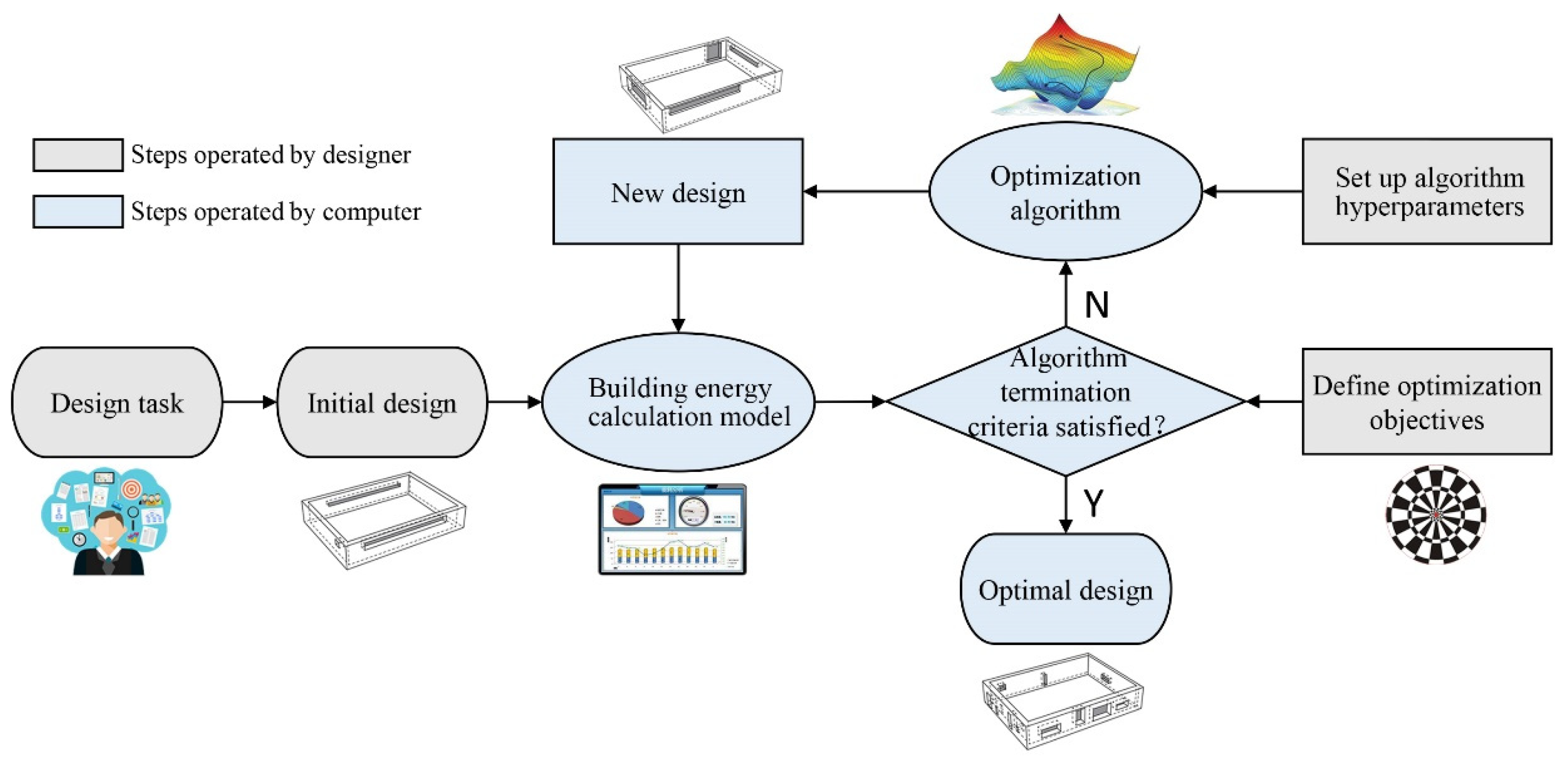
• The proposed metamodel-based methodology for hyperparameter optimization of algorithms in BEO is universal. When a BEO problem arises in which the optimization algorithms applied and the efficacy evaluation criteria of the algorithms concerned differ from those used in this paper, the method illustrated in Figure 3 is also applicable to maximize the efficacy of the algorithm on specific evaluation criteria by optimizing the HPSs of the algorithm.

5.2. Challenges and Future Works

The main challenge with the developed method is to create ANN-trained metamodels of BEO problems, which has a high technical threshold for designers. The future work aims to establish an integrated platform based on the GenOpt software, which will automatically series three technical modules, including metamodeling, algorithm hyperparameter optimization, and the BEO technique. In addition, in order to further explore the HPSs distribution characteristics of algorithms for different BEO problems, more benchmark BEO problems with different properties will be constructed, the hyperparameters of more novel algorithms will be optimized, and the optimal HPSs characteristics of the algorithms will be analyzed based on the data mining technologies.

References

1. IEA. World Energy Statistics and Balances 2018; IEA: Paris, France, 2018. [Google Scholar]
2. Wetter, M.; Wright, J. Comparison of a generalized pattern search and a genetic algorithm optimization method. In Proceedings of the 8th International Building Performance Simulation Association Conference, Eindhoven, The Netherlands, 11–14 August 2003; pp. 1401–1408. [Google Scholar]
3. Barber, K.A.; Krarti, M. A review of optimization based tools for design and control of building energy systems. Renew. Sustain. Energy Rev. 2022, 160, 112359. [Google Scholar] [CrossRef]
4. Tian, Z.; Zhang, X.; Jin, X.; Zhou, X.; Si, B.; Shi, X. Towards adoption of building energy simulation and optimization for passive building design: A survey and a review. Energy Build. 2018, 158, 1306–1316. [Google Scholar] [CrossRef]
5. Shi, X.; Tian, Z.; Chen, W.; Si, B.; Jin, X. A review on building energy efficient design optimization from the perspective of architects. Renew. Sustain. Energy Rev. 2016, 65, 872–884. [Google Scholar] [CrossRef]
6. Chen, X.; Yang, H.; Sun, K. Developing a meta-model for sensitivity analyses and prediction of building performance for passively designed high-rise residential buildings. Appl. Energy 2017, 194, 422–439. [Google Scholar] [CrossRef]
7. Yu, W.; Li, B.; Jia, H.; Zhang, M.; Wang, D. Application of multi-objective genetic algorithm to optimize energy efficiency and thermal comfort in building design. Energy Build. 2015, 88, 135–143. [Google Scholar] [CrossRef]
8. Wright, J.; Alajmi, A. The robustness of genetic algorithms in solving unconstrained building optimization problems. In Proceedings of the 9th IBPSA Conference: Building Simulation, Montréal, QC, Canada, 15–18 September 2005; pp. 1361–1368. [Google Scholar]
9. Delgarm, N.; Sajadi, B.; Kowsary, F.; Delgarm, S. Multi-objective optimization of the building energy performance: A simulation-based approach by means of particle swarm optimization (PSO). Appl. Energy 2016, 170, 293–303. [Google Scholar] [CrossRef]
10. Kim, J.; Hong, T.; Jeong, J.; Koo, C.; Jeong, K. An optimization model for selecting the optimal green systems by considering the thermal comfort and energy consumption. Appl. Energy 2016, 169, 682–695. [Google Scholar] [CrossRef]
11. Eisenhower, B.; O’Neill, Z.; Narayanan, S.; Fonoberov, V.A.; Mezić, I. A methodology for meta-model based optimization in building energy models. Energy Build. 2012, 47, 292–301. [Google Scholar] [CrossRef]
12. Pang, Z.; O’Neill, Z.; Li, Y.; Niu, F. The role of sensitivity analysis in the building performance analysis: A critical review. Energy Build. 2020, 209, 109659. [Google Scholar] [CrossRef]
13. Westermann, P.; Evins, R. Surrogate modelling for sustainable building design—A review. Energy Build. 2019, 198, 170–186. [Google Scholar] [CrossRef]
14. Thrampoulidis, E.; Mavromatidis, G.; Lucchi, A.; Orehounig, K. A machine learning-based surrogate model to approximate optimal building retrofit solutions. Appl. Energy 2021, 281, 116024. [Google Scholar] [CrossRef]
15. Elbeltagi, E.; Wefki, H. Predicting energy consumption for residential buildings using ANN through parametric modeling. Energy Rep. 2021, 7, 2534–2545. [Google Scholar] [CrossRef]
16. Dagdougui, H.; Bagheri, F.; Le, H.; Dessaint, L. Neural network model for short-term and very-short-term load forecasting in district buildings. Energy Build. 2019, 203, 109408. [Google Scholar] [CrossRef]
17. D’Amico, A.; Ciulla, G. An intelligent way to predict the building thermal needs: ANNs and optimization. Expert Syst. Appl. 2022, 191, 116293. [Google Scholar] [CrossRef]
18. Razmi, A.; Rahbar, M.; Bemanian, M. PCA-ANN integrated NSGA-III framework for dormitory building design optimization: Energy efficiency, daylight, and thermal comfort. Appl. Energy 2022, 305, 117828. [Google Scholar] [CrossRef]
19. Prada, A.; Gasparella, A.; Baggio, P. A comparison of three evolutionary algorithms for the optimization of building design. Appl. Mech. Mater. 2019, 887, 140–147. [Google Scholar] [CrossRef]
20. Waibel, C.; Wortmann, T.; Evins, R.; Carmeliet, J. Building energy optimization: An extensive benchmark of global search algorithms. Energy Build. 2019, 187, 218–240. [Google Scholar] [CrossRef]
21. Chegari, B.; Tabaa, M.; Simeu, E.; Moutaouakkil, F.; Medromi, H. Multi-objective optimization of building energy performance and indoor thermal comfort by combining artificial neural networks and metaheuristic algorithms. Energy Build. 2021, 239, 110839. [Google Scholar] [CrossRef]
22. Si, B.; Tian, Z.; Jin, X.; Zhou, X.; Tang, P.; Shi, X. Performance indices and evaluation of algorithms in building energy efficient design optimization. Energy 2016, 114, 100–112. [Google Scholar] [CrossRef]
23. Si, B.; Wang, J.; Yao, X.; Shi, X.; Jin, X.; Zhou, X. Multi-objective optimization design of a complex building based on an artificial neural network and performance evaluation of algorithms. Adv. Eng. Inform. 2019, 40, 93–109. [Google Scholar] [CrossRef]
24. Si, B.; Tian, Z.; Jin, X.; Zhou, X.; Shi, X. Ineffectiveness of optimization algorithms in building energy optimization and possible causes. Renew. Energy 2019, 134, 1295–1306. [Google Scholar] [CrossRef]
25. Hamdy, M.; Nguyen, A.T.; Hensen, J.L. A performance comparison of multi-objective optimization algorithms for solving nearly-zero-energy-building design problems. Energy Build. 2016, 121, 57–71. [Google Scholar] [CrossRef] [Green Version]
26. Yang, M.-D.; Lin, M.-D.; Lin, Y.-H.; Tsai, K.-T. Multiobjective optimization design of green building envelope material using a non-dominated sorting genetic algorithm. Appl. Therm. Eng. 2017, 111, 1255–1264. [Google Scholar] [CrossRef]
27. Chen, X.; Yang, H.; Zhang, W. Simulation-based approach to optimize passively designed buildings: A case study on a typical architectural form in hot and humid climates. Renew. Sustain. Energy Rev. 2018, 82, 1712–1725. [Google Scholar] [CrossRef]
28. Futrell, B.J.; Ozelkan, E.C.; Brentrup, D. Optimizing complex building design for annual daylighting performance and evaluation of optimization algorithms. Energy Build. 2015, 92, 234–245. [Google Scholar] [CrossRef]
29. Ascione, F.; Bianco, N.; De Stasio, C.; Mauro, G.M.; Vanoli, G.P. A new methodology for cost-optimal analysis by means of the multi-objective optimization of building energy performance. Energy Build. 2015, 88, 78–90. [Google Scholar] [CrossRef]
30. Cubukcuoglu, C.; Ekici, B.; Tasgetiren, M.F.; Sariyildiz, S. OPTIMUS: Self-Adaptive Differential Evolution with Ensemble of Mutation Strategies for Grasshopper Algorithmic Modeling. Algorithms 2019, 12, 141. [Google Scholar] [CrossRef] [Green Version]
31. Ramallo-González, A.P.; Coley, D.A. Using self-adaptive optimisation methods to perform sequential optimisation for low-energy building design. Energy Build. 2014, 81, 18–29. [Google Scholar] [CrossRef] [Green Version]
32. Ekici, B.; Chatzikonstantinou, I.; Sariyildiz, S.; Tasgetiren, M.F.; Pan, Q.-K. A multi-objective self-adaptive differential evolution algorithm for conceptual high-rise building design. In Proceedings of the 2016 IEEE Congress on Evolutionary Computation (CEC), Vancouver, BC, Canada, 24–29 July 2016; pp. 2272–2279. [Google Scholar]
33. Si, B.; Tian, Z.; Chen, W.; Jin, X.; Zhou, X.; Shi, X. Performance assessment of algorithms for building energy optimization problems with different properties. Sustainability 2018, 11, 18. [Google Scholar] [CrossRef] [Green Version]
34. Vukadinović, A.; Radosavljević, J.; Đorđević, A.; Protić, M.; Petrović, N. Multi-objective optimization of energy performance for a detached residential building with a sunspace using the NSGA-II genetic algorithm. Sol. Energy 2021, 224, 1426–1444. [Google Scholar] [CrossRef]
35. Ghaderian, M.; Veysi, F. Multi-objective optimization of energy efficiency and thermal comfort in an existing office building using NSGA-II with fitness approximation: A case study. J. Build. Eng. 2021, 41, 102440. [Google Scholar] [CrossRef]
36. Andersson, M.; Bandaru, S.; Ng, A.H.C. Towards optimal algorithmic parameters for simulation-based multi-objective optimization. In Proceedings of the 2016 IEEE Congress on Evolutionary Computation (CEC), Vancouver, BC, Canada, 24–29 July 2016; pp. 5162–5169. [Google Scholar]
37. Torcellini, P.; Deru, M.; Griffith, M.; Benne, K. DOE Commercial Building Benchmark Models. National Renewable Energy Laboratory. 2008. Available online: http://www.nrel.gov/docs/fy08osti/43291.pdf (accessed on 6 January 2023).
38. Fanger, P.O. Thermal Comfort: Analysis and Applications in Environmental Engineering; McGraw-Hill Book Company: New York, NY, USA, 1972; pp. 1–244. [Google Scholar]
39. McKay, M.D. Sensitivity and uncertainty analysis using a statistical sample of input values. In Uncertainty Analysis; Ronen, Y., Ed.; CRC Press: Boca Raton, FL, USA, 1988; pp. 145–186. [Google Scholar]
40. Asadi, E.; Silva, M.G.D.; Antunes, C.H.; Dias, L.; Glicksman, L. Multi-objective optimization for building retrofit: A model using genetic algorithm and artificial neural network and an application. Energy Build. 2014, 81, 444–456. [Google Scholar] [CrossRef]
41. Shahin, M.A.; Maier, H.R.; Jaksa, M.B. Data division for developing neural networks applied to geotechnical engineering. J. Comput. Civ. Eng. 2004, 18, 105–114. [Google Scholar] [CrossRef]
42. Li, L.; Fu, Y.; Fung, J.C.H.; Qu, H.; Lau, A.K. Development of a back-propagation neural network and adaptive grey wolf optimizer algorithm for thermal comfort and energy consumption prediction and optimization. Energy Build. 2021, 253, 111439. [Google Scholar] [CrossRef]
43. Ye, Z.; Kim, M.K. Predicting electricity consumption in a building using an optimized back-propagation and Levenberg–Marquardt back-propagation neural network: Case study of a shopping mall in China. Sustain. Cities Soc. 2018, 42, 176–183. [Google Scholar] [CrossRef]
44. Khayatian, F.; Sarto, L. Application of neural networks for evaluating energy performance certificates of residential buildings. Energy Build. 2016, 125, 45–54. [Google Scholar] [CrossRef]
45. Ascione, F.; Bianco, N.; De Stasio, C.; Mauro, G.M.; Vanoli, G.P. Artificial neural networks to predict energy performance and retrofit scenarios for any member of a building category: A novel approach. Energy 2017, 118, 999–1017. [Google Scholar] [CrossRef]
46. Kheiri, F. A review on optimization methods applied in energy-efficient building geometry and envelope design. Renew. Sustain. Energy Rev. 2018, 92, 897–920. [Google Scholar] [CrossRef]
Figure 1. General workflow of the BEO technique.
Buildings 13 00167 g001
Figure 2. General working mechanism of optimization algorithms.
Buildings 13 00167 g002
Figure 3. Flowchart of the methodology.
Buildings 13 00167 g003
Figure 4. Flowchart of hyperparameter optimization of the test algorithm applied in BEO.
Buildings 13 00167 g004
Figure 5. Architectural schematic views of the benchmark models.
Buildings 13 00167 g005
Figure 6. Sample distribution of benchmark problems with 30 design variables.
Buildings 13 00167 g006
Figure 7. Structure of a three-layer feedforward neural network.
Buildings 13 00167 g007
Figure 8. Identifying the ideal design from the Pareto front based on the WSM.
Buildings 13 00167 g008
Figure 9. Illustration of the differences in the NS when the test algorithms use the optimal HPSs and the default ones.
Buildings 13 00167 g009
Figure 10. Illustration of the differences in the optimal objectives when the test algorithms use the optimal HPSs and the default ones.
Buildings 13 00167 g010