Automatic Modeling for Concrete Compressive Strength Prediction Using Auto-Sklearn
Abstract
:Highlights
- It’s feasible to use AutoML for concrete compressive strength prediction.
- Concrete compressive strength model based on AutoML has stronger robustness than ML.
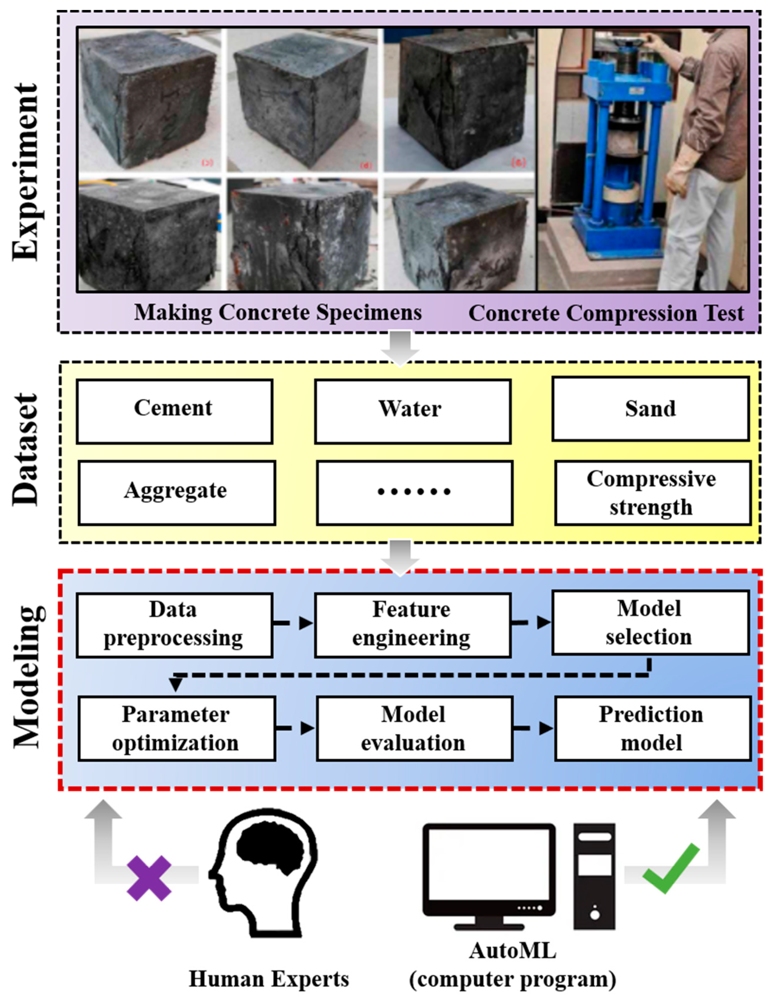
- AutoML can reduce modeling time and reliance upon engineer modeling experience.
Abstract
1. Introduction
- (1)
- We conduct—for the first time in the literature—a feasibility study of AutoML for the prediction of concrete compressive strength.
- (2)
- We obtain a database (containing four types of concrete datasets) from the literature, and we conduct a comprehensive comparison of one AutoML algorithm (i.e., Auto-Sklearn) against five ML algorithms (ANN, SVR, RF, AdaBoost, and XGBoost), to verify the superiority of AutoML over ML.
- (3)
- We verify that Auto-Sklearn can automatically build an accurate concrete compressive strength prediction model without relying on expert experience, and the resulting method is more robust than traditional ML methods.
2. Materials and Methods
2.1. Concrete Database
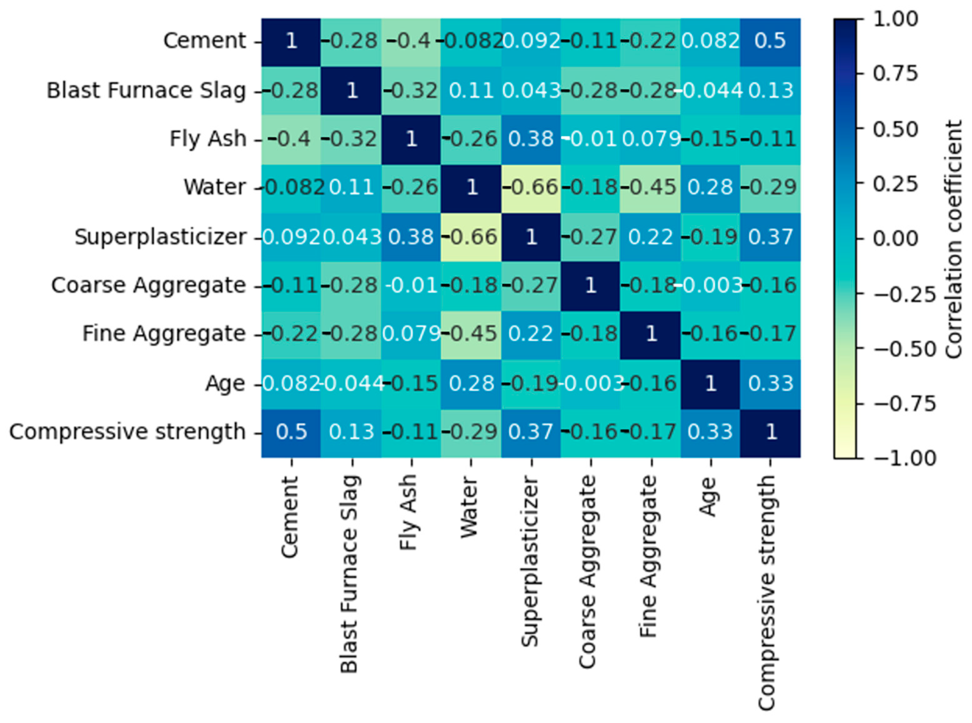
2.1.1. Conventional Concrete Dataset
2.1.2. Rice Husk Ash Concrete Dataset
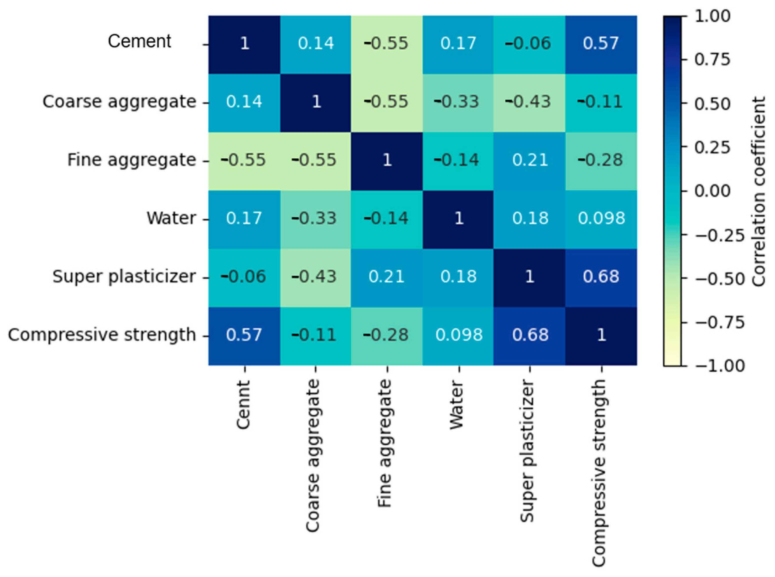
2.1.3. High-Strength Concrete Dataset
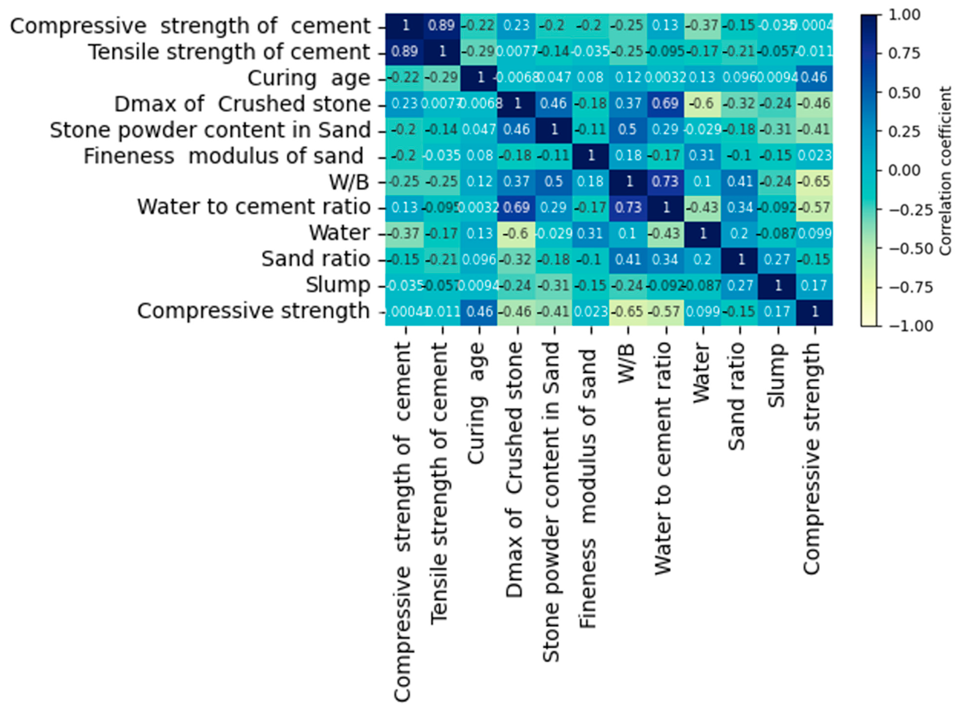
2.1.4. Concrete with Manufactured Sand Dataset
2.2. AutoML Algorithm
2.2.1. Mathematical Model
2.2.2. Auto-Sklearn
2.3. Machine Learning Algorithms
2.3.1. Artificial Neural Network
2.3.2. Support Vector Regression
2.3.3. Random Forest
2.3.4. Adaptive Boosting
2.3.5. Extreme Gradient Boosting
2.4. Performance Evaluation Metrics
2.4.1. Root-Mean-Squared Error
2.4.2. Mean Absolute Error
2.4.3. Coefficient of Determination ()
2.4.4. Mean Absolute Percentage Error
3. Results and Discussion
3.1. Concrete Compressive Strength Prediction Using AutoML
3.2. Prediction of Concrete Compressive Strength Using Machine Learning
3.3. Comparison of Concrete Compressive Strength Prediction Using AutoML and ML
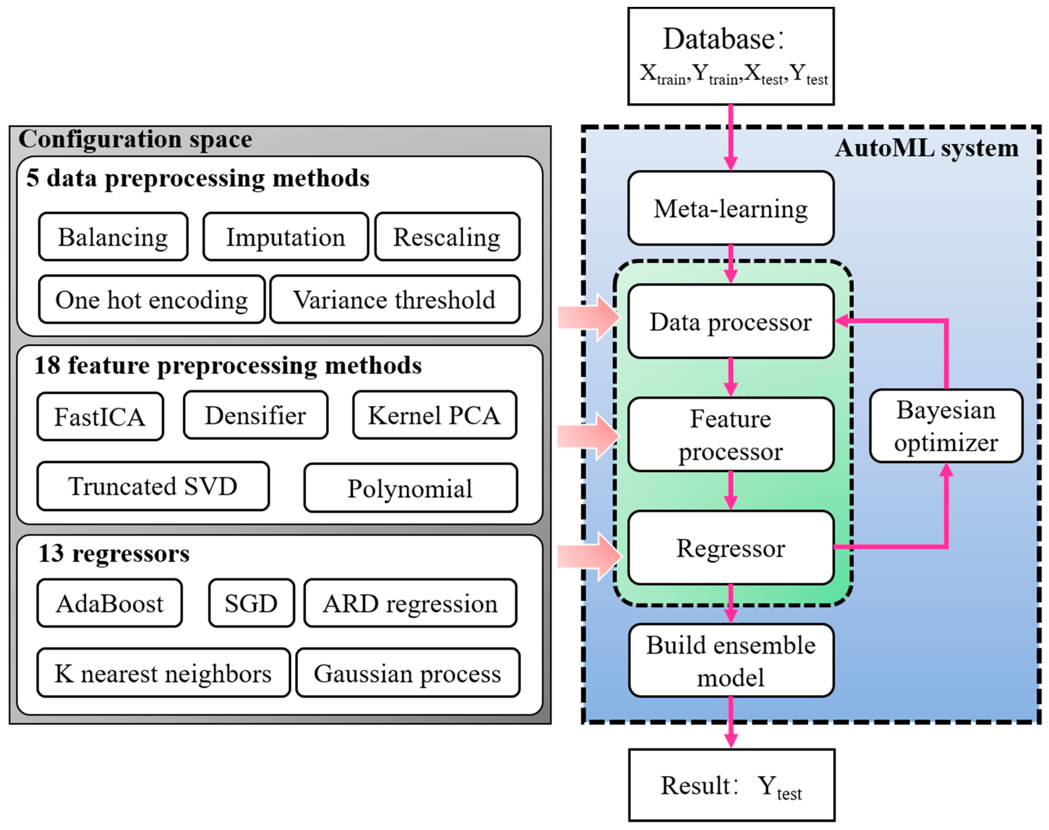
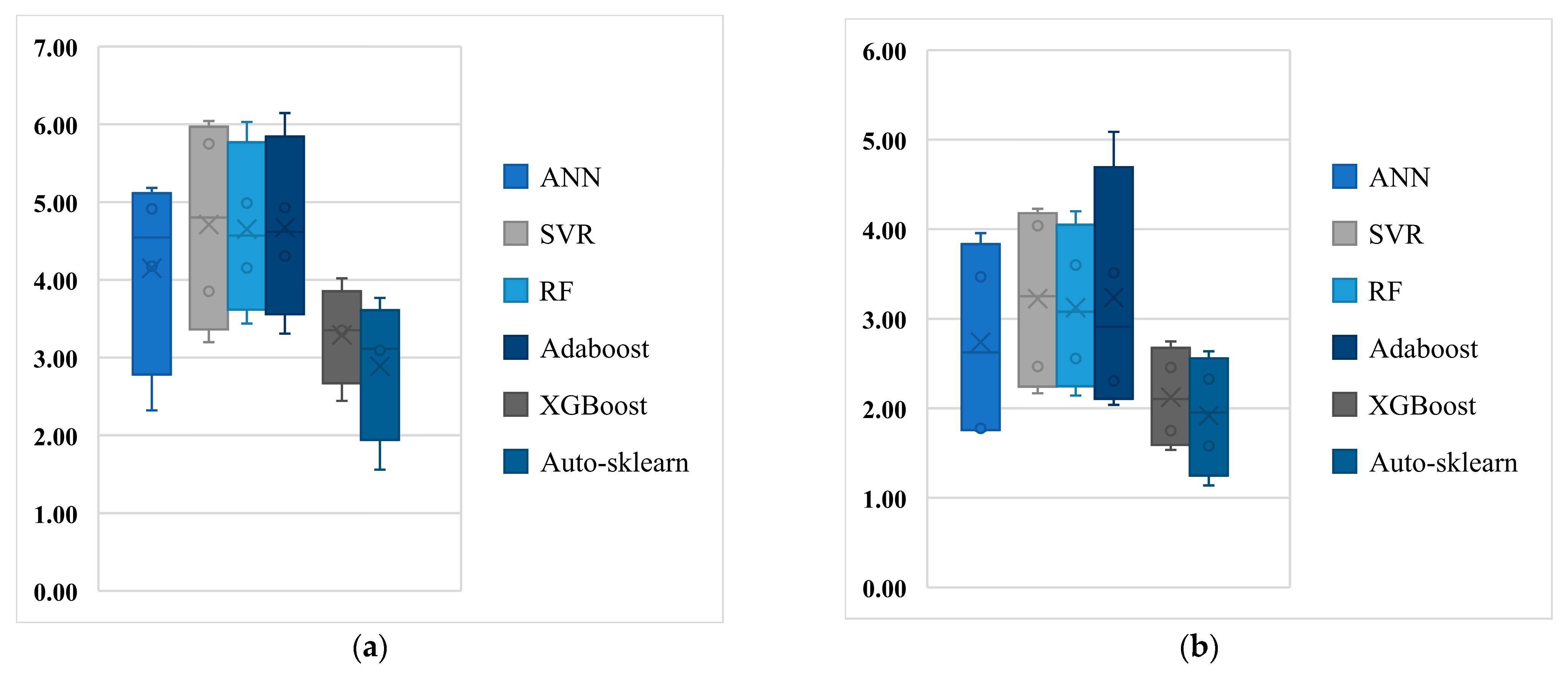
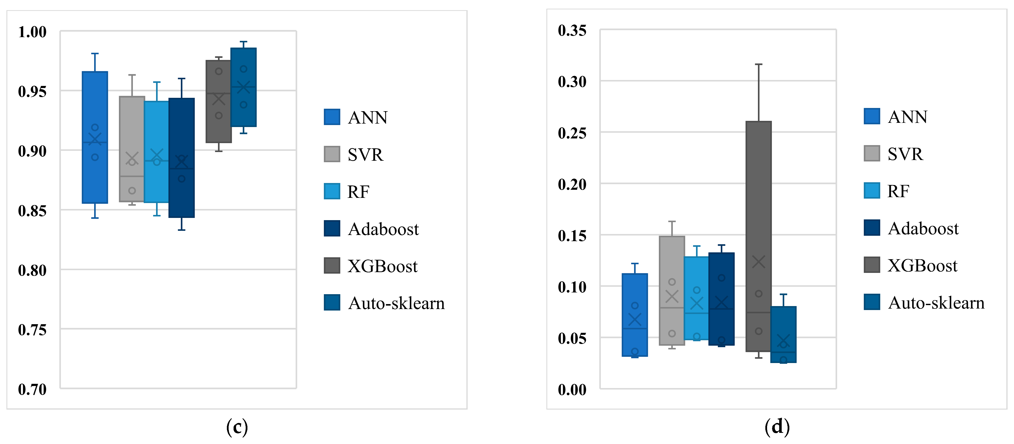
- The accuracy of the Auto-Sklearn algorithm is higher. The multiple algorithm performance metrics presented in Figure 9 show that the Auto-Sklearn algorithm outperforms the five ML algorithms (ANN, SVR, RF, AdaBoost, and XGBoost) on all four datasets. This is because the Auto-Sklearn algorithm can both build complex ensemble models and optimize the entire ML pipeline (including data preprocessing methods, feature preprocessing methods, ML algorithms, and hyperparameters).
- The Auto-Sklearn algorithm is more robust. By comparing the range of the box plot in Figure 9, it can be seen that the fluctuation range of each performance evaluation index of the Auto-Sklearn algorithm (applied to multiple datasets) is significantly smaller than that of the other five ML algorithms. Existing studies have shown that each machine-learning algorithm has a certain scope of application, and there is currently no ML algorithm that performs best on any given dataset [50]. The Auto-Sklearn algorithm can automatically identify the optimal machine-learning pipeline for the dataset in the configuration space and combine them. Therefore, the Auto-Sklearn algorithm is more robust.
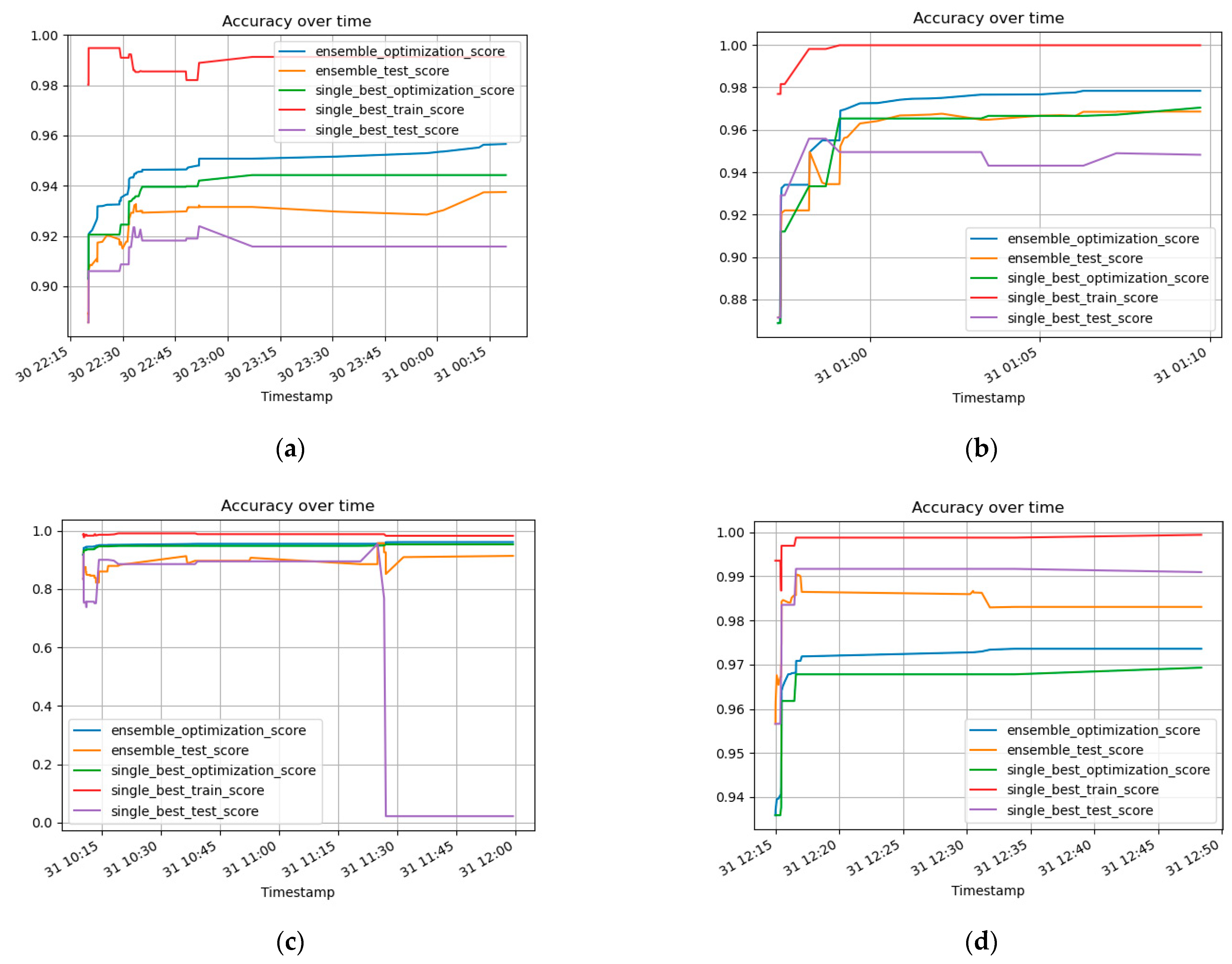
- The Auto-Sklearn algorithm can reduce the modeling time and the dependence on concrete engineer expertise. When building a compressive strength prediction model based on a new concrete dataset, concrete engineers must comprehensively compare multiple ML algorithms and exhaustively optimize the hyperparameters. This results in a considerable time restraint. This study shows that the Auto-Sklearn algorithm can train an accurate concrete compressive strength prediction model within a short time. In addition, once the Auto-Sklearn algorithm is run, there is no need for manual intervention from the concrete engineer, which means that the concrete engineer spends very little time performing modeling. Meanwhile, the automated modeling process means that concrete engineers do not need machine-learning modeling experience and can therefore devote more time to concrete research.
- The Auto-Sklearn algorithm has better scalability. More advanced ML algorithms can be integrated into the configuration space of the Auto-Sklearn algorithm (in particular, numerous ML algorithms that perform well in concrete compressive strength prediction), to satisfy more complex modeling requirements. Traditional ML algorithms can only improve the model performance in a limited manner, by tuning the hyperparameters.
3.4. Comparison with Related Work
- High degree of automation; no reliance upon human experience. To a certain extent, existing research relies upon expert experience to select the hyperparameters. The selection of the hyperparameters is important, but difficult. The present method facilitates automated modeling without relying upon expert experience.
- Stronger robustness. The proposed method achieves accuracies greater than 0.9 (R2) on all datasets, and most of the accuracies approach or exceed those of well-tuned methods in existing studies.
4. Conclusions and Future Work
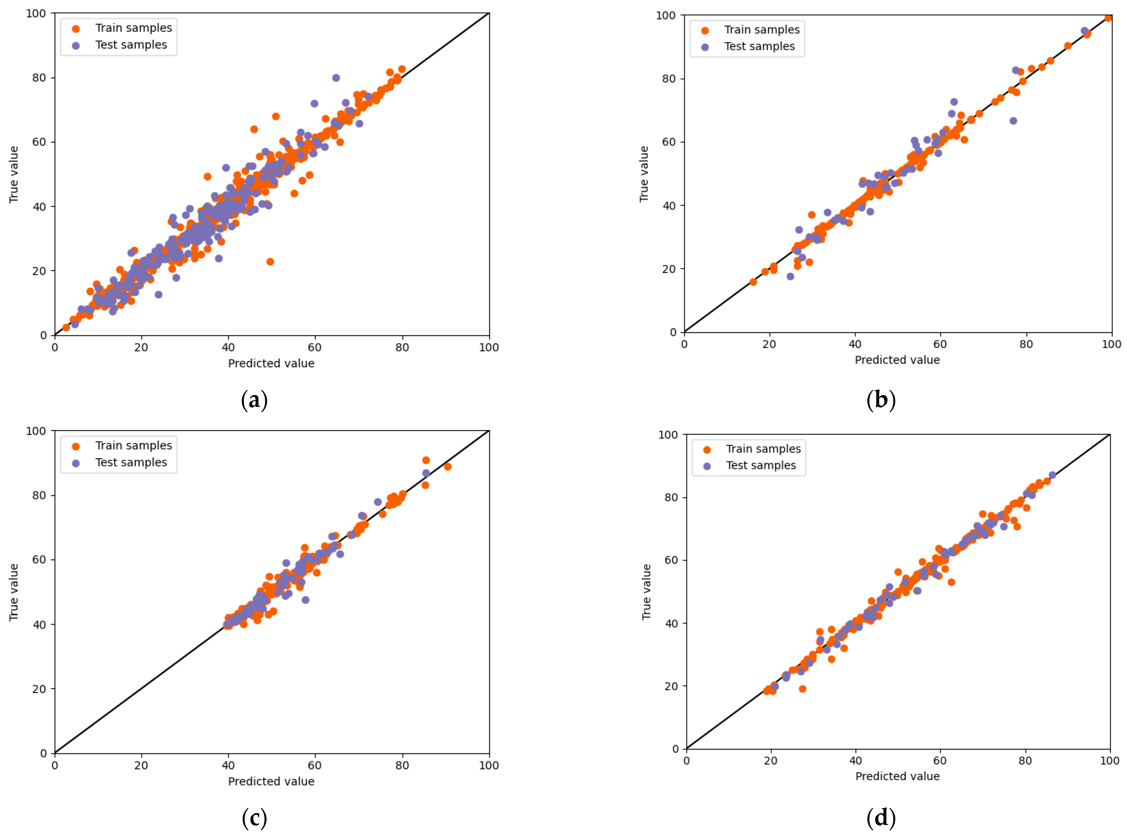
- Auto-Sklearn could automatically build compressive strength prediction models for various types of concrete (CC, RHA, HSC, and MSC).
- The robustness of Auto-Sklearn for different concrete datasets surpassed that of the five ML algorithms (ANN, SVR, RF, AdaBoost, and XGBoost). For all datasets (CC, RHA, HSC, and MSC), Auto-Sklearn achieved the highest (0.938, 0.968, 0.914, 0.991, respectively), and the values of the ML algorithm with adjusted hyperparameters were as follows (where the order CC, RHA, HSC, MSC is adopted): ANN (0.894, 0.931, 0.843, 0.981), SVR (0.854, 0.890, 0.866, 0.963), RF (0.890, 0.892, 0.845, 0.957), AdaBoost (0.893, 0.904, 0.833, 0.960), and XGBoost (0.929, 0.966, 0.899, 0.978). The average of Auto-Sklearn was 0.953, and the average values of the ML models were ANN (0.909), SVR (0.890), RF (0.896), AdaBoost (0.891), and XGBoost (0.943).
- Concrete engineers could use the Auto-Sklearn algorithm to quickly build an accurate concrete compressive strength prediction model, without relying on ML modeling experience; thus, they could devote more time to concrete research.
- More advanced ML algorithms should be integrated in the configuration space, especially those that have a proven superior performance in concrete compressive strength prediction, to further improve the accuracy of AutoML in this task.
- Better optimization methods for ML pipelines should be investigated, to further improve the computational efficiency of AutoML for concrete compressive strength prediction.
Author Contributions
Funding
Institutional Review Board Statement
Informed Consent Statement
Data Availability Statement
Conflicts of Interest
Abbreviations
| AutoML | automated machine learning |
| ML | machine learning |
| LR | linear regression |
| ANN | artificial neural network |
| SVR | support vector regression |
| RF | random forest |
| AdaBoost | adaptive boosting |
| LKRR | Laplacian kernel ridge regression |
| LGBM | light gradient boosting method |
| XGBoost | extreme gradient boosting |
| GB | gradient boosting |
| GEP | gene expression programming |
| RCA | recycled concrete aggregate |
| GGBFS | ground granular blast furnace slag |
| GS | grid search |
| RHA | rice husk ash concrete |
| HSC | high-strength concrete |
| MSC | concrete with manufactured sand |
| CASH | combined algorithm selection and hyperparameter tuning |
| DT | decision tree |
| RMSE | root-mean-squared error |
| MAE | mean absolute error |
| R2 | coefficient of determination |
| MAPE | mean absolute percentage error |
| CC | conventional concrete |
| RHA | rice husk ash concrete |
| HSC | high strength concrete |
| MSC | concrete with manufactured sand |
References
- Das, R.N. High-performance concrete compressive strength’s mean-variance models. J. Mater. Civ. Eng. 2017, 29, 05016003. [Google Scholar] [CrossRef]
- Shah, N.; Mavani, V.; Kumar, V.; Mungule, M.; Iyer, K.K. Impact assessment of plastic strips on compressive strength of concrete. J. Mater. Civ. Eng. 2019, 31, 04019148. [Google Scholar] [CrossRef]
- Kumar Singh, A.; Nigam, M.; Srivastava, R.K. Study of stress profile in cement concrete road of expansive soil due to swell pressure. Mater. Today Proc. 2022, 56, 347–355. [Google Scholar] [CrossRef]
- Ouyang, X.; Wu, Z.; Shan, B.; Chen, Q.; Shi, C. A critical review on compressive behavior and empirical constitutive models of concrete. Constr. Build. Mater. 2022, 323, 126572. [Google Scholar] [CrossRef]
- Kim, K.-M.; Lee, S.; Cho, J.-Y. Influence of friction on the dynamic increase factor of concrete compressive strength in a split Hopkinson pressure bar test. Cem. Concr. Compos. 2022, 129, 104517. [Google Scholar] [CrossRef]
- Cremonez, C.; Maria McCartney da Fonseca, J.; Carolina Seguro Cury, A.; Otto Ferreira, E.; Mazer, W. Analysis of the influence of the type of curing on the axial compressive strength of concrete. Mater. Today Proc. 2022, 58, 1211–1214. [Google Scholar] [CrossRef]
- Miguel Solak, A.; José Tenza-Abril, A.; Eugenia García-Vera, V. Adopting an image analysis method to study the influence of segregation on the compressive strength of lightweight aggregate concretes. Constr. Build. Mater. 2022, 323, 126594. [Google Scholar] [CrossRef]
- Suryanita, R.; Maizir, H.; Zulapriansyah, R.; Subagiono, Y.; Arshad, M.F. The effect of silica fume admixture on the compressive strength of the cellular lightweight concrete. Results Eng. 2022, 14, 100445. [Google Scholar] [CrossRef]
- Benaicha, M.; Burtschell, Y.; Alaoui, A.H. Prediction of compressive strength at early age of concrete–Application of maturity. J. Build. Eng. 2016, 6, 119–125. [Google Scholar] [CrossRef]
- Gong, J.; Wang, Y. Stochastic Development Model for Compressive Strength of Fly Ash High-Strength Concrete. J. Mater. Civ. Eng. 2021, 33, 04021367. [Google Scholar] [CrossRef]
- Quan Tran, V.; Quoc Dang, V.; Si Ho, L. Evaluating compressive strength of concrete made with recycled concrete aggregates using machine learning approach. Constr. Build. Mater. 2022, 323, 126578. [Google Scholar] [CrossRef]
- Wu, Y.; Zhou, Y. Hybrid machine learning model and Shapley additive explanations for compressive strength of sustainable concrete. Constr. Build. Mater. 2022, 330, 127298. [Google Scholar] [CrossRef]
- de-Prado-Gil, J.; Palencia, C.; Silva-Monteiro, N.; Martínez-García, R. To predict the compressive strength of self compacting concrete with recycled aggregates utilizing ensemble machine learning models. Case Stud. Constr. Mater. 2022, 16, e01046. [Google Scholar] [CrossRef]
- Kang, S.; Lloyd, Z.; Kim, T.; Ley, M.T. Predicting the compressive strength of fly ash concrete with the Particle Model. Cem. Concr. Res. 2020, 137, 106218. [Google Scholar] [CrossRef]
- Hwang, K.; Noguchi, T.; Tomosawa, F. Prediction model of compressive strength development of fly-ash concrete. Cem. Concr. Res. 2004, 34, 2269–2276. [Google Scholar] [CrossRef]
- Ren, Q.; Ding, L.; Dai, X.; Jiang, Z.; De Schutter, G. Prediction of compressive strength of concrete with manufactured sand by ensemble classification and regression tree method. J. Mater. Civ. Eng. 2021, 33, 04021135. [Google Scholar] [CrossRef]
- Chen, H.; Yang, J.; Chen, X. A convolution-based deep learning approach for estimating compressive strength of fiber reinforced concrete at elevated temperatures. Constr. Build. Mater. 2021, 313, 125437. [Google Scholar] [CrossRef]
- Yin, X.; Gao, F.; Wu, J.; Huang, X.; Pan, Y.; Liu, Q. Compressive strength prediction of sprayed concrete lining in tunnel engineering using hybrid machine learning techniques. Undergr. Space 2022, 7, 928–943. [Google Scholar] [CrossRef]
- Cook, R.; Lapeyre, J.; Ma, H.; Kumar, A. Prediction of compressive strength of concrete: Critical comparison of performance of a hybrid machine learning model with standalone models. J. Mater. Civ. Eng. 2019, 31, 04019255. [Google Scholar] [CrossRef]
- Dabiri, H.; Kioumarsi, M.; Kheyroddin, A.; Kandiri, A.; Sartipi, F. Compressive strength of concrete with recycled aggregate; a machine learning-based evaluation. Clean. Mater. 2022, 3, 100044. [Google Scholar] [CrossRef]
- Zheng, Z.; Tian, C.; Wei, X.; Zeng, C. Numerical investigation and ANN-based prediction on compressive strength and size effect using the concrete mesoscale concretization model. Case Stud. Constr. Mater. 2022, 16, e01056. [Google Scholar] [CrossRef]
- Mohamed, O.; Kewalramani, M.; Ati, M.; Hawat, W.A. Application of ANN for prediction of chloride penetration resistance and concrete compressive strength. Materialia 2021, 17, 101123. [Google Scholar] [CrossRef]
- Ni, H.-G.; Wang, J.-Z. Prediction of compressive strength of concrete by neural networks. Cem. Concr. Res. 2000, 30, 1245–1250. [Google Scholar] [CrossRef]
- Naderpour, H.; Rafiean, A.H.; Fakharian, P. Compressive strength prediction of environmentally friendly concrete using artificial neural networks. J. Build. Eng. 2018, 16, 213–219. [Google Scholar] [CrossRef]
- Penido, R.E.-K.; da Paixão, R.C.F.; Costa, L.C.B.; Peixoto, R.A.F.; Cury, A.A.; Mendes, J.C. Predicting the compressive strength of steelmaking slag concrete with machine learning–Considerations on developing a mix design tool. Constr. Build. Mater. 2022, 341, 127896. [Google Scholar] [CrossRef]
- Li, H.; Lin, J.; Lei, X.; Wei, T. Compressive strength prediction of basalt fiber reinforced concrete via random forest algorithm. Mater. Today Commun. 2022, 30, 103117. [Google Scholar] [CrossRef]
- Feng, D.-C.; Liu, Z.-T.; Wang, X.-D.; Chen, Y.; Chang, J.-Q.; Wei, D.-F.; Jiang, Z.-M. Machine learning-based compressive strength prediction for concrete: An adaptive boosting approach. Constr. Build. Mater. 2020, 230, 117000. [Google Scholar] [CrossRef]
- Ekanayake, I.U.; Meddage, D.P.P.; Rathnayake, U. A novel approach to explain the black-box nature of machine learning in compressive strength predictions of concrete using Shapley additive explanations (SHAP). Case Stud. Constr. Mater. 2022, 16, e01059. [Google Scholar] [CrossRef]
- Nguyen, H.D.; Truong, G.T.; Shin, M. Development of extreme gradient boosting model for prediction of punching shear resistance of r/c interior slabs. Eng. Struct. 2021, 235, 112067. [Google Scholar] [CrossRef]
- Ma, L.; Zhou, C.; Lee, D.; Zhang, J. Prediction of axial compressive capacity of CFRP-confined concrete-filled steel tubular short columns based on XGBoost algorithm. Eng. Struct. 2022, 260, 114239. [Google Scholar] [CrossRef]
- Nguyen, N.-H.; Abellán-García, J.; Lee, S.; Garcia-Castano, E.; Vo, T.P. Efficient estimating compressive strength of ultra-high performance concrete using XGBoost model. J. Build. Eng. 2022, 52, 104302. [Google Scholar] [CrossRef]
- Li, S.; Richard Liew, J.Y. Experimental and Data-Driven analysis on compressive strength of steel fibre reinforced high strength concrete and mortar at elevated temperature. Constr. Build. Mater. 2022, 341, 127845. [Google Scholar] [CrossRef]
- Imran, H.; Ibrahim, M.; Al-Shoukry, S.; Rustam, F.; Ashraf, I. Latest concrete materials dataset and ensemble prediction model for concrete compressive strength containing RCA and GGBFS materials. Constr. Build. Mater. 2022, 325, 126525. [Google Scholar] [CrossRef]
- Shadbahr, E.; Aminnejad, B.; Lork, A. Determining post-fire residual compressive strength of reinforced concrete shear walls using the BAT algorithm. Structures 2021, 32, 651–661. [Google Scholar] [CrossRef]
- Khorshidi Paji, M.; Gordan, B.; Biklaryan, M.; Armaghani, D.J.; Zhou, J.; Jamshidi, M. Neuro-swarm and neuro-imperialism techniques to investigate the compressive strength of concrete constructed by freshwater and magnetic salty water. Measurement 2021, 182, 109720. [Google Scholar] [CrossRef]
- Zeng, Z.; Zhu, Z.; Yao, W.; Wang, Z.; Wang, C.; Wei, Y.; Wei, Z.; Guan, X. Accurate prediction of concrete compressive strength based on explainable features using deep learning. Constr. Build. Mater. 2022, 329, 127082. [Google Scholar] [CrossRef]
- Tam, V.W.Y.; Butera, A.; Le, K.N.; Silva, L.C.F.D.; Evangelista, A.C.J. A prediction model for compressive strength of CO2 concrete using regression analysis and artificial neural networks. Constr. Build. Mater. 2022, 324, 126689. [Google Scholar] [CrossRef]
- Shahmansouri, A.A.; Yazdani, M.; Ghanbari, S.; Bengar, H.A.; Jafari, A.; Ghatte, H.F. Artificial neural network model to predict the compressive strength of eco-friendly geopolymer concrete incorporating silica fume and natural zeolite. J. Clean. Prod. 2021, 279, 123697. [Google Scholar] [CrossRef]
- Shahmansouri, A.A.; Yazdani, M.; Hosseini, M.; Bengar, H.A.; Ghatte, H.F. The prediction analysis of compressive strength and electrical resistivity of environmentally friendly concrete incorporating natural zeolite using artificial neural network. Constr. Build. Mater. 2022, 317, 125876. [Google Scholar] [CrossRef]
- Asteris, P.G.; Koopialipoor, M.; Armaghani, D.J.; Kotsonis, E.A.; Lourenço, P.B. Prediction of cement-based mortars compressive strength using machine learning techniques. Neural Comput. Appl. 2021, 33, 13089–13121. [Google Scholar] [CrossRef]
- Schwen, L.O.; Schacherer, D.; Geißler, C.; Homeyer, A. Evaluating generic AutoML tools for computational pathology. Inform. Med. Unlocked 2022, 29, 100853. [Google Scholar] [CrossRef]
- He, X.; Zhao, K.; Chu, X. AutoML: A survey of the state-of-the-art. Knowl.-Based Syst. 2021, 212, 106622. [Google Scholar] [CrossRef]
- Atoyebi, O.D.; Modupe, A.E.; Aladegboye, O.J.; Odeyemi, S.V. Dataset of the density, water absorption and compressive strength of lateritic earth moist concrete. Data Brief 2018, 19, 2340–2343. [Google Scholar] [CrossRef]
- Ding, X.; Li, C.; Xu, Y.; Li, F.; Zhao, S. Dataset of long-term compressive strength of concrete with manufactured sand. Data Brief 2016, 6, 959–964. [Google Scholar] [CrossRef] [PubMed]
- Yeh, I.-C. Modeling of strength of high-performance concrete using artificial neural networks. Cem. Concr. Res. 1998, 28, 1797–1808. [Google Scholar] [CrossRef]
- Iftikhar, B.; Alih, S.C.; Vafaei, M.; Elkotb, M.A.; Shutaywi, M.; Javed, M.F.; Deebani, W.; Khan, M.I.; Aslam, F. Predictive modeling of compressive strength of sustainable rice husk ash concrete: Ensemble learner optimization and comparison. J. Clean. Prod. 2022, 348, 131285. [Google Scholar] [CrossRef]
- Farooq, F.; Nasir Amin, M.; Khan, K.; Rehan Sadiq, M.; Faisal Javed, M.; Aslam, F.; Alyousef, R. A Comparative Study of Random Forest and Genetic Engineering Programming for the Prediction of Compressive Strength of High Strength Concrete (HSC). Appl. Sci. 2020, 10, 7330. [Google Scholar] [CrossRef]
- Zhao, S.; Hu, F.; Ding, X.; Zhao, M.; Li, C.; Pei, S. Dataset of tensile strength development of concrete with manufactured sand. Data Brief 2017, 11, 469–472. [Google Scholar] [CrossRef]
- Mu, T.; Wang, H.; Wang, C.; Liang, Z.; Shao, X. Auto-CASH: A meta-learning embedding approach for autonomous classification algorithm selection. Inf. Sci. 2022, 591, 344–364. [Google Scholar] [CrossRef]
- Feurer, M.; Klein, A.; Eggensperger, K.; Springenberg, J.; Blum, M.; Hutter, F. Efficient and robust automated machine learning. Adv. Neural Inf. Process. Syst. 2015, 2, 2755–2763. [Google Scholar]
- Feurer, M.; Eggensperger, K.; Falkner, S.; Lindauer, M.; Hutter, F. Auto-sklearn 2.0: Hands-free automl via meta-learning. arXiv 2020, arXiv:2007.04074. [Google Scholar] [CrossRef]
- Yegnanarayana, B. Artificial Neural Networks; PHI Learning Pvt. Ltd.: Delhi, India, 2009. [Google Scholar]
- Noble, W.S. What is a support vector machine? Nat. Biotechnol. 2006, 24, 1565–1567. [Google Scholar] [CrossRef]
- Belgiu, M.; Drăguţ, L. Random forest in remote sensing: A review of applications and future directions. ISPRS J. Photogramm. Remote Sens. 2016, 114, 24–31. [Google Scholar] [CrossRef]
- Sun, Y.; Liu, Z.; Todorovic, S.; Li, J. Adaptive boosting for SAR automatic target recognition. IEEE Trans. Aerosp. Electron. Syst. 2007, 43, 112–125. [Google Scholar] [CrossRef]
- Chen, T.; Guestrin, C. Xgboost: A scalable tree boosting system. In Proceedings of the 22nd ACM Sigkdd International Conference on Knowledge Discovery and Data Mining, San Francisco, CA, USA, 13–17 August 2016; pp. 785–794. [Google Scholar]
- Chai, T.; Draxler, R.R. Root mean square error (RMSE) or mean absolute error (MAE)?–Arguments against avoiding RMSE in the literature. Geosci. Model Dev. 2014, 7, 1247–1250. [Google Scholar] [CrossRef]
- Willmott, C.J.; Matsuura, K. Advantages of the mean absolute error (MAE) over the root mean square error (RMSE) in assessing average model performance. Clim. Res. 2005, 30, 79–82. [Google Scholar] [CrossRef]
- Edwards, L.J.; Muller, K.E.; Wolfinger, R.D.; Qaqish, B.F.; Schabenberger, O. An R2 statistic for fixed effects in the linear mixed model. Stat. Med. 2008, 27, 6137–6157. [Google Scholar] [CrossRef] [PubMed]
- Tayman, J.; Swanson, D.A. On the validity of MAPE as a measure of population forecast accuracy. Popul. Res. Policy Rev. 1999, 18, 299–322. [Google Scholar] [CrossRef]
- Refaeilzadeh, P.; Tang, L.; Liu, H. Cross-validation. Encycl. Database Syst. 2009, 5, 532–538. [Google Scholar]
- Chou, J.-S.; Chiu, C.-K.; Farfoura, M.; Al-Taharwa, I. Optimizing the prediction accuracy of concrete compressive strength based on a comparison of data-mining techniques. J. Comput. Civ. Eng. 2011, 25, 242–253. [Google Scholar] [CrossRef]

| Ref. | Year | Concrete Type | Size | Parameters | Data Preprocessing Method | Feature Preprocessing Method | Hyperparameter Optimization Method | |
|---|---|---|---|---|---|---|---|---|
| [33] | 2022 | Concrete with RCA and GGBFS | 125 | 5 | None | Human expert | Human expert | LR+RF (0.93) ANN (0.71) SVR (0.56) RF (0.81) |
| [36] | 2022 | Conventional concrete, high-strength concrete, and recycled aggregate concrete | 380 | 9 | Normalized | Human expert | GS | SVM (0.783) ANN (0.939) AdaBoost (0.950) |
| [37] | 2022 | CO2 concrete | 61 | 7 | None | Human expert | Human expert | LR (0.88) ANN (0.95) |
| [32] | 2022 | Steel-fiber-reinforced concrete | 674 | 10 | None | Human expert | GS | SVR (0.684) ANN (0.822) RF (0.851) AdaBoost (0.782) XGBoost (0.886) |
| [11] | 2022 | Recycled and aggregate concrete | 721 | 8 | None | Human expert | Human expert | SVR (0.451) XGBoost (0.850) GB (0.835) |
| Particle swarm optimization | SVR (0.740) XGBoost (0.872) GB (0.875) | |||||||
| [12] | 2022 | Conventional concrete | 559 | 9 | None | Human expert | Human expert | SVR (0.853) |
| GS | SVR (0.931) | |||||||
| [28] | 2022 | Conventional concrete | 1030 | 9 | None | Human expert | GS | XGBoost (0.95) AdaBoost (0.93) LKRR (0.96) LGBM (0.95) |
| [38] | 2021 | Eco-friendly geopolymer concrete | 351 | 5 | None | Human expert | Human expert | ANN (0.960) GEP (0.920) |
| [39] | 2022 | Environmentally friendly concrete | 324 | 7 | None | Human expert | Growing algorithm | ANN (0.993) GEP (0.953) |
| [40] | 2021 | Cement-based mortars | 424 | 6 | None | Sensitivity analysis | Human expert | KNN (0.874) SVM (0.4023) RF (0.9439) DT (0.8526) AdaBoost (0.9473) |
| Type | Variable | Unit | Minimum | Maximum Value | Average Value | Standard Deviation |
|---|---|---|---|---|---|---|
| Independent variable | Cement | kg/m3 | 102.00 | 540.00 | 281.10 | 104.54 |
| Blast furnace slag | kg/m3 | 0.00 | 359.40 | 73.97 | 86.29 | |
| Fly ash | kg/m3 | 0.00 | 200.10 | 54.24 | 64.01 | |
| Water | kg/m3 | 121.80 | 247.00 | 181.55 | 21.35 | |
| Superplasticizer | kg/m3 | 0.00 | 32.20 | 6.21 | 5.97 | |
| Coarse aggregate | kg/m3 | 801.00 | 1145.00 | 972.92 | 77.79 | |
| Fine aggregate | kg/m3 | 594.00 | 992.60 | 773.58 | 80.21 | |
| Age | days | 1.00 | 365.00 | 45.62 | 63.19 | |
| Dependent variable | Compressive strength | MPa | 2.33 | 82.60 | 35.82 | 16.71 |
| Type | Variable | Unit | Minimum | Maximum Value | Average Value | Standard Deviation |
|---|---|---|---|---|---|---|
| Independent variable | Age | days | 1.00 | 90.00 | 34.57 | 33.52 |
| Cement | kg/m3 | 249.00 | 783.00 | 409.02 | 105.47 | |
| Rice husk ash | kg/m3 | 0.00 | 171.00 | 62.33 | 41.55 | |
| Water | kg/m3 | 120.00 | 238.00 | 193.54 | 31.93 | |
| Superplasticizer | kg/m3 | 0.00 | 11.25 | 3.34 | 3.52 | |
| Aggregate | kg/m3 | 1040.00 | 1970.00 | 1621.51 | 267.77 | |
| Dependent variable | Compressive strength | MPa | 16.00 | 104.10 | 48.14 | 17.54 |
| Type | Variable | Unit | Minimum | Maximum Value | Average Value | Standard Deviation |
|---|---|---|---|---|---|---|
| Independent variable | Cement | kg/m3 | 160.00 | 600.00 | 384.35 | 93.01 |
| Coarse aggregate | kg/m3 | 500.00 | 1486.00 | 860.32 | 102.21 | |
| Fine aggregate | kg/m3 | 342.00 | 1135.00 | 806.21 | 113.61 | |
| Water | kg/m3 | 132.00 | 302.08 | 173.57 | 15.56 | |
| Superplasticizer | % | 0.00 | 12.00 | 2.35 | 2.69 | |
| Dependent variable | Compressive strength | MPa | 39.50 | 91.30 | 52.01 | 10.15 |
| Type | Variable | Unit | Minimum | Maximum Value | Average Value | Standard Deviation |
|---|---|---|---|---|---|---|
| Independent variable | Compressive strength of cement | MPa | 38.20 | 55.20 | 48.07 | 3.68 |
| Tensile strength of cement | MPa | 6.90 | 9.10 | 8.22 | 0.48 | |
| Curing age | days | 3.00 | 388.00 | 81.14 | 101.82 | |
| Dmax (maximum grain size) of crushed stone | mm | 20.00 | 80.00 | 31.77 | 12.06 | |
| Stone powder content in sand | % | 0.40 | 20.00 | 8.02 | 4.65 | |
| Fineness modulus of sand | dimensionless | 2.30 | 3.34 | 3.05 | 0.26 | |
| W/B (water–binder ratio) | dimensionless | 0.25 | 0.56 | 0.43 | 0.08 | |
| Water–cement ratio | mw/mc | 0.31 | 0.67 | 0.46 | 0.08 | |
| Water | kg/m3 | 104.00 | 291.00 | 172.69 | 20.76 | |
| Sand ratio | % | 28.00 | 44.00 | 36.69 | 4.27 | |
| Slump | mm | 11.00 | 260.00 | 89.03 | 62.09 | |
| Dependent variable | Compressive strength | MPa | 18.40 | 87.20 | 54.40 | 15.84 |
| Database | No. | Weights | Data Preprocessing Method | Feature Preprocessing Method | Algorithm | Hyperparameters |
|---|---|---|---|---|---|---|
| CC dataset | 1 | 0.22 | None | Feature agglomeration | ANN | 2 hidden layers with 210 neurons |
| 2 | 0.18 | None | Random tree embedding | ANN | 3 hidden layers with 73 neurons | |
| 3 | 0.18 | None | Random tree embedding | ANN | 3 hidden layers with 80 neurons | |
| 4 | 0.12 | None | Feature agglomeration | ANN | 1 hidden layers with 220 neurons | |
| 5 | 0.10 | None | Polynomial | AdaBoost | max depth = 9, estimators = 127, learning rate = 0.07 | |
| 6 | 0.08 | None | Feature agglomeration | ANN | 2 hidden layers with 27 neurons | |
| 7 | 0.04 | None | Feature agglomeration | ANN | 2 hidden layers with 229 neurons | |
| 8 | 0.04 | None | Feature agglomeration | ANN | 3 hidden layers with 252 neurons | |
| 9 | 0.02 | None | Feature agglomeration | AdaBoost | max depth = 8, estimators = 301, learning rate = 0.21 | |
| 10 | 0.02 | None | None | ANN | 2 hidden layers with 189 neurons | |
| RHA dataset | 1 | 0.32 | None | Polynomial | ANN | 2 hidden layers with 261 neurons |
| 2 | 0.18 | None | Polynomial | ANN | 2 hidden layers with 264 neurons | |
| 3 | 0.14 | None | Polynomial | ANN | 3 hidden layers with 257 neurons | |
| 4 | 0.10 | None | Polynomial | ANN | 1 hidden layers with 226 neurons | |
| 5 | 0.10 | None | Polynomial | ANN | 1 hidden layers with 141 neurons | |
| 6 | 0.06 | None | Polynomial | ANN | 2 hidden layers with 257 neurons | |
| 7 | 0.04 | None | Polynomial | ANN | 3 hidden layers with 256 neurons | |
| 8 | 0.04 | None | Polynomial | ANN | 1 hidden layers with 230 neurons | |
| 9 | 0.02 | None | Polynomial | ANN | 1 hidden layers with 226 neurons | |
| HSC dataset | 1 | 0.40 | None | None | ANN | 2 hidden layers with 37 neurons |
| 2 | 0.22 | None | Polynomial | Gaussian process | Alpha = 0.011, thetaL = 4.609 × 10⁻⁷, thetaU =1.02 | |
| 3 | 0.12 | None | Polynomial | Gaussian process | Alpha = 0.011, thetaL = 6.437 × 10⁻⁷, thetaU = 78.86 | |
| 4 | 0.12 | None | Feature agglomeration | ANN | 3 hidden layers with 32 neurons | |
| 5 | 0.10 | None | Feature agglomeration | ANN | 3 hidden layers with 35 neurons | |
| 6 | 0.02 | None | None | Gaussian process | Alpha = 0.011, thetaL = 7.733 × 10⁻⁷, thetaU = 2.796 | |
| 7 | 0.02 | None | Feature agglomeration | ANN | 3 hidden layers with 29 neurons | |
| MSC dataset | 1 | 0.52 | None | Feature agglomeration | Gradient boosting | max leaf nodes = 5, learning rate = 0.08 |
| 2 | 0.18 | None | Feature agglomeration | Gradient boosting | max leaf nodes = 4, learning rate = 0.08 | |
| 3 | 0. 16 | None | Feature agglomeration | Gradient boosting | max leaf nodes = 4, learning rate = 0.08 | |
| 4 | 0.14 | None | Feature agglomeration | Gradient boosting | max leaf nodes = 5, learning rate = 0.02 |
| Database | RMSE | MAE | MAPE | |
|---|---|---|---|---|
| CC dataset | 3.767 | 2.636 | 0.938 | 0.097 |
| RHA dataset | 4.133 | 3.327 | 0.968 | 0.073 |
| HSC dataset | 3.092 | 1.579 | 0.914 | 0.028 |
| MSC dataset | 1.558 | 1.139 | 0.991 | 0.025 |
| Dataset | Algorithm | Hyperparameter | RMSE | MAE | MAPE | |
|---|---|---|---|---|---|---|
| CC dataset | ANN | 3 hidden layers with 231 neurons | 4.914 | 3.469 | 0.894 | 0.122 |
| SVR | C = 417, ε =0.11 | 5.748 | 4.040 | 0.854 | 0.163 | |
| RF | max depth = 14, max features = 3 | 4.987 | 3.601 | 0.890 | 0.139 | |
| AdaBoost | max depth = 10, estimators = 62, learning rate = 0.07 | 4.929 | 3.514 | 0.893 | 0.140 | |
| XGBoost | max depth = 9, learning rate = 0.11 | 4.019 | 2.747 | 0.929 | 0.093 | |
| RHA dataset | ANN | 1 hidden layer with 24 neurons | 4.768 | 3.569 | 0.931 | 0.067 |
| SVR | C = 13, ε = 0.04 | 6.041 | 4.227 | 0.890 | 0.104 | |
| RF | max depth = 10, max features = 7 | 6.029 | 4.200 | 0.892 | 0.096 | |
| AdaBoost | max depth = 9, estimators = 143, learning rate = 1.22 | 5.608 | 4.421 | 0.904 | 0.102 | |
| XGBoost | max depth = 13, learning rate = 0.75 | 3.356 | 2.457 | 0.966 | 0.056 | |
| HSC dataset | ANN | 3 hidden layers with 94 neurons | 4.175 | 1.777 | 0.843 | 0.0305 |
| SVR | C = 440, ε = 0.08 | 3.854 | 2.167 | 0.866 | 0.039 | |
| RF | max depth = 12, max features = 5 | 4.153 | 2.556 | 0.845 | 0.047 | |
| AdaBoost | max depth = 10, estimators = 414, learning rate = 0.03 | 4.305 | 2.305 | 0.833 | 0.041 | |
| XGBoost | max depth = 11, learning rate = 0.02 | 3.35 | 1.75 | 0.899 | 0.03 | |
| MSC dataset | ANN | 2 hidden layers with 35 neurons | 2.320 | 1.749 | 0.981 | 0.036 |
| SVR | C = 195, ε = 0.09 | 3.199 | 2.466 | 0.963 | 0.054 | |
| RF | max depth = 18, max features = 5 | 3.437 | 2.142 | 0.957 | 0.051 | |
| AdaBoost | max depth = 7, estimators = 423, learning rate = 1.70 | 3.309 | 2.039 | 0.960 | 0.048 | |
| XGBoost | max depth = 16, learning rate = 0.90 | 2.443 | 1.536 | 0.978 | 0.316 |
| Dataset | Ref. | Data Preprocessing Method | Feature Preprocessing Method | Hyperparameter Optimization Method | |
|---|---|---|---|---|---|
| CC | [45] | None | None | Human expert | ANN (0.922) |
| [28] | None | Shapley additive explanations | GS | XGBoost (0.95) AdaBoost (0.93) Extra tree (0.94) Decision tree (0.86) LKRR (0.96) LGBM (0.95) | |
| [62] | None | None | Human expert | ANN (0.9025) SVM (0.8836) MART (0.9025) | |
| Present study | Automatic | Automatic | Automatic | Auto-Sklearn (0.938) | |
| RHA | [46] | None | None | Human expert | GEP (0.940) RF (0.913) |
| Present study | Automatic | Automatic | Automatic | Auto-Sklearn (0.938) | |
| HSC | [47] | None | None | Human expert | GEP (0.90) DT (0.90) ANN (0.89) RF (0.96) |
| Present study | Automatic | Automatic | Automatic | Auto-Sklearn (0.914) | |
| MSC | [48] | None | None | None | Fitted formula (0.858) |
| Present study | Automatic | Automatic | Automatic | Auto-Sklearn (0.991) |
Publisher’s Note: MDPI stays neutral with regard to jurisdictional claims in published maps and institutional affiliations. |
© 2022 by the authors. Licensee MDPI, Basel, Switzerland. This article is an open access article distributed under the terms and conditions of the Creative Commons Attribution (CC BY) license (https://creativecommons.org/licenses/by/4.0/).
Share and Cite
Shi, M.; Shen, W. Automatic Modeling for Concrete Compressive Strength Prediction Using Auto-Sklearn. Buildings 2022, 12, 1406. https://doi.org/10.3390/buildings12091406
Shi M, Shen W. Automatic Modeling for Concrete Compressive Strength Prediction Using Auto-Sklearn. Buildings. 2022; 12(9):1406. https://doi.org/10.3390/buildings12091406
Chicago/Turabian StyleShi, M., and Weigang Shen. 2022. "Automatic Modeling for Concrete Compressive Strength Prediction Using Auto-Sklearn" Buildings 12, no. 9: 1406. https://doi.org/10.3390/buildings12091406
APA StyleShi, M., & Shen, W. (2022). Automatic Modeling for Concrete Compressive Strength Prediction Using Auto-Sklearn. Buildings, 12(9), 1406. https://doi.org/10.3390/buildings12091406


