Abstract
The freeze-sealing pipe roof (FSPR) method has been applied to the Gongbei tunnel of the Hongkong–Zhuhai–Macau Bridge, which is the first application of this method in the world. The purpose of the ground-freezing method is soil waterproofing. Temperature is an important indicator for measuring the freezing effect; however, the FSPR method involves unsteady-state conjugate heat transfer between frozen soil, steel pipes, concrete, air, and other media. This paper proposes an unsteady-state conjugate heat transfer model and establishes a global solution algorithm of a strong coupling governing equation based on the virtual density method. Then, a calculation based on COMSOL software is realized and validated. The sensitivity of different factors such as initial formation temperature, different soil layers, and brine temperature on the freezing effect was studied by simulating the FSPR model. It is concluded that the brine temperature had a greater impact on the freezing effect, followed by the soil layer, whereas the formation temperature had the least impact. For muddy silty clay, if the brine temperature is −20 °C, it takes 44 days to meet the design requirements of 2 m. If the brine temperature is −30 °C, 27 days is enough. When the formation temperature is 20 °C, it takes 20 days for medium gravel sand to reach the thickness of the freezing curtain, and 32 days for muddy silty clay. Compared to other soil layers, the freezing effect of the medium gravel sand is relatively better. This research has a certain impetus to similar multimedia freezing heat transfer issues.
1. Introduction
The freeze-sealing pipe roof (FSPR) method is a new type of tunnel construction method combining the artificial ground freezing method with the pipe-roofing method [1]. It was first applied to the Gongbei tunnel of the Hong Kong–Zhuhai–Macao Bridge [2]. Many scholars have studied the FSPR method through theoretical derivation, laboratory experiments, field tests, and numerical simulation [3,4]. Also, some scholars studied the design and construction of the pipe-shed freezing method. However, there is a fundamental difference between pipe-shed freezing and the FSPR method. For the FSPR method, the purpose of the freezing method is soil waterproofing rather than loading, and temperature is an important indicator to measure the freezing state [5]. At present, there are analytical solutions and numerical analysis methods for studying the temperature field. However, the analytical solution must be based on the specific pipe position layout [6], which does not apply to the special pipe position layout of pipe-curtain freezing [7,8]. Because the frozen pipe in the FSPR method is set inside the steel pipe, its heat conduction mode is different from that of the traditional frozen pipe directly contacting the soil. The heat transfer process involves different media such as concrete, steel pipe, soil, air, etc. [9]; thus, the numerical calculation method is more complicated. Relevant scholars have used numerical calculation to analyze the freezing temperature field of the FSPR method [10]. An analytical solution for the temperature field of the FSPR method is based on the Laplace equation boundary conditions for the dislocation arrangement of the single circle pipes [11]. The above research greatly simplifies the model and does not fully consider the heat transfer process between steel pipe, concrete, soil, air, and other media. Therefore, unsteady-state conjugate heat transfer theory is applied to the numerical simulation of the FSPR method [12], which has been applied to the simulation of high-pressure turbines and certain fluid-related parts of aircraft [13]. The term conjugate heat transfer refers to a heat transfer process involving the interaction of heat conduction within a solid body with either the free [14], forced, or mixed convection from its surface to a fluid flowing over it [15]. It finds application in numerous fields, from thermal interaction between surrounding air and fins to thermal interaction between flowing fluid and turbine blades [16,17,18]. At present, there is no freezing simulation of engineering temperature field involving three media such as that of the FSPR structure. Based on the above, this paper takes the FSPR method of the Gongbei tunnel as the research object, proposes an unsteady-state conjugate heat transfer model, establishes a global solution algorithm of a strong coupling governing equation based on the virtual density method that can accurately describe this kind of heat transfer process, and analyzes the sensitivity of the factors such as initial formation temperature, different soil layers, and brine temperature affecting the FSPR effect.
2. Engineering Description of FSPR Method in Gongbei Tunnel
Gongbei Tunnel is the critical link connecting the Hong Kong–Zhuhai–Macao Bridge and Zhuhai [19]. It was constructed with the FSPR method, which is the combination of the pipe-roofing method and artificial ground-freezing method. The layout of the FSPR method is shown in Figure 1 [20]. It is composed of 36 steel jacking pipes with a diameter of 1620 mm and a thickness of 20 mm. Odd-numbered steel pipe jacking is filled with concrete. Even-numbered steel pipe jacking is empty pipes, which are in a staggered layout, and the spacing between pipes is 357 mm. Considering that it is convenient for the overlapping of temporary support during the construction, the two kinds of steel pipe jacking are in staggered layout. The height difference of the circle center is 300 mm, and the buried depth of the tunnel is 4–5 m.
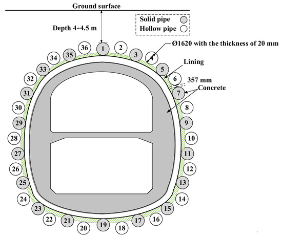
Figure 1.
Layout of pipe roofing.
The construction of Gongbei tunnel consisted of four stages, the pipe jacking stage, the freezing stage, the tunnel excavation stage, and the thawing stage. In the construction stage of the pipe jacking, 36 steel pipes were sequentially jacked into a ring-shaped support system by the pipe jacking machine. In the freezing stage, the low-temperature brine was circulated through the freezing tubes such as the circular freezing tube, the enhancing freezing tube, and the limiting freezing tube, so that the frozen soil reached the designed thickness, forming a waterproofing curtain. The tunnel excavation stage excavated the soil in different areas step by step, and the thawing stage restored the frozen soil to normal temperature soil by circulating high-temperature brine after the excavation was completed.
Considering the calculation efficiency and symmetry of the structure, the typical part of the above-mentioned FSPR was taken as the research object, including solid steel pipe, hollow pipe, and the frozen soil between pipes, as shown in Figure 2.
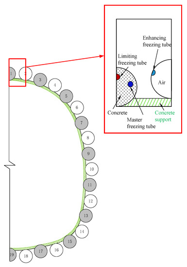
Figure 2.
Local view of FSPR structure.
3. Calculation Model of Unsteady Conjugate Heat Transfer of FSPR Method
3.1. Mathematical Calculation Model
There are three types of freezing tubes in the FSPR method of the Gongbei Tunnel: master freezing tubes with a diameter of 133 mm and thickness of 4 mm, limiting freezing tubes with a diameter of 133 mm and thickness of 4 mm, and enhancing freezing tubes with a diameter of 159 mm and thickness of 4.5 mm. The layout of the freezing tubes is shown in Figure 3.
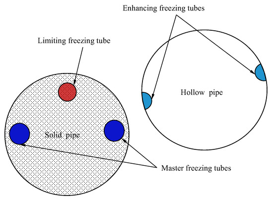
Figure 3.
The layout of freezing tubes.
The freezing phase can be divided into the active freezing phase and the maintainable freezing phase. The construction conditions of the two phases are completely different. In the active freezing phase, the soil below the pipe-roofing has not been excavated, and the model can be simplified into two-dimensions for convenience of calculation, as shown in Figure 4a. In the maintainable freezing phase, the soil in the tunnel has been excavated, the boundary condition is shown in Figure 4b.
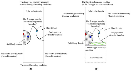
Figure 4.
Calculation model of unsteady-state conjugate heat transfer of FSPR method. (a) Active freezing period. (b) Maintenance freezing period.
The left and right sides of the model are soil. According to the symmetry, it is set as the second-type boundary condition, corresponding to the Neumann boundary condition, which can be expressed as
where is the heat flux value (W/m2), is the thermal conductivity (W/(m∙K)), is the normal direction at the boundary, is the interface, is the temperature (K), and is the time (s).
Since the left and right sides are symmetrical, it is assumed that all heat fluxes passing through the left and right sides are zero.
The upper edge of the model is the surface, which is set as the third-type boundary condition, corresponding to the Robin condition, which can be expressed as
where is the surface heat transfer coefficient (W/(m2∙K)).
The freezing tube is a given temperature boundary, set as the first-type boundary condition, corresponding to the Dirichlet condition, which can be expressed as
The continuity condition of conjugate heat transfer interface is as follows: the conjugate heat transfer interface between soil and air is a steel pipe wall where the continuous conditions of temperature and heat flow shall be met; the expressions are
In Equations (4) and (5), I and II represent the two regions.
In this model, the air is assumed to be laminar. At this time, the heat transfer of the air next to the steel pipe is heat conduction, and the expression for the continuous condition of heat flow is
where is the coefficient of flow heat transfer, is the thermal conductivity of the solid, is the interface temperature, and its expression is
where is the fluid thermal conductivity.
The heat transfer model in the solid adjacent to the interface is heat conduction, and the expression of the heat flow continuity condition is
where is the solid temperature and is the distance between the interface and the center point of the solid unit.
3.2. Governing Equation
3.2.1. Fluid Domain Governing Equation
In this two-dimensional model, air heat transfer is regarded as fluid heat transfer, and the fluid domain control equation is represented by three types of control equations (continuity equation, motion equation, and energy equation) [21,22,23]. The description method adopts the Euler description method. Unless otherwise specified, rectangular coordinates are used to represent Euler coordinates.
The continuity equation is determined according to the Law of Conservation of Mass. In the rectangular coordinate system, the differential form of the continuity equation can be expressed as
where is the fluid density (kg/m3), is the velocity vector (m/s) and its components in the , directions are recorded as , , respectively, and is time. The first term represents the mass increment per unit volume in unit time; the last three items represent the net outflow of mass per unit time and unit volume.
It can be expressed in vector form by using the divergence formula [24]:
To describe the convenience and the simplicity of the motion and energy equations, the concept of the satellite derivative is introduced [25]. Under Euler coordinates, the satellite derivative is more complicated and can be expressed as
where the del operator, also known as the nabla operator [26], and the divergence of the vector is . Then, the continuity equation is expressed by the following derivative:
The motion equation is determined according to the law of momentum balance. The differential form of the motion equation can be expressed as
Similarly, the divergence formula can be used to change Equation (13) into
where the left part is the inertial force of unit volume fluid; the first term on the right is the mass force acting on the unit volume fluid, and the second term is the surface force acting on the unit volume fluid where is the pressure (Pa).
If air, as a fluid with a simple molecular structure, can be regarded as a Newtonian fluid, the expression form of the motion equation will introduce the concept of Generalized Newton’s law to obtain a special form of the motion equation. This equation is called the Navier–Stokes equation, and the expression form is
In which, the left part represents the inertial force per unit volume of fluid, the first term at the right part represents the mass force per unit volume, the second term represents the pressure gradient force acting on the fluid per unit volume, the third term is the viscous deformation stress, and the fourth term is the viscous expansion force.
The expression of the energy conservation equation in thermodynamics is described as the first law of thermodynamics. Taking the rectangular coordinate system as the Euler coordinate system, the energy equation in differential form can be derived as [27]
where represents the heat transferred from radiation unit mass fluid in unit time (W/m3), is the thermal conductivity (W/m·K), and is the internal heating rate (W/m3).
If the air is regarded as ideal air, the energy equation can be expressed as
where is specific heat, which is an ambient-pressure specific-heat meter for fluids here (J/kg·K). At this time, the three basic governing equations—continuity equation, motion equation, and energy equation—constitute the differential equations for solving the fluid domain. When solving the simultaneous equations, it is necessary to introduce the state equation connecting and , and the equations can be solved. The ideal air state equation is
Where is the air constant , is the universal air constant, is 8.31 J/K·mol, is the molar mass, and is 287 J/kg·K for air.
3.2.2. Solid Domain Governing Equation
In this model, the heat conduction of soil and concrete is regarded as solid heat conduction. According to the Law of Energy Conservation and Fourier Law, the differential equation of heat conduction in the solid domain is established as follows:
Generally, when studying the heat transfer in the solid domain, only the heat conduction effect is approximately considered, and phenomena such as the convective heat transfer of a small amount of air and liquid that may be contained in the solid and the resulting water migration are ignored.
3.3. Numerical Implementation of Unsteady-State Conjugate Heat Transfer Model
Through the virtual density method, the global solution algorithm of a strong coupling governing equation is established. The energy equation expressed in physical density is as follows, and the implementation of the algorithm is based on multiphysics module of COMSOL software (Femlab3.2a, Svante Littmarck and Farhad Saeidi, originated from the MATLAB Toolbox, Stockholm, Sweden), which is a coupled tool for solving partial differential equations.
The density in Equation (20) was replaced by to solve the coupling boundary of the steel pipe roof in unsteady-state conjugate heat transfer analysis to solve the problem of heat flux continuity at the coupling interface of steel pipe roof in the analysis of unsteady-state conjugate heat transfer [28,29]. Thus, the strong coupling governing equations’ overall solution algorithm of the unsteady-state conjugate heat transfer model is as follows:
In the process of soil freezing with phase transition, the sensible heat capacity method was used to deal with the problem of soil freezing phase transition [30]. The sensible heat capacity method takes the temperature as the function to be solved and establishes a unified energy equation over the whole region, which is expressed in the form of “Equivalent Specific Heat” [31]. The “Equivalent Specific heat” when the phase transition occurs at a specific temperature Tm is
where is the Dirac function; a sensible heat capacity method model then emerges:
The phase transition of water in the soil freezing process is relatively slow, and it is approximately completed within a certain temperature range. When using the sensible heat capacity method to deal with the phase transition problem of the freezing process, the unfrozen water in the soil must first be removed according to the experimental data. The changes are divided into three sections: the severe phase transition zone, transition zone, and frozen zone. Then, the phase transition is processed by the equivalent specific heat parameter. The equivalent specific heat of the soil area in the energy equation is taken as
where and are the specific heat of thawed soil and frozen soil, J/(kg∙K); is the latent heat of water phase transition, taken as 334,560 J/kg; and are the total water content and ice content of frozen soil; and are the upper and lower boundary temperatures (k) of the phase transition zone of frozen soil. For the convenience of calculation, the temperature is calculated in international Kelvin (k) and described in Celsius (°C).
4. Application of Unsteady Conjugate Heat Transfer Model of FSPR in Gongbei Tunnel
4.1. Assumptions and Calculation Model
The calculation models (a)(b) with a height of 11 m and a width of 6.15 m are shown in Figure 4, and the thickness of both is 1.977 m. In the calculation domain, the cold source freezing pipe wall was regarded as the first temperature boundary, namely the Dirichlet boundary condition, and the refrigerant inlet temperature was taken as the boundary temperature value [32]. When the air pressure is low and the temperature is high, it can be treated as an ideal gas, including the air in the fluid domain. The air in the fluid domain can also be regarded as a compressed fluid and considered as a viscous fluid. At this time, the continuity equation and motion equation (Navier–Stokes equation) are changed [33]. Considering the causes of fluid movement, the flow state of air can be assumed as laminar flow. The continuous condition of heat flux was also treated according to laminar flow in the conjugate heat transfer interface.
According to the above assumptions, the strong coupling general control equations of the calculation model were obtained [34]. The energy equation, ideal gas state equation, continuity equation, and motion equation can be expressed as follows:
In the numerical calculation and analysis, the multiphysics module of COMSOL was used for the secondary development of the software combined with the strong coupling governing equations.
4.2. Soil Mechanics and Thermal Physical Parameters
The soil layer of the Gongbei tunnel mainly includes miscellaneous fill, sludge, mucky silty clay, silty clay, silty sand, medium sand, and gravel sand. The soil layer crossed by tunnel concealed excavation construction is mainly ①, ③-3, ④-3, ⑤-2, ⑤-3, and ⑦-1. According to the test report on physical and mechanical parameters of artificially frozen soil in “Test Report on Physical and Mechanical Parameters of Artificial Frozen Soil at Gongbei Port of Zhuhai Link of Hong Kong-Zhuhai-Macao Bridge” [35], the properties of typical soil layers in Gongbei Tunnel are shown in Table 1, the freezing temperature of the soil is shown in Table 2, and the thermal conductivity of soil is shown in Table 3.

Table 1.
Properties of typical soil layers in Gongbei Tunnel.
Table 2.
The freezing temperature of the soil layer and unfrozen water content at −20 °C.
Table 3.
Thermal conductivity of soil layer (W/(m∙K)).
According to the calculation formula of “Equivalent Specific Heat”, the unfrozen water content in frozen soil is the prerequisite for calculating “Equivalent Specific Heat” [36]. According to the relevant experimental ① conclusions of the Shanghai Yangtze River Tunnel in the same coastal area, the water content of each soil layer at −20 °C was assumed as shown in Table 2, and it was assumed that the phase transition of water in the soil had been completed at −20 °C.
According to the three regions of the phase change of the water in the frozen soil: the severe phase transition zone, transition zone, and freezing zone, each soil layer is divided into four sections from the freezing temperature to −20 °C, combined with the above-unfrozen water content. The specific heat calculation results are listed in Table 4. The values of dynamic viscosity of air at different temperatures are shown in Table 5.
Table 4.
Equivalent Specific Heat of soil layer (J/(kg∙K)).
Table 5.
Dynamic viscosity of air (μPa∙s).
Considering that the change of pressure can be approximately ignored in engineering, the specific heat of air is taken as the specific heat of constant pressure. Its value varies with temperature, thermal conductivity, and specific heat are shown in Table 6. Other material parameters such as steel pipe jacking and filled concrete related to thermal physical parameters are shown in Table 7.
Table 6.
Thermal conductivity of air (W/(m∙K)).
Table 7.
Thermal physical parameters.
4.3. Evaluation Criterion
The parameter value given above are brought into the strong coupling governing equation, and the COMSOL software is used to calculate the freezing state of frozen soil. The numerical model is shown in Figure 4a. There are two evaluation indexes to measure the freezing state, one is the thickness of the frozen soil curtain between steel pipes, and the other is the area of frozen soil, as shown in Figure 5. The cloud graph of the frozen temperature field is obtained as shown in Figure 6. It can be seen that the index of frozen soil develops with the freezing process.
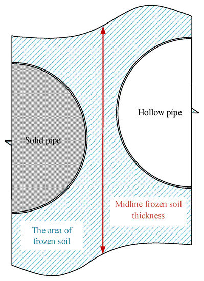
Figure 5.
Evaluation index.
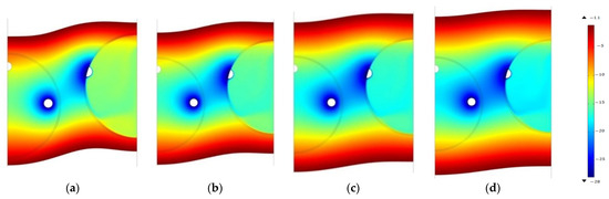
Figure 6.
The freezing temperature distribution: (a) 30 days, (b) 40 days, (c) 50 days, (d) 60 days.
5. Result
Figure 6 is the freezing temperature distribution for 30 days, 40 days, 50 days, and 60 days. When the initial temperature is 20 °C, the model needed to be frozen for 40 days to meet the design requirements of a 2 m thickness of frozen soil curtain between pipes.
Due to the uneven soil quality and uneven frozen soil boundary on the actual project, it is impossible to monitor the actual boundary position of frozen curtain. Therefore, the average thickness of the frozen soil is calculated through the temperature values of monitoring points. According to the field experience of freezing for 40 days to reach a thickness of 2 m, as shown in Figure 6, the model is basically consistent with the numerical simulation results. It is difficult for general methods to obtain such engineering-scale results. The simulation results are reasonable, and the model is validated. Therefore, due to the complexity of site construction conditions, it was necessary to analyze the parameter sensitivity of various factors affecting the freezing effect, such as different initial formation temperatures, different soil layers, and brine temperatures to improve freezing efficiency.
According to the thickness of frozen soil and the area of frozen soil curtain between jacking pipes, the sensitivity of initial formation temperature and different soil layers to the freezing effect was analyzed.
5.1. The Initial Formation Temperature
This analysis took the temperature change and the ground temperature gradient in the formation of Zhuhai City into account. Three different initial temperature conditions of 20 °C, 25 °C, and 30 °C were considered in the calculation model. When the third-type boundary condition was considered, the ambient temperature was the temperature change curve. Temperature change is generally expressed by trigonometric function [37]. The third-type boundary condition with a heat transfer coefficient of 15 W/(m2∙K) was actively frozen for 60 days, and the non-isothermal flow module in COMSOL was used to calculate and compare three different initial temperatures.
As shown in Figure 7, the development of frozen soil thickness between pipe jacking was quite different under different initial temperatures. Similarly, as shown in Figure 8, the development of frozen soil curtain areas is investigated. The difference in frozen soil thickness between pipes under similar initial temperatures for 40 days is about 0.1 m. The freezing duration required for the midline of frozen soil thickness to achieve a representative thickness at different initial temperatures is shown in Table 8. When the initial temperature was 20 °C, the water-sealing path of frozen soil had been completely wrapped with pipe jacking after freezing for 32 days. When the initial temperature was 25 °C, the fully wrapped pipe jacking needed 37 days of freezing, and when the initial temperature was 30 °C, it needed freezing for 40 days.
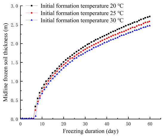
Figure 7.
The thickness of frozen soil between steel pipes.
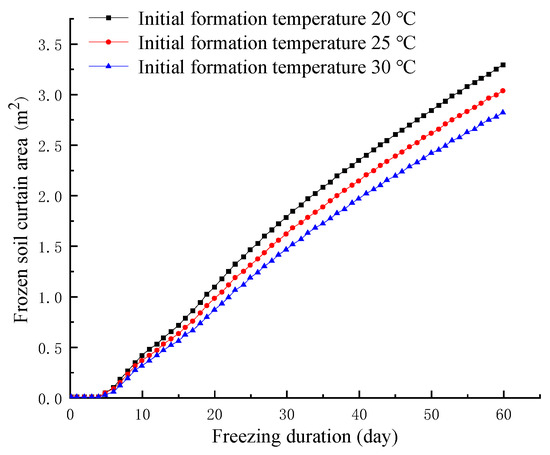
Figure 8.
The area of frozen soil curtain for different initial formation temperature.
Table 8.
Freezing duration of the frozen soil thickness midline at different initial temperatures (day).
As shown in Figure 9, for the development of the average temperature of the frozen soil curtain, after 35 days of freezing (at this time, the thickness of the central frozen soil under the three initial temperatures was about 2 m), the average temperature of the frozen soil was basically about −9 °C. The difference between adjacent cases was less than 0.1 °C, and tended towards consistency with increase in freezing duration. Therefore, in the construction of Gongbei Tunnel by the FSPR method, the initial temperature had a slight influence on the freezing effect. The higher the initial formation temperature, the longer the freezing process needs to last.
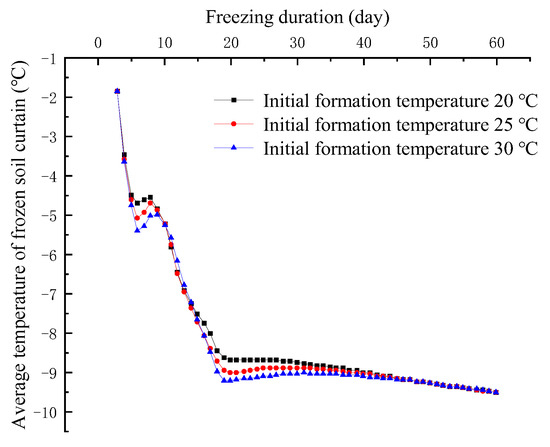
Figure 9.
The average temperature of frozen soil curtain for different initial formation temperature.
5.2. Different Soil Layers
The main soil layers in the FSPR area of Gongbei Tunnel include six kinds of soil layers: ① artificial fill, ③-3 medium gravel sand, ④-3 muddy silty clay, ⑤-2 fine sand, ⑤-3 muddy silty clay, and ⑦-1 sandy cohesive soil. The initial temperature was set at 20 °C, and the surface boundary was set as the third-type boundary condition with a surface heat transfer coefficient of 15 W/(m2∙K). It was actively frozen for 60 days. The non-isothermal flow module in COMSOL was used to calculate and compare the above six soil layers.
As shown in Figure 10, there were considerable differences in the development of frozen soil thickness between pipe jacking of different soil layers, which can be focused on three typical soil layers: ③-3 medium gravel sand, ① artificial fill, ⑤-3 muddy silty clay. The freezing duration required to achieve the midline of pipe jacking of the three layers with representative different thicknesses is shown in Table 9.
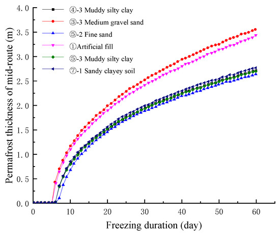
Figure 10.
The thickness of frozen soil between jacking pipes.
Table 9.
The freezing duration required for the frozen soil thickness midline in different soil layers (day).
Correspondingly, the frozen soil curtain area was investigated, as shown in Figure 11. After the ③-3 medium gravel sand was frozen for 20 days, the water sealing path of frozen soil had been completely wrapped by pipe jacking, while the ① artificial fill completely wrapped by pipe jacking needed to be frozen for 22 days to replace the soil. The ⑤-3 muddy silty clay soil layer needed to be frozen for about 32 days.
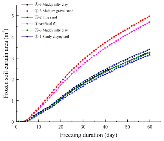
Figure 11.
The area of frozen soil curtain for different soil layers.
As shown in Figure 12, the average temperature of the frozen soil curtain in six soil layers was lower than −8 °C after 20 days of active freezing and reached −10 °C after 60 days of active freezing. Although the average temperature difference of frozen soil in each soil layer was not large enough, there was also a certain difference. Essentially, the difference between soil layers lies in equivalent specific heat and thermal conductivity. When the temperature was −3–−5 °C, the equivalent specific heat of medium gravel sand was only 1810.9 J/(kg∙K), much smaller than other soil layers, and some could reach up to 9454.42 J/(kg∙K). The freezing effect of the medium gravel sand soil was relatively better.
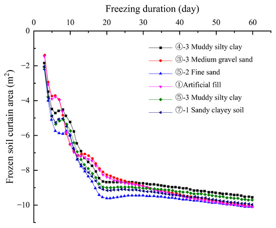
Figure 12.
The average temperature of frozen soil curtain in different soil layers.
In conclusion, all soil layers could meet the freezing effect required by the design with the freezing duration; however, different soil layers have a great impact on the freezing effect. In practical freezing construction, it is necessary to pay more attention to the differences in soil layers and carry out a different freeze scheme design.
5.3. Brine Temperatures in the Freezing Tube
Here, ④-3 muddy silty clay was taken as the calculated soil layer, the initial temperature was set at 20 °C, the active freezing was set for 60 days, and the initial brine temperature pouring into the freezing tube was set at −20 °C, −30 °C, and −40 °C, respectively. The non-isothermal flow module in COMSOL was used to calculate and compare three different brine temperatures. There were significant differences in the midline of frozen soil thickness, as shown in Figure 13. The freezing effect was the best when the brine temperature is −40 °C. It can be seen that the freezing effect was better when the initial temperature of inflow brine in the freezing tube was lower. Therefore, in the case of the buried depth of Gongbei Tunnel, from the perspective of engineering accuracy requirements, it the brine temperature of the freezing tube can be set as low as possible.
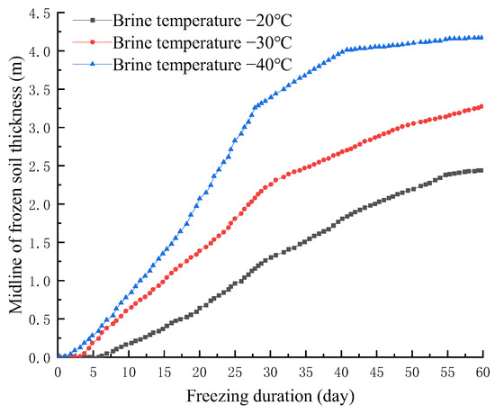
Figure 13.
Thickness of frozen soil in the middle line between pipe jacking.
Table 10 shows the freezing duration required for the midline of pipe jacking to achieve a representative thickness at three different brine temperatures in the freezing tube. If the brine temperature is −20 °C, it will take 44 days to meet the design requirements of 2 m. If the brine temperature is −30 °C, 27 days will be enough. If the brine temperature is −40 °C, then 20 days can meet the requirement.
Table 10.
The freezing duration required in different brine temperatures (day).
Freeze duration depends on freezing intensity and medium. The freezing strength is the cold source, that is, the given brine temperature; the specific heat and thermal conductivity of the medium were directly related to the freezing efficiency, which is the essence of the soil layer difference in this paper.
6. Conclusions
The point of this study is to consider the coupled heat transfer between air and soil. According to the theory of unsteady-state conjugate heat transfer, a complete mathematical model was established to analyze the sensitivity analysis of the calculation parameter to the freezing effect of Gongbei Tunnel.
- (1)
- A mathematical model of unsteady-state conjugate heat transfer based on the FSPR method is established, containing three governing equations in the fluid domain (continuity equation, motion equation, and energy equation), differential equation of heat conduction in the solid domain, and continuity condition of conjugate heat transfer interface. The numerical simulation results verify the rationality of the model.
- (2)
- Through the sensitivity analysis of the factors affecting the freezing effect, it is concluded that the brine temperature has a greater impact on the freezing effect, followed by the soil layer, where the formation temperature has the least impact. For muddy silty clay, if the brine temperature is −20 °C, it takes 44 days to meet the design requirements of 2 m. If the brine temperature is −30 °C, 27 days is enough. When the formation temperature is 20 °C, it takes 20 days for medium gravel sand to reach the thickness of freezing curtain, and 32 days for muddy silty clay. Essentially, the difference between soil layers lies in equivalent specific heat and thermal conductivity. When the temperature is −3~−5 °C, equivalent specific heat of medium gravel sand is only 1810.9 J/(kg∙K), much smaller than other soil layers, and some can reach up to 9454.42 J/(kg∙K). Compared to other soil layers, the freezing effect of the medium gravel sand is relatively better.
- (3)
- In the study, it was found that the initial brine temperature flowing into the freezing pipe would also affect the freezing effect. In engineering practice, the initial temperature in the freezing tube should be controlled reasonably to achieve the best freezing effect without wasting resources and reducing frost heave.
The study provides valuable and operable guidance for practical engineering. However, the model in this study also has some limitations that can be further explored. For example, when establishing the strong coupling general governing equation of unsteady-state conjugate heat transfer, the assumption that the flow state of air is regarded as laminar flow and the assumption that air is approximately regarded as ideal gas still need to be further verified.
Author Contributions
Conceptualization, X.H. and S.S.; methodology, S.D. and S.S.; software, Y.H. and H.L.; validation, Y.H. and H.L.; formal analysis, S.S., F.Z.; resources, X.H.; data curation, Z.H.; writing—original draft preparation, S.S., H.L. and S.D.; writing—review and editing, H.L., S.D. and F.Z.; supervision, S.D. and F.Z. All authors have read and agreed to the published version of the manuscript.
Funding
This research was funded by the National Natural Science Foundation of China (NSFC) (Grant No. 52008208 and 51778287), Natural Science Foundation of Jiangsu Province (Grant No. BK20200707), The Natural Science Foundation of the Jiangsu Higher Education Institutions of China (Grant No. 20KJB560029), China Postdoctoral Science Foundation (Grant No. 2020M671670), Key Laboratory of Soft Soils and Geoenvironmental Engineering (Zhejiang University), Ministry of Education (Grant No. 2020P04), Opening Project of Tunnel and Underground Engineering Research Center of Jiangsu Province (Grant No. 2021SDJJ06).
Institutional Review Board Statement
Not applicable.
Informed Consent Statement
Not applicable.
Data Availability Statement
Not applicable.
Acknowledgments
The funding above is gratefully acknowledged. The author also wishes to thank AL AMIN SARDER at Nanjing Tech University for the language work.
Conflicts of Interest
The authors declare no conflict of interest.
References
- Hu, X.D.; Deng, S.J.; Hui, R. In situ test study on freezing scheme of freeze-sealing pipe roof applied to the Gongbei tunnel in the Hong Kong-Zhuhai-Macau Bridge. Appl. Sci. 2017, 7, 27. [Google Scholar] [CrossRef]
- Li, J.; Li, Z.H.; Hu, X.D. Analysis on Water Sealing Effect of Freezing-sealing Pipe Roof Method. Chin. J. Undergr. Space Eng. 2015, 11, 751–758. [Google Scholar]
- Hu, X.D.; Fang, T. Numerical simulation of temperature field at the active freeze period in tunnel construction using freeze-sealing pipe roof method. In Tunneling and Underground Construction, Proceedings of the Geo-Shanghai 2014 International Conference, Shanghai, China, 26–28 May 2014; Ding, W.Q., Li, X.J., Eds.; American Society of Civil Engineers (ASCE): Houston, TX, USA, 2014; Volume 30, pp. 24–33. [Google Scholar]
- Hu, X.D.; She, S.Y. Study of freezing scheme in freeze-sealing pipe roof method based on numerical simulation of temperature field. In ICPTT 2012: Better Pipeline Infrastructure for a Better Life, Proceedings of the International Conference on Pipelines and Trenchless Technology, Wuhan, China, 19–22 October 2012; Baosong, M., Mohammad, N., Eds.; American Society of Civil Engineers (ASCE): Houston, TX, USA, 2012; Volume 33, pp. 1008–1020. [Google Scholar]
- Duan, Y.; Rong, C.X.; Cheng, H. Model test of pipe curtain freezing temperature field with different pipe jacking combinations. Glacier Frozen Soil 2020, 42, 479–490. [Google Scholar]
- Hu, X.D.; Hong, Z.Q. Analytical solution of steady-state temperature field of special pipe layout form of pipe curtain freezing. Chin. J. Highw. 2018, 31, 113–121. [Google Scholar]
- Hu, X.D.; Deng, S.J.; Wang, Y. Analytical solution to steady-state temperature field with typical freezing tube layout employed in freeze-sealing pipe roof method. Tunn. Undergr. Space Technol. 2018, 79, 336–345. [Google Scholar] [CrossRef]
- Hong, Z.Q.; Hu, X.D.; Fang, T. Analytical solution to steady-state temperature field of Freeze-Sealing Pipe Roof applied to Gongbei tunnel considering operation of limiting tubes. Tunn. Undergr. Space Technol. 2020, 105, 103571. [Google Scholar] [CrossRef]
- Jahangeer, S.; Ramis, M.K.; Jilani, G. Conjugate heat transfer analysis of a heat generating vertical plate. Int. J. Heat Mass Transf. 2007, 50, 85–93. [Google Scholar] [CrossRef]
- Long, W.; Rong, C.X.; Duan, Y. Numerical calculation of temperature field by pipe curtain freezing method in Gongbei tunnel. Coal Geol. Explor. 2020, 48, 160–168. [Google Scholar]
- Afzal, A.; Ansari, Z.; Ramis, M.K. Parallelization of Numerical Conjugate Heat Transfer Analysis in Parallel Plate Channel Using OpenMP. Arab. J. Sci. Eng. 2020, 45, 8981–8997. [Google Scholar] [CrossRef]
- He, L.T.; Oldfieldg, L.M. Unsteady Conjugate Heat Transfer Modeling. J. Turbomach. 2011, 133, 31022. [Google Scholar] [CrossRef]
- Afzal, A.; Samee, A.D.M.; Razak, R.K.A.; Ramis, M.K. Steady and Transient State Analyses on Conjugate Laminar Forced Convection Heat Transfer. Arch. Comput. Methods Eng. 2019, 27, 135–170. [Google Scholar] [CrossRef]
- Samee, A.D.M.; Afzal, A.; Ramis, M.K. Optimal spacing in heat generating parallel plate channel: A conjugate approach. Int. J. Therm. Sci. 2019, 136, 267–277. [Google Scholar] [CrossRef]
- Maffulli, R.; Marinescu, G.; He, L. On the Validity of Scaling Transient Conjugate Heat Transfer Characteristics. J. Eng. Gas Turbines Power 2020, 142, 31021. [Google Scholar] [CrossRef]
- Nouri, M.; Hamila, R.; Perre, P. A double distribution lattice Boltzmann scheme for unsteady Conjugate Heat Transfer: The DD-CHTLB method. Int. J. Heat Mass Transf. 2019, 137, 609–614. [Google Scholar] [CrossRef]
- Voigt, S.; Noll, B.; Aigner, M. Development of a model for unsteady conjugate heat transfer simulations. Prog. Comput. Fluid Dyn. Int. J. 2019, 19, 69–79. [Google Scholar] [CrossRef]
- Makhija, D.S.; Beran, P.S. Concurrent shape and topology optimization for unsteady conjugate heat transfer. Struct. Multidiscip. Optim. 2020, 62, 1275–1297. [Google Scholar] [CrossRef]
- China Communications Second Highway Survey Design and Research Institute. Special Technical Research Report on Gongbei Tunnel of Zhuhai Connection Project of Hongkong-Zhuhai-Macao Bridge; China Communications Second Highway Survey Design and Research Institute Co. Ltd.: Wuhan, China, 2012. [Google Scholar]
- China Communications Second Highway Survey Design and Research Institute. Special Technical Research Report on Gongbei Tunnel of Zhuhai Connection Project of Hongkong-Zhuhai-Macao Bridge Abridged Edition (2013 April); China Communications Second Highway Survey Design and Research Institute Co. Ltd.: Wuhan, China, 2013. [Google Scholar]
- Wang, J. The Application of Computer Simulation of Flow Field in the Design of Heat Treatment Furnace. Ph.D. Thesis, Shanghai Jiao Tong University, Shanghai, China, 2008. [Google Scholar]
- Zhang, L.F. Computational Study on Heat Transfer of Internally Cooled Turbine Blades Using Thermal-Fluid Coupling Method. Master’s Thesis, Northwestern Polytechnical University, Xi’an, China, 2006. [Google Scholar]
- Zhou, G.; Yan, Z.; Xu, S. Fluid Mechanics; Beijing Higher Education Press: Beijing, China, 2000. [Google Scholar]
- Jenkins, R.; Ray, X.; Meyers, R.A. Encyclopedia of Physical Science and Technology, 3rd ed.; Academic Press: Pittsburgh, PA, USA, 2003; pp. 887–902. [Google Scholar]
- Pijush, K.K.; Cohen, I.M.; David, R. Fluid Mechanics, 6th ed.; Academic Press: Pittsburgh, PA, USA, 1981; pp. 109–193. [Google Scholar]
- Shi, T.Z. Narrow del operator and symbolic operation. J. Henan Financ. Univ. 2007, 4, 16–19. [Google Scholar]
- Wang, Q.; Chen, B.Y.; Miao, X.P. Research on Numerical Method of Three-Dimensional Unsteady Coupled Heat Transfer Problem. In The Fourth National Symposium on New Technologies of Refrigeration and Air Conditioning, Proceedings of the Conference of China Refrigeration Society, Nanjing, China, 7–9 April 2006; China Academic Journal Electronic Publishing House: Beijing, China, 2006. [Google Scholar]
- Guo, L.K. Numerical Calculation of Heat Transfer; Anhui Science and Technology Press: Hefei, China, 1987. [Google Scholar]
- Jiang, P.X.; Ke, D.Y.; Ren, Z.P. PHOENICS Solve the Coupled Problem of Unsteady Conduction Convection and Radiation Heat Transfer. J. Tsinghua Univ. 1999, 4, 113–117. [Google Scholar]
- Sugawara, M.; Komatsu, Y.; Beer, H. Melting and freezing around a horizontal cylinder placed in a square cavity. Heat Mass Transf. 2008, 45, 83–92. [Google Scholar] [CrossRef]
- Guo, L.K.; Kong, X.Q.; Chen, S.N. Computational Heat Transfer; University of Science and Technology of China Press: Hefei, China, 1988. [Google Scholar]
- Pimentel, E.; Papakonstantinou, S.; Anagnostou, G. Numerical interpretation of temperature distributions from three ground freezing applications in urban tunnelling. Tunn. Undergr. Space Technol. 2012, 28, 57–69. [Google Scholar] [CrossRef]
- Wang, T.; Zhang, F.; Furtney, J. A review of methods, applications and limitations for incorporating fluid flow in the discrete element method. J. Rock Mech. Geotech. Eng. 2022, 14, 1005–1024. [Google Scholar] [CrossRef]
- Niu, J.; Jiang, L.; Luo, X.; Deng, Z. Structured Method of Dynamic Fully Coupled Rheological Model for Seepage Field and Stress Field in Concrete Dam. In IOP Conference Series Earth and Environmental Science, Proceedings of the 7th International Conference on Environmental Science and Civil Engineering, Seoul, Kerea, 11–13 April 2017; IOP Publishing Ltd.: London, UK, 2021. [Google Scholar]
- Institute of Rock and Soil Mechanics Chinese Academy of Sciences. Experimental Report on the Physical and Mechanical Parameters of Artificially Frozen Soil at the North Port of the Zhuhai Connecting Side Arch of the Hong Kong-Zhuhai-Macao Bridge; Institute of Rock and Soil Mechanics Chinese Academy of Sciences: Wuhan, China, 2012. [Google Scholar]
- Wang, A.; Xie, Z.; Feng, X.; Tian, X.; Qin, P. A soil water and heat transfer model including changes in soil frost and thaw fronts. Sci. Chin. 2014, 57, 1325–1339. [Google Scholar] [CrossRef]
- Zhang, M.; Zhang, J.; Lai, Y. Numerical analysis for critical height of railway embankment in permafrost regions of Qinghai–Tibetan plateau. Cold Reg. Sci. Technol. 2005, 41, 111–120. [Google Scholar] [CrossRef]
Publisher’s Note: MDPI stays neutral with regard to jurisdictional claims in published maps and institutional affiliations. |
© 2022 by the authors. Licensee MDPI, Basel, Switzerland. This article is an open access article distributed under the terms and conditions of the Creative Commons Attribution (CC BY) license (https://creativecommons.org/licenses/by/4.0/).