Abstract
Accurate building models are widely used in the construction industry in the digital era. UAV cameras combined with image-based reconstruction provide a low-cost technology for building modeling. Most existing reconstruction methods operate on point clouds, while massive points reduce computational efficiency, and the accumulated error of point position often distorts building edges. This paper introduces an innovative 3D reconstruction method, Edge3D, that recovers building edges in the form of 3D lines. It employs geometry constraints and progressive screening technology to improve the robustness and precision of line segment matching. An innovative bundle adjustment strategy based on endpoints is designed to reduce the global reprojection error. Edges were tested on challenging real-world image sets, and matching precisions of 96% and 94% were achieved on the two image sets, respectively, with good reconstruction results. The proposed approach reconstructs building edges using a small number of lines instead of massive points, which contributes to the rapid reconstruction of building contour construction and obtaining accurate models, serving as an important foundation for the promotion of construction advancement.
1. Introduction
An up-to-date building model plays an essential role in many engineering management tasks, such as energy simulation [1,2,3,4], site mapping and layout planning [5,6,7], the preventive conservation of historical buildings [8,9,10], and building condition monitoring [11,12,13,14], benefiting from their ability to reflect the actual and real-time state of a building.
Existing 3D building model reconstruction methods can be classified into four groups: tape-based methods, total station-based methods, laser scanning-based methods, and image-based methods [15,16]. The first two methods are time-consuming and labor-intensive, and are therefore are unfeasible for the timely update of building models. Laser scanning-based methods adopt the Light Detection and Ranging (LiDAR) technique to collect spatial building data with high precision. However, the equipment costs are relatively high [17], and often require skilled personnel for operation and data analysis. LiDAR data often contain inaccurate points when encountering spatial discontinuity [18], which causes loss of contour information. Image-based methods serve as a low-cost alternative for laser scanning-based methods [19,20]. Combined with Unmanned Aerial Vehicles (UAVs), which provide an effective means of data collection [5,21,22], image-based methods can efficiently obtain a building’s comprehensive spatial data. In addition, they can capture color information for better visual presentation.
Structure-from-Motion (SfM) is the primary technique employed for image-based reconstruction methods [23]. It recovers the imaging scene and simultaneously estimates the location and orientation of the camera. A typical SfM pipeline consists of five steps: feature extraction, feature matching, camera pose recovery, point cloud generation, and global bundle adjustment. The sparse point cloud and camera poses generated from SfM can support the subsequent Multi-View Stereo (MVS) algorithm [24,25] to produce a dense point cloud (Figure 1).
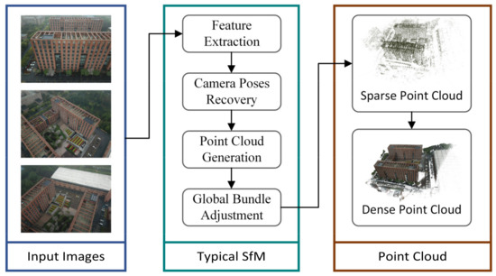
Figure 1.
Typical SfM pipeline.
A point cloud can flexibly depict an object with an irregular shape. However, unlike natural landscapes, a building’s outline is primarily composed of straight-line segments. 3D reconstruction using a typical point-based SfM method often fails to represent the building shape accurately and leads to edge distortions [26,27], as shown in Figure 2. Some scholars have attempted to extract edge points from the point cloud and restore building edges using the detected edge points [20,28,29]. Adopting such an approach can ensure the linearity of the building edge, but the possible absence of the edge points themselves can lead to a reduction in the accuracy of the building edges fitted by them.
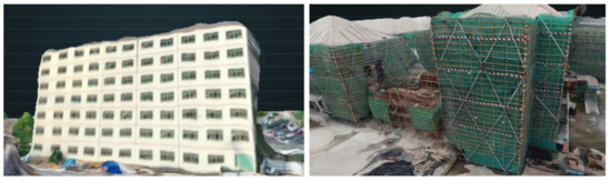
Figure 2.
Distorted building edges.
Operating on feature lines, instead, building edges can be reconstructed with higher integrity, avoiding the distortions caused by the accumulated point error. In addition, as higher dimensional units, a small number of line segments can represent massive points. Adopting 3D lines can reduce the number of features required and further improve the efficiency of reconstruction.
A typical feature line-based reconstruction method requires steps of feature line matching, camera pose recovery, triangulation, and bundle adjustment running for feature lines [30,31]. Significant challenges exist in several respects. First, there is no global geometric constraint to match line segments in adjacent photos, such as the epipolar constraint in point matching [32]. Second, occlusions and line segment detection errors will cause the same 3D line to appear with different lengths in different views [33]. Accordingly, there is no strict endpoint-to-endpoint matching condition for line segments across different views. Third, there is no global linear and minimal parametrization representation for 3D lines to present four degrees of freedom with four parameters [34]. Consequently, bundle adjustment for 3D lines faces the challenge of increased computational costs and instabilities [30].
This paper introduces a feature line-based 3D building reconstruction method, named Edge3D, to recover building edges as 3D lines. As shown in Figure 3, it takes the output of the point-based SfM as input to generate 3D lines representing building edges. The generated 3D lines will help MVS to improve the quality of the final dense point cloud.
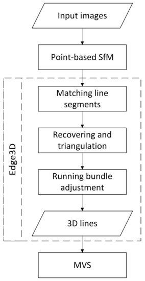
Figure 3.
Workflow illustration.
Edge3D contributes to the method of line-based 3D building reconstruction in three respects:
- The method improves accuracy of feature line matching throughout the workflow. It exploits information from a trifocal tensor, 3D reprojection errors, and line-based bundle adjustment results, in addition to the cue of stereo images;
- The method simplifies the non-linear optimization process by introducing an endpoint-oriented bundle adjustment strategy, which supports a fully automated process for building edge reconstruction in 3D space;
- The method eases the requirement of input images. It introduces the line-level visual neighbor set to search for matches between the input images, including those with a small overlap.
2. Related Works
Most existing line-based reconstruction methods fall into two categories: methods that require matched line segments as input and methods with a complete workflow [35]. The former focus on tasks after line segment matching, such as camera pose recovery and bundle adjustment, assuming that all line segments have been accurately matched. The latter incorporate the line segment matching step to form a complete 3D reconstruction workflow. All included citations are summarized in Table 1.
2.1. Methods Requiring Matched Line Segments
These methods rely on an accurate line segment matching result as their input. Existing line segment matching techniques include texture-based ones and geometry-based ones [32,35,36,37,38,39,40,41,42,43]. The texture-based methods generate distinctive descriptors for each line segment using local texture information, such as color, illumination, and gradient [36,37,38]. Such techniques require a certain quality and quantity of overlaps between corresponding features in different images, which forms a significant challenge to match feature lines [35]. Because of the instability of the texture-based methods, many scholars have attempted to match line segments based on geometry constraints. Wang et al. [39] clustered adjacent line segments into groups and assigned each group a descriptor according to the geometric configuration. Line segment groups in different views were then matched with the descriptor. Similarly, López et al. [40] matched line segment groups based on the context and appearance of adjacent line segments. These methods are suitable for line segment matching in low-texture images. However, the matching accuracy relies heavily on the stability of endpoint recognition, which is usually not guaranteed in various cases. In addition to the local geometry constraint, other types of geometry constraints are also explored for the task. The studies in [35,41,42] employed the epipolar constraint, the coplanarity constraint, and the texture information of the intersection of a line segment pair. The methods were built upon more strict assumptions of the spatial distribution of the lines, thus reducing the generality of the algorithm. The studies in [32,43] adopted the distance invariants between a feature point and a line segment as the determinants. However, the invariants exist only if the feature point and line segment are coplanar in 3D space. Consequently, the applicability of these methods is limited.
Given matched line segments, the line-based reconstruction methods focus on overcoming the challenges of camera pose recovery and bundle adjustment. Compared to point-based methods, a line-based method needs more images and matching groups to recover camera poses. Bartoli and Sturm used triplets of line correspondences for the task [30]. It needs at least 13 triplets of line correspondences to recover the corresponding three-camera poses, and every three images must have a large area of overlap. While a typical method needs at least three images, some scholars have reduced the number to two based on additional constraints. For example, Košecká and Zhang proposed a camera pose recovery method in “Manhattan world”, where 3D lines are in three orthogonal directions [44]. In [45], the relative camera poses between two images can be estimated by three 3D lines, two of which are parallel, and their direction is orthogonal to the third one. These methods reduce the requirement for image overlaps but set a limitation for the distribution of 3D lines in the reconstructed scene.
The challenge of bundle adjustment for lines comes from the mathematic representation of a 3D line. Typically, the representation is linearly overparameterized, such as using the two endpoints or the intersection of two planes, causing difficulties for nonlinear optimization. Aiming at resolving the problem, Bartoli and Sturm [30] proposed a nonlinear orthonormal representation by using only four parameters (i.e., equal to the degrees of freedom of a 3D line) to support nonlinear optimization. Zhang and Peter introduced the Cayley representation that uses minimal parametrization for 3D lines [46]. Both methods designed unique representations and projection functions of 3D lines to overcome the linear overparameterization issue but would increase the complexity of the reconstruction work and affect the practical implementation. These techniques have very few applications [47].
2.2. Methods with a Complete Workflow
It is difficult to obtain a reliable result with matched line segment inputs using the method mentioned above in many scenarios, such as in the case of poorly textured indoor environments or scenes containing wiry structures [48]. Methods with a complete workflow release the restriction of matching data as input. They usually first select a set of possible matching candidates and then filter out mismatched cases phase by phase throughout the whole workflow. For example, Jain et al. introduced a line-based reconstruction method with a set of images and corresponding cameras [49]. Their method did not match line segments directly, but generated a set of hypothetical 3D line segments and verified them by comparing their projection on different views with observed line segments in images. This strategy avoids the impact of inaccurate line segment matching during 3D reconstruction. Still, the hypothetical 3D line segments were continuously and randomly distributed over an extensive range, causing inefficiency in the verification process. Hofer et al. presented a similar approach with a difference of computing possible matches by the epipolar constraint before generating the hypothetical 3D line segments [50]. As a result, their hypothetical 3D line segments were discretely distributed in several possible locations, improving verification efficiency.
In summary, this type of method has better potential for 3D reconstruction. A primary reason is that they can exploit information from multiple stages through the workflow. Information from multiple view geometry, like trifocal tensor, can be derived to improve the reconstruction performance (e.g., [31,49,50]). In comparison, the existing line segment matching methods only use the cues between stereo images.

Table 1.
Summary of related works.
Table 1.
Summary of related works.
| Categories | Subcategories | Description | Source |
|---|---|---|---|
| Methods requiring matched line segment | Line segment matching techniques | Use texture-based or geometry-based cues to match lines in different views. | [32,35,36,37,38,39,40,41,42,43] |
| Camera pose recovery | Restore the camera pose of a photo based on matching line segments. | [30,44,45] | |
| Bundle adjustment | New 3D line representation is used to avoid the overparameterization during global optimization. | [30,46] | |
| Methods with a complete workflow | - | Provide a complete set of reconstruction processes including line segment matching. | [49,50] |
3. Methodology
Edge3D takes raw images, camera poses, and matched points as input to identify building edges through stages of line segment matching, triangulation, and bundle adjustment, as shown in Figure 4. The matching stage determines visual neighbor sets for each feature line by collecting matching candidates with loose geometric constraints. The triangulation stage uses strict constraints to verify the collected candidates for 3D line segment recovery. The bundle adjustment stage minimizes the global error of the 3D line segments and finally obtains a globally optimized output.
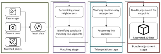
Figure 4.
Edge3D workflow.
3.1. Matching Stage
3.1.1. Determining Visual Neighbor Sets
An image-level visual neighbor set contains images with considerable overlap. Searching for line segments only within a visual neighbor set can significantly improve the efficiency. As shown in Figure 5, Figure 5a,b have many matching line segments and can form a visual neighbor set. On the other hand, Figure 5b,c will not be grouped in the same image-level visual neighbor set by traditional methods. However, there is still a small overlap between them, marked by the red rectangle. Herein we introduce a concept of line-level visual neighbor set. This refers to an image set formed by images sharing the same line segment, even if the line segment is in the corner of an image. Employing the line-level visual neighbor set is better able to use the input images and serve the purpose of line-segment matching.
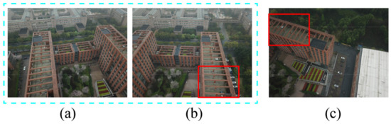
Figure 5.
Drawbacks of image-level visual neighbor set: (a) an aerial photo of the target building; (b) another aerial photo of the target building, and with a large overlap with a; (c) another aerial photo of the target building, and with a small overlap with a and b.
Identifying images sharing the same line segment is the key to building a line-level visual neighbor set. Some scholars have proposed an assumption that adjacent line segments and points on an image have a high chance to co-planarize in 3D space [43,51,52]. Based on this assumption, we use an input-matched point close to a line segment as the reference to find the candidates. In particular, we first build a local region for the target line segment. As shown in Figure 6, a local region is a rectangle centered at the midpoint of the target line segment, whose length is the same as the line segment and the width is . is a user-defined parameter and should be determined according to the shooting distance. The matched feature points within a local region are selected as the reference points for . In Figure 6, and are the reference points while is not. All images possessing a reference point of form a line-level visual neighbor set for . We only need to search for matching line segments in this set in the following steps.
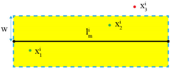
Figure 6.
Local region of line segment .
3.1.2. Identifying Candidates for Matching Line Segments
After defining the visual neighbor sets, we use the epipolar constraint to find matching candidates across different views for each line segment. As shown in Figure 7, the two yellow dotted lines in Figure 7b are the epipolar lines of the endpoints of the target line segments in Figure 7a . in Figure 7b meets the epipolar constraint by having its endpoints located on the epipolar lines, and the other line segments (, , and ) do not.
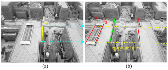
Figure 7.
Epipolar constraint example: (a) yellow solid line is the target line; (b) yellow dotted lines are its corresponding epiplolar lines and other solid lines are the line segments to be judged.
However, due to possible errors of line segment detection, a matching line segment’s endpoints may not be precisely on the epipolar lines. To avoid such false negative cases, we evaluate whether the error is within an acceptable range by
where and are the endpoints of a line segment ; and are the two intersection points between the infinite line corresponding to and two epipolar lines. If is lower than a user-defined threshold , is considered to be a candidate, and otherwise not. As shown in Figure 8, although none of the three line segments strictly meets the epipolar constraint, the errors of and are both within an acceptable range. Therefore, and are persevered as matching candidates and is rejected.
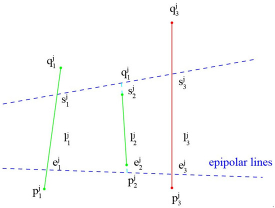
Figure 8.
Epipolar constraint illustration.
In addition, we set a maximum quantity to maintain a manageable number of candidates and computational load for subsequent steps. If there are no more than line segments identified for an image in this step, all of them will be preserved. Otherwise, we rank the line segments by the distances between them and the matching feature point and only pick the top as the candidates. Taking the images in Figure 9 as an example, is one of the reference points for the target line segment in Figure 9a and is the matching feature point for in Figure 9b. It shows that six line segments in Figure 9b satisfy the epipolar constraint. If is set as , the three green line segments closer to are preserved.
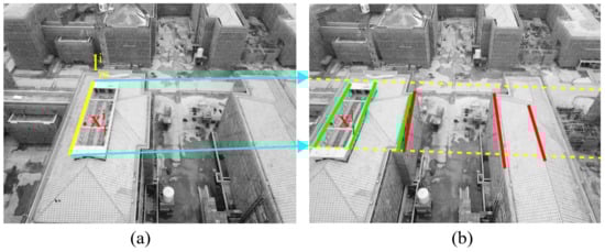
Figure 9.
Ranking candidates: (a) is chosen as reference point; (b) green lines are preserved while red ones are not.
3.2. Triangulation Stage
3.2.1. Verifying Candidates by Reprojection
The candidate set may still contain many mismatching cases. This step employs the trifocal tensor to examine all projected candidates to remove mismatched ones iteratively. As shown in Figure 10, and both belong to the visual neighbor set of the target line segment . The blue line segments in and are the matching candidates for in . Regarding , and the selected candidates from are triangulated to from a hypothetical 3D line . Then, is projected onto another visual neighbor image to form a hypothetical 2D line . The collinearity of with other possible matching line segments in image (e.g., ) is calculated to determine if they are the same line segment. The collinearity can be defined as
where is the angular collinearity and is the position collinearity between the hypothesis 2D line and candidate ; is the angle between and ; is the midpoint of ; is the distance between and . and are user-defined parameters to determine the collinearity. If is not greater than , we consider their angular collinearity holds. If is not greater than , we consider their position collinearity holds. and are co-linear only if the angular collinearity and the position collinearity both hold.
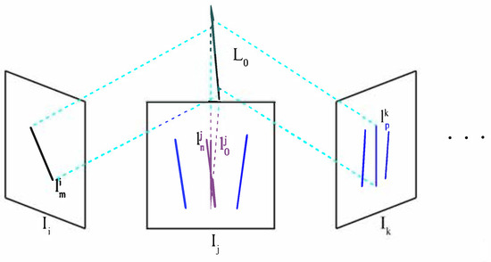
Figure 10.
Reprojection to remove mismatched line segments.
After measuring all the candidates, there are three possible scenarios. Figure 11 illustrates the cases with the red line segment being the hypothetical line segment, the green line segments being the accepted ones, and the blue line segments being the rejected ones. In the first scenario in Figure 11a, there is only one line segment satisfying the condition. We accept it as the true matching line segment for the hypothetical 3D line. If no line segment satisfies the condition, as shown in Figure 11b, we reject them all. If more than one line segment satisfies the collinearity, as shown in Figure 11c, there is a high possibility that these line segments are very close to each other in the image. Considering inevitable camera pose errors, selecting anyone of them as the true matching line segment would be risky. To avoid interference introduced by this situation, all candidates are rejected. This strategy may affect the recall rate but significantly improve the matching precision. Section 4 discusses this situation with more details.
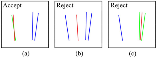
Figure 11.
Three measurement scenarios: (a) only one line segment satisfies the collinearity; (b) no line segment satisfies the collinearity; (c) more than one line segment satisfies the collinearity.
The above process continues until it traverses all images in the visual neighbor set. When there are at least a certain number (e.g., four in this study) of line segments that can be projected onto , is considered a true 3D line and all the matching line segments are stored as a matching group. If not, another line segment is selected to form a new hypothetical 3D line with and the steps are repeated.
3.2.2. Recovering Line Segments
The above steps have produced groups of matching line segments and corresponding 3D lines. Since the bundle adjustment must be operated on 3D line segments, we need to convert these 3D lines into 3D line segments. A 3D line segment often appears with different lengths in different views. Therefore, this step recovers its 2D line segments simultaneously to assist in the conversion.
First, we recover the line segment in by taking the union of and the projected line segments from and , as shown in Figure 12a. Second, we project the recovered line segment from back to , then take the union of the projected line segment and to recover the line segments in . The recovery on follows the same procedure, as shown in Figure 12b. The recovered line segment on each image should have its entire length to this step.
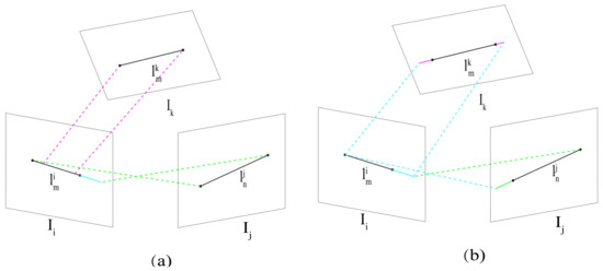
Figure 12.
Recovering line segments on a 2D plane: (a) is recovered by other two line segments; (b) other two line segments are recovered by .
3.3. Bundle Adjustment Stage
The bundle adjustment stage minimizes the 2D observation errors of the line segments obtained from the triangulation stage. A common optimization strategy is to treat a 3D line segment as a 3D line and reduce the reprojection error between the projected line and the observed line segment. The advantage is that it can avoid the interference brought by the instability of endpoint recovery during optimization. The downside is that it would increase the complexity of the process. Such a strategy requires a unique design of mathematical representation and projection equation for 3D lines to optimize points, lines, and camera poses simultaneously. It significantly limits the implementation in practice. Moreover, camera poses have been optimized by mature point-based bundle adjustment methods in previous steps; it can hardly be improved any further through the line-based bundle adjustment.
Our method adopts a different strategy of conducting bundle adjustment only for line segments. Since there are mature point-based methods (e.g., COLMAP [53], VisualSFM [54]) for deriving camera poses, we use input camera poses to recover the endpoints of lines and consider each line segment as the target object for optimization. By minimizing the reprojection error between the projected endpoints and the observed endpoints, we can improve the position accuracy of a 3D line segment. Such a strategy can fully use the point-based bundle adjustment results and alleviate the hassle of additional design for 3D line optimization. The reprojection error function is defined as
where is the camera matrix corresponding to image ; projects the endpoints of 3D line onto image ; computes the Euclidean distance between the projected endpoints and the observed endpoints of as the reprojection error; is a loss function to reduce the interference from outliers. If the reprojection error is greater than a user defined threshold , the corresponding line segment will be removed from the matching group. After removing the mismatched line segments, if there are still no less than three line segments remaining in a matching group, we accept it as the final matching group. If there are fewer than three line segments left, this group will be rejected. The matching precision can be further improved through this step.
4. Case Illustration and Discussion
We tested our method on challenging real-world images. The target was an office building with significant linearity. A total of 124 drone images of the whole building were taken from different perspectives at a distance of around 100 m (Figure 13). Additionally, 168 drone images of one of the building’s walls were taken from different perspectives from a distance of around 50 m (Figure 14). Testing images with different shooting distances were used to comprehensively evaluate the reconstruction effect.
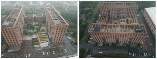
Figure 13.
Drone images of the building image set.
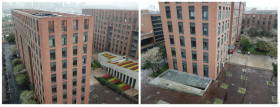
Figure 14.
Drone images of the wall image set.
The parameters were determined by trial and error as follows: the local region width pixels, the collinearity requirement and pixels, and the maximum quantity . The threshold was defined as four times the 95% confidence coefficient of the reprojection error and the values vary for different image sets.
4.1. Line Segment Matching Results after Each Stage
To demonstrate the improvement of matching accuracy after each stage, we randomly selected a set of images from each of the two image sets for examination. The matching results are illustrated in Figure 15, Figure 16, Figure 17 and Figure 18. The correctly matched line segments are labeled in green, and the mismatched ones are labeled in red.
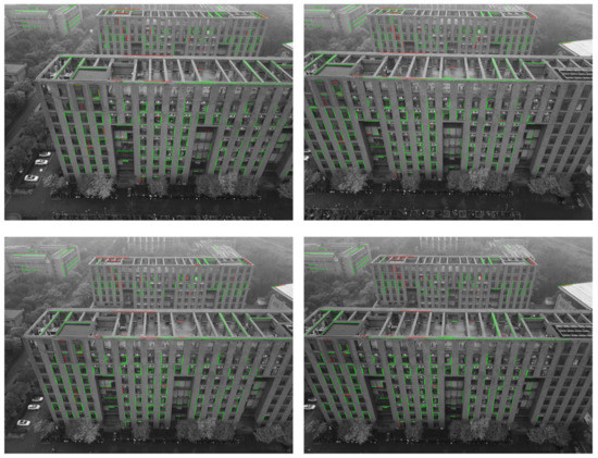
Figure 15.
Matching precision of the building image set after triangulation.
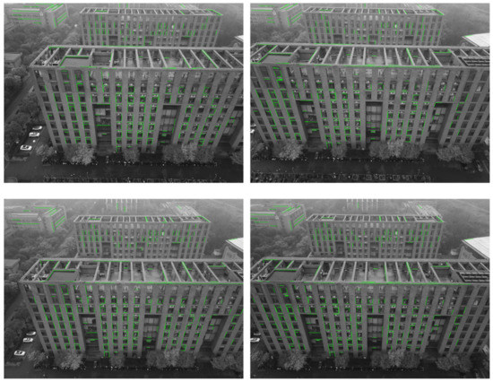
Figure 16.
Matching precision of the building image set after bundle adjustment.
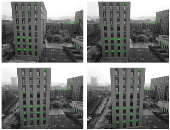
Figure 17.
Matching precision of the building image set after triangulation.
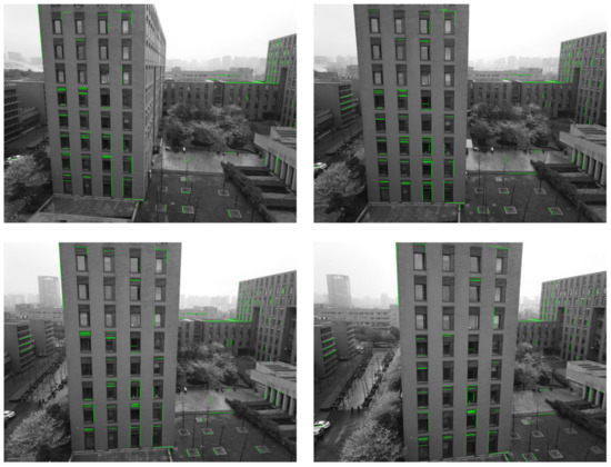
Figure 18.
Matching precision of the wall image set after bundle adjustment.
The corresponding statistical results are shown in Table 2. The matching accuracy was quantitatively evaluated using the value of precision, which was calculated as follows:
where (true positive) is the number of correctly matched line segments; (false positive) is the number of falsely matched line segments. As shown in Table 2, good scores of matching precision (91% and 89%) were achieved for both image sets after the triangulation stage. They were further enhanced (96% and 94%) after bundle adjustment.
Table 2.
Statistical results of the matching accuracy.
In comparison, the matching precision of the wall image set was slightly lower, mainly due to the noise introduced by the line distribution pattern of the images. There are too many line segments close to each other that form clusters in the wall images, for example, the window, the blinds, and the surface texture of the wall. The building images, on the other hand, have most of the line segments sparsely distributed, leading to better effectiveness and precision of selecting matched line segments.
Besides precision, recall is another important metric for evaluating the method, which was calculated as follows:
where (false negative) is the number of falsely rejected line segments. Recall reflects the effectiveness of the algorithm and the richness of the edges in the final reconstructed scene. The results of recall are shown in Figure 19, Figure 20, Figure 21 and Figure 22. Successfully matched line segments are labeled in green, while line segments reserved in the previous stage but failed matching in the current stage are labeled in red.
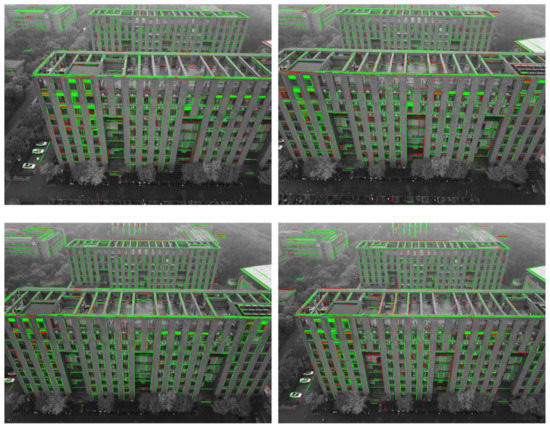
Figure 19.
Matching recall of the building image set after triangulation.
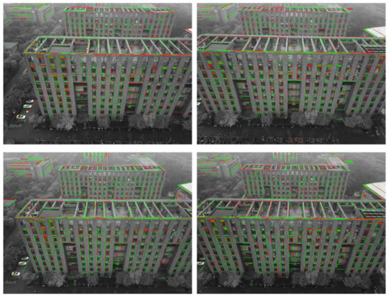
Figure 20.
Matching recall of the building image set after bundle adjustment.
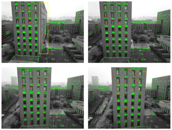
Figure 21.
Matching recall of the wall image set after triangulation.
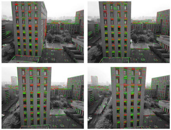
Figure 22.
Matching recall of the wall image set after bundle adjustment.
Table 3 shows the statistical results, whereby the recall values decline after each stage. Recall and precision are usually complementary. Adopting a stricter constraint can reduce and increase precision but may also increase and reduce recall, and vice versa. In this case, a stricter constraint that increases the precision may lead to the rejection of more matching candidates and a lower recall. Besides, some noises introduced by unintentionally captured objects will also decrease the value of recall. As shown in Figure 21, the adjacent wall marked within the yellow rectangle was captured. It rarely appears in other images of the wall image set. Consequently, there are very few matching line segments for it.
Table 3.
Statistical results of the matching recall.
It should be noted that the primary objective of our method is to improve the model quality by reconstructing as many accurate line segments as possible. Precision takes precedence over other metrics. In addition, increasing the number of images can compensate for the decrease in recall.
4.2. Reconstruction Results
The final reconstruction results of the building are shown in Figure 23. The building in the middle is our main reconstruction target. The profile of the building was successfully reconstructed. Some building details, such as the windows and the texture lines of the roof, were also preserved. In comparison, the building roof was better reconstructed than the building façade. As shown in Figure 23, the building roof was presented in significant detail, while the building façade was missing some edges. The main reason for this phenomenon might be the shooting angle of the UAV. While taking pictures, the UAV was often above the building, and captured more details of the building roof than of the building façade. Increasing the number of building façade images would effectively solve this problem.
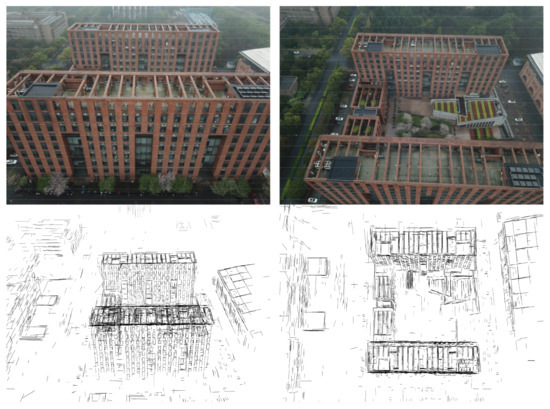
Figure 23.
Reconstruction result of the building image set.
The reconstruction results of the wall image set are shown in Figure 24. The edges of the target wall were reconstructed in detail, and many edges of the adjacent wall marked in the rectangle were also reconstructed. The adjacent wall appears only in around 30 images without significant overlap in the wall image set. This demonstrates the algorithm’s capability to achieve a good reconstruction performance with a small number of images. Except for the building edges, many texture lines on the wall were also reconstructed. The shorter shooting distance resulted in more line segments being detected and matched on the wall. The inclusion of too much detail of the building façade may affect the visualization in this stage, but during the subsequent MVS work, the lines that represent texture patterns would not affect the dimensional accuracy of the final building model.
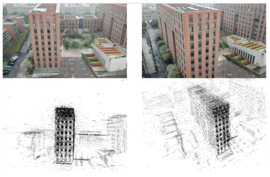
Figure 24.
Reconstruction results of the wall image set.
There are also some incorrectly reconstructed 3D lines in the model. The reasons for this can be summarized by the following two points. First, the matched line segment group was actually a mismatch. Second, camera pose errors caused some matched line segments to be incorrectly triangulated. Our method has reduced the error in the first point to a significantly lower level. As for the second point, some filtering methods for 3D space could be designed in the future to reduce these incorrectly reconstructed edges.
5. Conclusions
This paper presented a line-based 3D reconstruction method, Edge3D, and tested it on real-word image sets. Edge3D contains steps of matching line segments, edge recovery and triangulation, and bundle adjustment to effectively extract and reconstruct building edges in 3D space. It exploits information from a trifocal tensor, 3D reprojection errors, and line-based bundle adjustment to improve the line segment matching accuracy. It can reconstruct building models with a small number of images, benefiting from its ability to match line segments between images with small overlap. An endpoint-oriented bundle adjustment strategy is introduced to simplify and automate the non-linear optimization process. Testing on challenge real-world images, the presented algorithm achieves a matching precision of around 95%. It can retain richer features in a building model to avoid edge distortion and provide better visualization. Edge3D serves as a fundamental method for many IT applications, such as Digital Twin modeling [55] and IOT sensor embedding [56]. A limitation of the method exists in that the process of removing mismatching line segments is only operated on 2D images. Errors may also occur during the 3D reconstruction process. In the future, a promising direction is to reduce the mismatch cases in 3D space to compensate for existing limitations.
Author Contributions
Conceptualization, X.S.; data curation, J.C.; formal analysis, L.L.; investigation, J.C.; methodology, L.L.; resources, A.N.; software, L.L.; supervision, X.S.; validation, J.C. and A.N.; writing—original draft, L.L.; writing—review and editing, X.S. and A.N. All authors have read and agreed to the published version of the manuscript.
Funding
This work is funded by the Center for Balance Architecture, Zhejiang University and the National Natural Science Foundation of China (Grant No. 71971196).
Institutional Review Board Statement
Not applicable.
Informed Consent Statement
Not applicable.
Data Availability Statement
Not applicable.
Conflicts of Interest
The authors declare no conflict of interest.
References
- Dino, I.G.; Sari, A.E.; Iseri, O.K.; Akin, S.; Kalfaoglu, E.; Erdogan, B.; Kalkan, S.; Alatan, A.A. Image-based construction of building energy models using computer vision. Autom. Constr. 2020, 116, 103231. [Google Scholar] [CrossRef]
- Eicker, U.; Zirak, M.; Bartke, N.; Rodríguez, L.R.; Coors, V. New 3D model based urban energy simulation for climate protection concepts. Energy Build. 2018, 163, 79–91. [Google Scholar] [CrossRef]
- Kamel, E.; Memari, A.M. Review of BIM’s application in energy simulation: Tools, issues, and solutions. Autom. Constr. 2019, 97, 164–180. [Google Scholar] [CrossRef]
- Golparvar-Fard, M.; Ham, Y. Automated diagnostics and visualization of potential energy performance problems in existing buildings using energy performance augmented reality models. J. Comput. Civ. Eng. 2014, 28, 17–29. [Google Scholar] [CrossRef]
- Jiang, W.; Zhou, Y.; Ding, L.; Zhou, C.; Ning, X. UAV-based 3D reconstruction for hoist site mapping and layout planning in petrochemical construction. Autom. Constr. 2020, 113, 103137. [Google Scholar] [CrossRef]
- Hammad, A.W.A.; da Costa, B.B.F.; Soares, C.A.P.; Haddad, A.N. The use of unmanned aerial vehicles for dynamic site layout planning in large-scale construction projects. Buildings 2021, 11, 602. [Google Scholar] [CrossRef]
- Liu, C.-W.; Wu, T.-H.; Tsai, M.-H.; Kang, S.-C. Image-based semantic construction reconstruction. Autom. Constr. 2018, 90, 67–78. [Google Scholar] [CrossRef]
- Sánchez-Aparicio, L.J.; Masciotta, M.-G.; García-Alvarez, J.; Ramos, L.F.; Oliveira, D.V.; Martín-Jiménez, J.A.; González-Aguilera, D.; Monteiro, P. Web-GIS approach to preventive conservation of heritage buildings. Autom. Constr. 2020, 118, 103304. [Google Scholar] [CrossRef]
- Mora, R.; Sánchez-Aparicio, L.J.; Maté-González, M.; García-Álvarez, J.; Sánchez-Aparicio, M.; González-Aguilera, D. An historical building information modelling approach for the preventive conservation of historical constructions: Application to the Historical Library of Salamanca. Autom. Constr. 2021, 121, 103449. [Google Scholar] [CrossRef]
- Masciotta, M.; Sánchez-Aparicio, L.; Bishara, S.; Oliveira, D.; González-Aguilera, D.; García-Alvarez, J. Digitization of cultural heritage buildings for preventive conservation purposes. In Proceedings of the 12th International Conference on Structural Analysis of Historical Constructions (SAHC), Barcelona, Spain, 16–18 September 2020. [Google Scholar]
- Shang, Z.; Shen, Z. Real-time 3D reconstruction on construction site using visual SLAM and UAV. arXiv 2017, arXiv:1712.07122. [Google Scholar]
- Kaiser, T.; Clemen, C.; Maas, H.-G. Automatic co-registration of photogrammetric point clouds with digital building models. Autom. Constr. 2022, 134, 104098. [Google Scholar] [CrossRef]
- Wilson, L.; Rawlinson, A.; Frost, A.; Hepher, J. 3D digital documentation for disaster management in historic buildings: Applications following fire damage at the Mackintosh building, the Glasgow School of Art. J. Cult. Herit. 2018, 31, 24–32. [Google Scholar] [CrossRef]
- Dabous, A.S.; Feroz, S. Condition monitoring of bridges with non-contact testing technologies. Autom. Constr. 2020, 116, 103224. [Google Scholar] [CrossRef]
- Fathi, H.; Dai, F.; Lourakis, M. Automated as-built 3D reconstruction of civil infrastructure using computer vision: Achievements, opportunities, and challenges. Adv. Eng. Inform. 2015, 29, 149–161. [Google Scholar] [CrossRef]
- Scaioni, M.; Barazzetti, L.; Giussani, A.; Previtali, M.; Roncoroni, F.; Alba, M.I. Photogrammetric techniques for monitoring tunnel deformation. Earth Sci. Inform. 2014, 7, 83–95. [Google Scholar] [CrossRef]
- Marinello, F. Last generation instrument for agriculture multispectral data collection. Agric. Eng. Int. CIGR J. 2017, 19, 87–93. [Google Scholar]
- Tang, P.; Akinci, B.; Huber, D. Quantification of edge loss of laser scanned data at spatial discontinuities. Autom. Constr. 2009, 18, 1070–1083. [Google Scholar] [CrossRef]
- Inzerillo, L.; di Mino, G.; Roberts, R. Image-based 3D reconstruction using traditional and UAV datasets for analysis of road pavement distress. Autom. Constr. 2018, 96, 457–469. [Google Scholar] [CrossRef]
- Zhou, Z.; Gong, J.; Guo, M. Image-based 3D reconstruction for posthurricane residential building damage assessment. J. Comput. Civ. Eng. 2016, 30, 04015015. [Google Scholar] [CrossRef]
- Liénard, J.; Vogs, A.; Gatziolis, D.; Strigul, N. Embedded, real-time UAV control for improved, image-based 3D scene reconstruction. Measurement 2016, 81, 264–269. [Google Scholar] [CrossRef]
- Alidoost, F.; Arefi, H. An image-based technique for 3D building reconstruction using multi-view UAV images. Int. Arch. Photogramm. Remote Sens. Spat. Inf. Sci. 2015, 40, 43. [Google Scholar] [CrossRef]
- Yang, M.-D.; Chao, C.-F.; Huang, K.-S.; Lu, L.-Y.; Chen, Y.-P. Image-based 3D scene reconstruction and exploration in augmented reality. Autom. Constr. 2013, 33, 48–60. [Google Scholar] [CrossRef]
- Bleyer, M.; Rhemann, C.; Rother, C. Patchmatch stereo-stereo matching with slanted support windows. In Proceedings of the British Machine Vision Conference, Dundee, UK, 29 August–2 September 2011. [Google Scholar]
- Schönberger, J.L.; Zheng, E.; Frahm, J.-M.; Pollefeys, M. Pixelwise view selection for unstructured multi-view stereo. In Proceedings of the European Conference on Computer Vision, Amsterdam, The Netherlands, 8–16 October 2016; Springer: Cham, Switzerland, 2016. [Google Scholar]
- Golparvar-Fard, M.; Bohn, J.; Teizer, J.; Savarese, S.; Peña-Mora, F. Evaluation of image-based modeling and laser scanning accuracy for emerging automated performance monitoring techniques. Autom. Constr. 2011, 20, 1143–1155. [Google Scholar] [CrossRef]
- Bhatla, A.; Choe, S.Y.; Fierro, O.; Leite, F. Evaluation of accuracy of as-built 3D modeling from photos taken by handheld digital cameras. Autom. Constr. 2012, 28, 116–127. [Google Scholar] [CrossRef]
- Xu, Z.; Kang, R.; Lu, R. 3D reconstruction and measurement of surface defects in prefabricated elements using point clouds. J. Comput. Civ. Eng. 2020, 34, 04020033. [Google Scholar] [CrossRef]
- Zhou, Z.; Gong, J. Automated analysis of mobile LiDAR data for component-level damage assessment of building structures during large coastal storm events. Comput.-Aided Civ. Infrastruct. Eng. 2018, 33, 373–392. [Google Scholar] [CrossRef]
- Bartoli, A.; Sturm, P. Structure-from-motion using lines: Representation, triangulation, and bundle adjustment. Comput. Vis. Image Underst. 2005, 100, 416–441. [Google Scholar] [CrossRef]
- Micusik, B.; Wildenauer, H. Structure from motion with line segments under relaxed endpoint constraints. Int. J. Comput. Vis. 2017, 124, 65–79. [Google Scholar] [CrossRef]
- Fan, B.; Wu, F.; Hu, Z. Line matching leveraged by point correspondences. In Proceedings of the 2010 IEEE Computer Society Conference on Computer Vision and Pattern Recognition, San Francisco, CA, USA, 13–18 June 2010; IEEE: Piscataway, NJ, USA, 2010. [Google Scholar]
- Al-Shahri, M.; Yilmaz, A. Line matching in wide-baseline stereo: A top-down approach. IEEE Trans. Image Process. 2014, 23, 4199–4210. [Google Scholar]
- Schmid, C.; Zisserman, A. The geometry and matching of lines and curves over multiple views. Int. J. Comput. Vis. 2000, 40, 199–233. [Google Scholar] [CrossRef]
- Li, K.; Yao, J. Line segment matching and reconstruction via exploiting coplanar cues. ISPRS J. Photogramm. Remote Sens. 2017, 125, 33–49. [Google Scholar] [CrossRef]
- Wang, Z.; Wu, F.; Hu, Z. MSLD: A robust descriptor for line matching. Pattern Recognit. 2009, 42, 941–953. [Google Scholar] [CrossRef]
- Zhang, L.; Koch, R. An efficient and robust line segment matching approach based on LBD descriptor and pairwise geometric consistency. J. Vis. Commun. Image Represent. 2013, 24, 794–805. [Google Scholar] [CrossRef]
- Bay, H.; Ferraris, V.; van Gool, L. Wide-baseline stereo matching with line segments. In Proceedings of the 2005 IEEE Computer Society Conference on Computer Vision and Pattern Recognition (CVPR’05), San Diego, CA, USA, 20–25 June 2005; IEEE: Piscataway, NJ, USA, 2005. [Google Scholar]
- Wang, L.; Neumann, U.; You, S. Wide-baseline image matching using line signatures. In Proceedings of the 2009 IEEE 12th International Conference on Computer Vision, Kyoto, Japan, 29 September–2 October 2009; IEEE: Piscataway, NJ, USA, 2009. [Google Scholar]
- López, J.; Santos, R.; Fdez-Vidal, X.R.; Pardo, X.M. Two-view line matching algorithm based on context and appearance in low-textured images. Pattern Recognit. 2015, 48, 2164–2184. [Google Scholar] [CrossRef]
- Li, K.; Yao, J.; Lu, X.; Li, L.; Zhang, Z. Hierarchical line matching based on line–junction–line structure descriptor and local homography estimation. Neurocomputing 2016, 184, 207–220. [Google Scholar] [CrossRef]
- Kim, H.; Lee, S. Simultaneous line matching and epipolar geometry estimation based on the intersection context of coplanar line pairs. Pattern Recognit. Lett. 2012, 33, 1349–1363. [Google Scholar] [CrossRef]
- Fan, B.; Wu, F.; Hu, Z. Robust line matching through line–point invariants. Pattern Recognit. 2012, 45, 794–805. [Google Scholar] [CrossRef]
- Košecká, J.; Zhang, W. Video compass. In Proceedings of the European Conference on Computer Visio, Copenhagen, Denmark, 28–31 May 2002; Springer: Berlin/Heidelberg, Germany, 2002; pp. 476–490. [Google Scholar]
- Elqursh, A.; Elgammal, A. Line-based relative pose estimation. In Proceedings of the CVPR 2011, Colorado Springs, CO, USA, 20–25 June 2011; IEEE: Piscataway, NJ, USA, 2011. [Google Scholar]
- Zhang, L.; Koch, R. Structure and motion from line correspondences: Representation, projection, initialization and sparse bundle adjustment. J. Vis. Commun. Image Represent. 2014, 25, 904–915. [Google Scholar] [CrossRef]
- Ma, Z.; Liu, S. A review of 3D reconstruction techniques in civil engineering and their applications. Adv. Eng. Inform. 2018, 37, 163–174. [Google Scholar] [CrossRef]
- Li, K.; Yao, J.; Li, L.; Liu, Y. 3D line segment reconstruction in structured scenes via coplanar line segment clustering. In Proceedings of the Asian Conference on Computer Vision, Taipei, Taiwan, 20–24 November 2016; Springer: Cham, Switzerland, 2016; pp. 46–61. [Google Scholar]
- Jain, A.; Kurz, C.; Thormahlen, T.; Seidel, H.-P. Exploiting global connectivity constraints for reconstruction of 3D line segments from images. In Proceedings of the 2010 IEEE Computer Society Conference on Computer Vision and Pattern Recognition, San Francisco, CA, USA, 13–18 June 2010; IEEE: Piscataway, NJ, USA, 2010. [Google Scholar]
- Hofer, M.; Maurer, M.; Bischof, H. Efficient 3D scene abstraction using line segments. Comput. Vis. Image Underst. 2017, 157, 167–178. [Google Scholar] [CrossRef]
- Sun, Y.; Zhao, L.; Huang, S.; Yan, L.; Dissanayake, G. Line matching based on planar homography for stereo aerial images. ISPRS J. Photogramm. Remote Sens. 2015, 104, 1–17. [Google Scholar] [CrossRef]
- Wei, D.; Zhang, Y.; Liu, X.; Li, C.; Li, Z. Robust line segment matching across views via ranking the line-point graph. ISPRS J. Photogramm. Remote Sens. 2021, 171, 49–62. [Google Scholar] [CrossRef]
- Schonberger, L.J.; Frahm, J.-M. Structure-from-motion revisited. In Proceedings of the IEEE Conference on Computer Vision and Pattern Recognition, Las Vegas, NV, USA, 27–30 June 2016. [Google Scholar]
- Wu, C. VisualSFM: A Visual Structure from Motion System. 2011. Available online: http://www.cs.washington.edu/homes/ccwu/vsfm (accessed on 1 August 2022).
- Minos-Stensrud, M.; Haakstad, O.H.; Sakseid, O.; Westby, B.; Alcocer, A. Towards automated 3D reconstruction in SME factories and digital twin model generation. In Proceedings of the 2018 18th International Conference on Control, Automation and Systems (ICCAS), PyeongChang, Korea, 17–20 October 2018; IEEE: Piscataway, NJ, USA, 2018. [Google Scholar]
- Massaro, A.; Manfredonia, I.; Galiano, A.; Contuzzi, N. Inline image vision technique for tires industry 4.0: Quality and defect monitoring in tires assembly. In Proceedings of the 2019 II Workshop on Metrology for Industry 4.0 and IoT (MetroInd4.0&IoT), Naples, Italy, 4–6 June 2019; IEEE: Piscataway, NJ, USA, 2019. [Google Scholar]
Publisher’s Note: MDPI stays neutral with regard to jurisdictional claims in published maps and institutional affiliations. |
© 2022 by the authors. Licensee MDPI, Basel, Switzerland. This article is an open access article distributed under the terms and conditions of the Creative Commons Attribution (CC BY) license (https://creativecommons.org/licenses/by/4.0/).