1. Introduction
To achieve a high-quality building, many aspects must be considered. The relative importance of the different aspects has changed over time, and in recent years the environmental footprint of a building has become increasingly relevant, due to the urgent need to reduce global warming. The layer of insulation in a building envelope has two purposes, ensuring a comfortable indoor climate, and reducing heat loss and thus saving both energy and money. The manufacturing and transportation of insulation materials are both energy-demanding processes, and the reduction in heat loss per mm of insulation decreases with the increase in the insulation thickness. Therefore, there must be an optimum CO
2-oriented insulation thickness. The focus of this research is on the insulation of wall constructions. In a Norwegian study, the operational emissions of CO
2-eq have been identified as being much more sensitive to the insulation thickness in walls than in roofs or floors in a conventionally shaped house [
1].
Most of the building regulations stipulate a maximum U-value for each part of a building, which must be met along with the demands on the overall energy consumption of the building. In the current Greenlandic building regulations from 2006 [
2], the dimensioning energy demand of a building distinguishes between the areas north and south of the Arctic Circle, but, otherwise, the regulations do not account for the climatic and energy production conditions of each town and settlement. From a comfort and health point of view, this makes sense. However, the energy sources may differ considerably, from hydropower to oil, so that the same heat loss in two different locations can have different environmental impacts, based on the emitted Greenhouse Gases (GHG). An open-source Excel tool has been developed to simplify the process of defining the optimal insulation thickness based on multiple parameters, including insulation material, location and heating method. The tool is named “ITO”, which stands for “Insulation Thickness Optimizer”.
Insulation is a never-ending hot topic, including material development and comparison, optimal thicknesses, correct placement in the construction and emerging issues such as mold and rot. The volume of literature within this field is immense. However, defining the optimal insulation thickness for a location of interest can be completed in many ways, as there are many available indicators and parameters that can be used in this analysis. In particular, an economic benchmark is popular, defining the payback period, after which the investment in the insulation becomes beneficial compared to the cost savings due to the reduction in heat loss. One of the studies working from this perspective was that of Ozel [
3], who showed that the thermal conductivity (R) of a construction without insulation leads to an increased optimal insulation thickness and energy savings, while the payback period of the insulation decreases. The location of the study was Turkey, which is reflected in the recommended optimal insulation thickness of only 2.0–8.2 cm, depending on the scenario. Another study with a similar approach was Iranian and concluded that a maximum of 4 cm is the optimal insulation thickness (Rosti et al., 2020) [
4]. In [
4], the authors attributed the outcome to cheap electricity prices and claimed that the energy policies or pricing mechanisms should be adjusted to encourage the proper insulation of buildings, so as to ensure reduced heat loss and GHG emissions.
The new tool, ITO, introduced in this paper uses CO
2 emission as a benchmark for an optimal insulation thickness. This approach has been used in other studies. For example, the three Turkish papers [
5,
6,
7] all used a Life Cycle Assessment (LCA) method to analyze a fictive brick-wall case. They all reached different conclusions on the optimal insulation thicknesses for the individual cases, which makes it difficult to compare the results. However, these papers demonstrated an obvious interest in the dynamics between the insulation thicknesses, energy savings, emission reduction and, in many cases, economic aspects. This indicates the value of a simple tool, such as ITO, which can automatically make such calculations. In its present form, ITO does not consider Life Cycle Costs (LCC) because the values of the materials and energy resources change continuously, but it will eventually be possible to replace all of the environmental inputs with economic inputs to achieve an output based on the economic considerations instead of the climate impact. A recent study from 2021 by Dylewski et al. [
8] considered energy consumption for both the heating and cooling in the search for an optimal insulation thickness. The benchmark was a metacriterion including both the economic and ecological aspects with equally weighted importance. In addition, Janusz Adamczyk et al. [
9], and Spanodimitriou et al. [
10] considered both the economic and ecological perspectives, however Adamczyk et al. used HDD and Spanodimitriou et al. performed simulations and included considerations regarding the wall orientations. The latter study concluded that the best results were achieved for an east–west orientation of the building, compared to a north–south oriented building. This decision could save up to 13.6% energy. The Greek paper (Axaopoulos et al. 2019) considered the wall orientation as a variable parameter when defining the optimal insulation thickness [
11]. Dynamic simulations were performed of a system with different orientations. The paper considered four different climate zones, with varying Heating Degree Days (HDD) and U-value regulations, and concluded that the south-facing walls should have less insulation, while the north-facing walls should have more insulation. A study by Ounis, S. et al. [
12] changed the focus from the specific insulation material and investigated the needed U-value in different countries instead. A full map of Europe, excluding Greenland, was presented and the recommended U-value for Denmark was concluded to be 0.12 W/m
2 K, based on HDD
20 °C and CDD
24 °C.
Regardless of whether the focus is on the LCC or LCA, the climate plays a role, and as the service life of buildings is long, climate change may be expected to affect the results. This is something that none of the presented papers considers when defining the optimal insulation thickness. The rising temperatures will lead to lower HDD and consequently, the heat loss of the construction will be reduced. This might result in a decrease in the optimal insulation, regardless of the focus. ITO can evaluate three climate scenarios, as well as constant HDD. The user can easily adjust the temperature change for each scenario, but the tool has three initial settings, based on the information from the Intergovernmental Panel on Climate Change (IPCC), which is currently developing the sixth report on climate change, investigating the extent of global warming [
13]. It has already been concluded that climate change is experienced in every region of the globe.
ITO is intended to be a simple tool that a building designer can use to determine the optimal insulation thickness in a given situation. A thorough determination of the optimal insulation thickness is very demanding, and, for most buildings, it is unlikely to be performed, especially in single-family houses in Greenland. With ITO, the issue can more easily be considered and contribute to more sustainable decision-making, as it delivers an indication of the optimal insulation thickness.
The present paper describes the development of ITO. In
Section 2, Method, the fundamental equations, assumptions and considerations are presented. The section ends with a presentation of the input and output parameters of the tool, details about the considered insulation materials and a definition of a wall construction, which is used as a case during the article. In
Section 3, Results, some of the outputs produced by ITO are presented for five chosen destinations. The section includes both the simple results considering the insulation alone and the results for insulation implemented in the case of a wall construction. The results are analyzed in
Section 4, Analysis, which consists of three parts; a sensitivity analysis testing the robustness of the tool; an investigation of the impact of emissions from elements, which are defined to be beyond the system boundary; and finally, an analysis of the results when changing the definition of “optimal insulation thickness” to be less strict. Some of the content from the previous sections is discussed in
Section 5, Discussion, followed by a conclusion, which is the final part of this article.
2. Method
The tool was developed in Microsoft Excel, together with user-friendly guidelines. It is intended to be used for decision-making both by the building industry and by individual building owners. The tool is based on standard methodologies and equations for thermal matters, and LCA, and uses data from the literature and available databases.
2.1. System
When trying to define the optimal insulation thickness, dopt, it is necessary to define the success criteria. The first aspect of this is deciding on which parameter the balance should depend. There are three obvious possibilities, energy (kWh), greenhouse gas emissions (kg CO2-eq) and monetary cost. As ITO is intended to promote better decisions in terms of sustainability, the benchmark parameter was chosen to be GHG emissions. This parameter takes into account the fact that different energy sources have different climatic impacts.
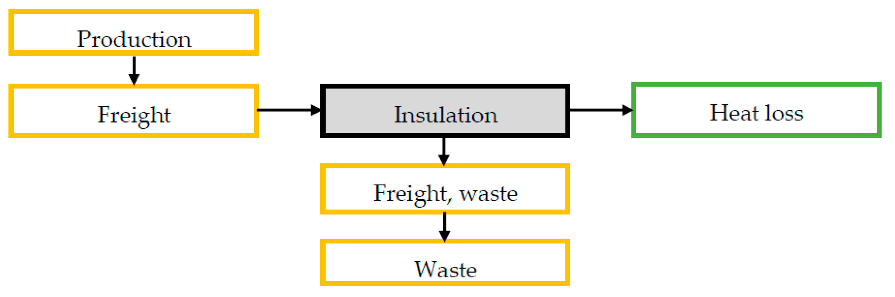
Figure 1 illustrates the product system for the insulation. The yellow boxes are processes that contribute to the emissions arising from the insulating material (
Ematerial (kg CO
2-eq/m
3)), while the green box denotes the emissions related to the resulting heat losses,
. Equation (1) clarifies the relation between the yellow boxes and quantifies the total GHG emissions for 1 m
3 insulation,
Ematerial. The indices refer to the yellow boxes in
Figure 1:
In theory, the best insulation thickness is found when the reduction in the greenhouse gas emissions (GHG), achieved by the insulation, equals the emitted GHG caused by the production and handling of the insulation. This can be expressed very simply by
, where
is the emission difference relating to the reduced heat loss through the wall caused by the insulation. In practice, however, this criterion is challenged because the reduced heat loss cannot be calculated without defining a starting point, which would require a definition of the additional construction layers of the wall. In the tool, this will be an option but not a necessity. Furthermore, there might be situations where this equation is never fulfilled with a realistic thickness. Therefore,
dopt is defined to be the thickness,
d, with minimum emissions,
E, which is described as
E(dopt) in Equation (2):
The tool calculates the emissions for each stage for 1 m3 insulation material and cumulates them. The sum of Eheat and Ematerial for 1 m2 wall is then calculated in a list with increasing insulation thicknesses, starting from 5 mm. In this list, the minimum level of CO2-eq emissions can be identified along with the corresponding thickness. Because of this approach, all of the equations regarding emissions are given for 1 m3 of material.
2.2. Life Cycle Stages
To calculate the total material emissions (
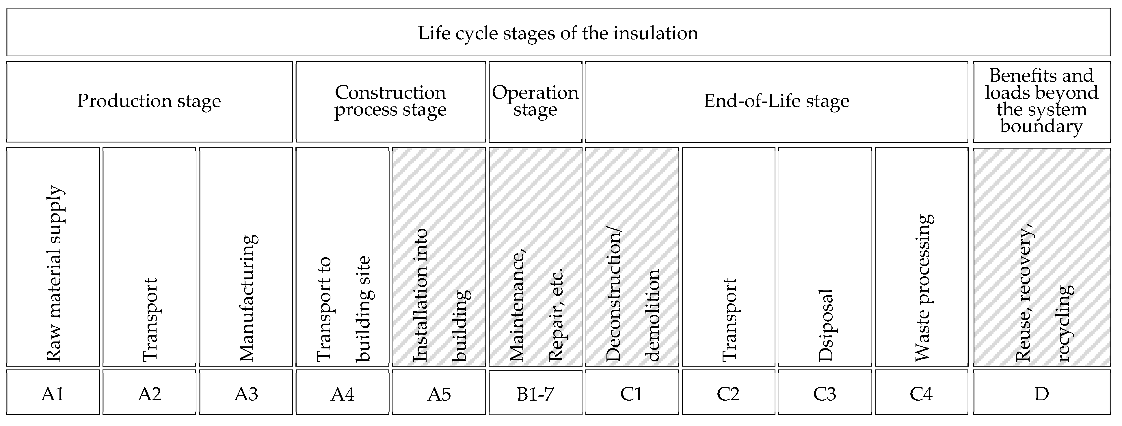
Ematerial) it is necessary to consider all of the aspects of its life cycle. There are multiple phases to LCA.
Figure 2 illustrates the many phases, which elaborate on the yellow boxes in
Figure 1. Four of the boxes are hatched to show that they are not considered by the tool. A5, “installation into buildings” and C1, “deconstruction and demolition” are disregarded, because their contribution to the system is small and quantifying them would involve too many assumptions without changing the outcome significantly. The operation stage of the insulation, B1-7, is not included as it is expected that the material will last as long as the building itself, meaning that no repairs or replacement of the insulation material will be necessary. The maintenance of the entire wall is assumed to be independent of the insulation thickness. Furthermore, the operation of the insulation does not require fuel or other resources, which B1-7 also accounts for. The last stage, D “Benefits and loads beyond the system boundary,” is usually given in the product datasheet, but the impacts depend on the current state of the art, which is why including it in such a long-time perspective could be misleading. The value of D can both be positive and negative. The negative values are possible because D accounts for any heat gained from incineration, or an amount of insulation produced with less raw materials due to recycling. Furthermore, Stage D depends on the perspective and method of the product datasheet, which is not always transparent, and is thus difficult to compare. In some of the datasheets, the saved energy from Stage D exceeds the emissions from the other phases, indicating that the more material consumption the greater the sustainability, which can never be the case. Due to the uncertainties of these data, D is not considered in the tool.
2.2.1. Production and Operation Stage
The emissions from the production stage (
EA1-3) are given in the product datasheets for each material. For the pre-coded materials, the free software “LCAbyg 5” [
15] is used to find these data, and the ITO shows the exact sources. The sources used in the ITO give A1-3 in kg CO
2-eq/m
3, but it may vary for the different datasheets. During production and transportation, there will be a waste fraction (
Wmaterial). How much is uncertain, but this value is usually between 2 and 10% at the factory. As the material may have to be transported a long way from the factory to the building site, it is recommended to set the value at the high end of this span or even slightly above. Equation (3) calculates the emissions caused by producing 1 m
3 insulation,
Eprod:
2.2.2. Construction Stage
The emissions caused by A4 “Transport to the building site”, are based on the production country given in the product datasheet and the location of the building site. It is assumed that there are three transportation methods: truck; boat and plane. It is unusual to transport building materials by plane, but the option is implemented for certain cases. All of the materials listed in the tool are produced in Europe. It is assumed that all of the materials are produced somewhere in the middle of the selected country. If the building site is placed in Copenhagen, it is assumed that the materials are taken by truck directly from the factory. For the Greenlandic destinations, it is assumed that the insulation is transported by truck to an industrialized harbor in the same country and then shipped to the specific harbor of the destination. Royal Arctic Line has an exclusive concession with the Greenlandic government, covering all of the sea cargo in Greenland, both internally and externally [
16]. According to the Royal Arctic Line webpage, all of the transportation out of Greenland passes through Reykjavik and ends in Aalborg harbor [
16]. Based on this, the distances, D, in km for each mode of transportation are estimated by using the measurement tool in Google Maps [
17]. The transportation emissions are from Ecoinvent 3, consequential unit [
18] processed in SimaPro version 9.2.0.2 [
19] and the method used is ReCiPe 2016 Midpoint (H) [
20]. The chosen process for boat transportation emits
Eboat = 0.00959 kg CO
2/tkm, the truck emits
Etruck = 0.167 kg CO
2/tkm and the plane emits
Eplane = 0.436 kg CO
2/tkm. Equation (4) assumes that half of the wasted material,
Wmaterial, will be transported all of the way to the building site. This is a rough estimation that some of the waste will occur at the building site. ρ is the density of the insulation in kg/m
3.
2.2.3. End of Life Stage and Benefits and Loads beyond the System Boundary
The End-of-Life (EoL), for a material has multiple options, such as landfill, incineration, recycling and reuse. Currently, the options for reuse and recycling are very limited in Greenland, which is why most of the waste materials end up in landfills. If the location can facilitate incineration, it will most likely be the preferred solution. It is planned that the incinerators in Nuuk and Sisimiut should be modernized by 2023, making it possible in these two locations to incinerate the content of the dumps and the waste of all the other settlements and cities [
21]. To reuse or recycle the waste, it is necessary to transport the waste materials to other countries, e.g., Denmark or Germany. Whether or not this emits less GHG is case dependent, but generally, recycling or reuse through other countries is unlikely. Based on this information, it was decided to make default settings for incineration and landfill for each location, while recycling is left as a possible manually selected option for those cases in which detailed information is available.
EoL, covering C2-C4 in
Figure 2, is often given in the product datasheet, but the transportation, C2, is highly dependent on the location of the building site and must be evaluated based on the Greenlandic conditions. In ITO, it is assumed that all of the waste is transported by boat to either Nuuk or Sisimiut and incinerated. ITO assumes that it is moved to the nearest of the two, however that might be different in practice. If the material is landfilled, it is assumed to be taken by truck across the city. The equation for
Efreight,waste is the same as for
Efreight, presented in Equation (4). The equation for
Ewaste is presented in Equation (5), where
Wmaterial is the unitless waste factor and E
C3 and E
C4 are the EoL-stages presented in
Figure 1, given in kg CO
2-eq/m
3:
2.3. Heat Loss and Emissions
The tool considers heat loss in two scenarios: an individual layer of insulation material, Scen
ins, and a full wall construction, Scen
wall. The first mentioned is simple to apply, as it does not require any information beyond the system presented in
Figure 2. The result of this method is unreliable from a practical perspective but can be used to identify the correlations between the choices of inputs. Scen
wall demands more initial knowledge about the whole wall construction, which will provide more accurate definitions of the optimal insulation thickness and the correlating GHG emissions. Working with the second scenario and considering the whole wall, it is important to be aware that it does not consider the emissions related to the additional construction materials used to build the wall.
The heat loss through a wall can be calculated with varying precision, ranging from complicated simulations to simple estimations. To facilitate the regular practitioner, the priority, in this case, was to keep the tool simple and quick to use, with few demands on software. Therefore, the heat loss calculations are based on Heating Degree Days (HDD), a method that can be performed in Excel or any other spreadsheet. This compromises the accuracy of the results, however, it will indicate an optimization that will not be prioritized if the process is too demanding of time and money.
Eheat is an expression for the emissions related to the heat loss of the insulation or wall, depending on the approach. It is calculated by Equation (6), where
Efactor is the emission factor, quantifying the amount of kg CO
2-eq per kWh heat:
The heat loss caused by transmission (
Q) depends on the heat conductivity,
λ (W/mK), and on the insulating material and its thickness (
d (m)). As a simplification, only thermal conductivity is considered, and only a simple wall. The doors, windows, thermal bridges, etc. are disregarded. The climate plays an active role, as shown in Equation (7), where
HDD is the Heating Degree Days (K days/year))for the location,
(U (W/m
2 K)) is the heat transmission coefficient of the insulation material and
ESL is the Estimated Service Life (year).
ESL is an independent variable, which can be set from 10 to 110 years, while 60 years is the most common value used for dimensioning. Equation (7) calculates
Q for 1 m
2 wall (kWh/m
2):
Wdist is the heat loss caused by the distribution of heat. This is usually 2–10% for district heating [
22], and in the low end for local heating with e.g., oil. By default, this tool provides two options for heating, but in specific cases with in-depth knowledge about the heating, the factors can be changed accordingly. The two default options are local heating with oil and district heating (dh). The emission factors relating to the heating source (
Efactor) are individual for the district heating at each location. Usually, district heating in Greenland consists of incineration, hydropower and the burning of oil.
Table 1 shows the emission factors for the default locations in the tool. If the building is heated solely by oil, the emission factor is defined to be 0.335 kg CO
2-eq/kWh. Not all of the towns and settlements in Greenland have access to district heating, but the default towns in ITO do have.
The default locations in the tool represent a variety of cities in Greenland, where Nuuk is the absolute largest with 19,000 inhabitants [
24] and Qaanaaq is the smallest with 619 residents [
25]. The second largest is Sisimiut, with more than 6000 inhabitants [
26]. There are gaps in the list of the cities, because of missing information about
HDD and
Efactors. With sufficient information, the tool can be edited to cover any desired location. The heat loss through the wall is calculated by using
HDD, instead of the usual dimensional indoor and outdoor temperatures. Heating degree days,
HDD, is a measure for the difference of 1 K between the indoor mean temperature of 17 °C and the external average temperature over 24 h [
27]. In Denmark, the heating season spans from May to October, and the months are considered individually; the average sum of
HDD in the heating season over 5 years results in 2500 degree days, which is implemented in the tool [
27]. In Greenland, it is common to heat residential buildings all of the year, which is why an average of the latest 5 years of
HDD is used for the individual locations. The heating degree days are provided by Grønlands Statistikbank [
28]. For Uummannaq, the source did not include
HDD for the last 5 years. Thus, the implemented value is for 2020 alone. The degree days for all of the locations are given in
Table 1.
The total emissions of 1 m
2 insulation (
Ed) with a given thickness of insulation (
d) can be calculated by Equation (8):
2.4. Climate Change
Climate change will lead to extensive changes all over the world, but especially in the Arctic, where the temperature is rising more rapidly than elsewhere [
29]. As climate change is a future circumstance, the exact development is unknown. Thus, the Intergovernmental Panel on Climate Change (IPCC) has developed different scenarios called the Representative Concentration Pathways (RCP). The original four RCPs are RCP2.6, RCP4.5, RCP6 and RCP8.5. The numbers describe the radiative forcing values range in 2100 with the unit W/m
2. For each RCP there are multiple predictions about how the individual scenario will affect the temperatures in the future, and the low RCPs lead to lower temperature differences.
The tool, ITO, considers three climate scenarios for a period of up to 110 years besides a constant scenario. The first and most “conservative” scenario predicts a change of 0.2 °C/10 years. This is based on the data showing that the Earth’s surface temperature has generally risen by 0.18 °C/10 years since 1981 [
29]. This development is between RCP1.9 and RCP2.6, of which the latter is likely to keep the temperature rise below 1.5 °C, and thus fulfil the Paris Agreement. The second scenario predicts 0.4 °C/10 years based on the median-predicted temperature rise for RPC8.5, which is a scenario with high GHG emissions. This scenario is called “moderate”, however, it is currently at the high end of the expectations of experts. The last and most “extreme” scenario is 2.7 °C/10 years. This is based on IPCC claiming that the surface temperatures during winter in the central Arctic were 6 °C higher in 2016 and 2018 compared to the average of 1981–2010 [
30]. The 2.7 °C/10 years is calculated as a 6 °C temperature increase over 22 years (the middle year of each interval 1995 and 2017). The default scenarios are set to investigate how climate change might reduce the need for insulation, but they can be adjusted as desired in the tool.
The climate development is simplified by identifying the change in the heating degree days (
HDDchange) for every 10th year caused by the temperature change (
Tchange). Equation (9) shows the calculation completed for every period of 10 years:
The change is implemented by calculating the heating degree days for every period. Based on the information about the ESL of the building, the tool cumulates the total HDD for the lifetime of the building.
2.5. Inputs and Outputs
The developed tool, ITO, can be found in the repository [
31]. In the present paper, the main features are presented. ITO requires a list of inputs, of which some are very straightforward, while others are important but uncertain information. The tool was developed to make it possible to use it with limited information, or if desired, with a higher level of detail or accuracy, by user-defining the inputs. As stated in
Section 2.3., the tool evaluates two setups: the insulation as a stand-alone scenario, Scen
ins; and a full wall, Scen
wall, which considers the secondary construction materials. Due to the analysis described later in
Section 4.2., it was decided to add “Scen
slab”, a scenario accounting for the emissions related to the slabs, roof and foundation. The reason is that thicker walls demand larger slabs. The Scen
slab can be combined with both Scen
ins and Scen
wall.
Table 2 lists the necessary information needed for each setup.
The tool considers two heating sources, and the system automatically presents the results for both of the options, so it is not an input parameter.
Table 3 shows all of the materials that were considered and their properties. It is assumed that the environmental impact of landfilling will be 0.01364 kg CO
2-eq per kg material [
32] and identical for all of the materials.
To present and analyze the functionality and results of the full wall, Scen
wall, it is necessary to predefine a wall. It is very common to build with ventilated walls in Greenland. To make sure that the wall is representative of the construction sector, a composition assessed in a previous study will be used. The wall was first presented in [
33] and is a heavy construction, as described in
Table 4. The wall contains a ventilated cavity, and according to the Danish Standard DS 418 [
34], the R-value of the cavity and the following external layers can be replaced by the internal heat transmission factor, R
si, for the same construction. In this case, the R
si is 0.130 m
2 K/W. The external standard for R
se is 0.040 m
2 K/W.
The outputs of the tool consist of both intermediate results, covering the balance of emissions for 1 m3 of insulation and a final recommendation of an optimal thickness of insulation for both oil and district heating. The latter is supported by graphs.
3. Results
Table 5 shows the results produced by ITO for five of the available ten cities and all of the eight materials. The five cities are Copenhagen, Nuuk, Sisimiut, Aasiaat and Qaanaaq, ordered with the most southern location first and the most northern location last. This also means that the number of heating degree days increases from Copenhagen to Qaanaaq. The parentheses after the location name shows the emission factor for the district heating at that location. Today, the Greenlandic requirements for the maximum U-values are 0.30 W/m
2 K and 0.20 W/m
2 K for heavy and light wall constructions, respectively [
2]. These demands can usually be met with 200 mm of insulation. However, it is expected that the new regulations will be implemented soon, and the requirements are expected to be tightened to 0.15 W/m
2 K for all of the wall types [
35]. This can typically be fulfilled with approximately 250 mm of insulation. E
d25 represents the total amount of emissions for 250 mm of insulation for comparison with the optimal insulation thickness. The results in
Table 5 are for Scen
ins, which excludes the additional wall structure and only considers the insulation.
The results in
Table 5 show that the cities with low emission factors, such as Nuuk, require less insulation. The maximum thickness for minimum GHG emissions is 1.72 m, which is extremely high (Wooden fibers in Aasiaat). This is also the combination with the most emissions at E
d25. The thinnest optimal insulation thickness is found for Cellulose fiber batts in Nuuk, and the least emissions to achieve
dopt is found for Wooden fiber in Nuuk. This combination also had the lowest
Ed25. Most of the scenarios lead to thicker insulation layers than are usually needed to fulfil the current and future building regulations. Regardless of the building location, choosing Cellular glass, Cellulose fiber batts or EPS 22.7 kg/m
3 lead to the thinnest layers of insulation. The Loose cellulose fiber and Wooden fiber lead to the thickest, optimal insulation thicknesses. For all of the locations, except Copenhagen, the Wooden fiber emits less CO
2 to obtain the optimal insulation thickness than the Cellulose fiber. It is worth noting that the optimal insulation thickness is greater for Copenhagen than for Nuuk, which indicates the importance of the emissions related to heating. Cellulose fiber batt is the best overall regarding
dopt but also the worst overall regarding
Eopt. The opposite counts for Wooden fiber, which is the best overall regarding
Eopt and almost the worst regarding
dopt, only exceeded by Loose cellulose fiber.
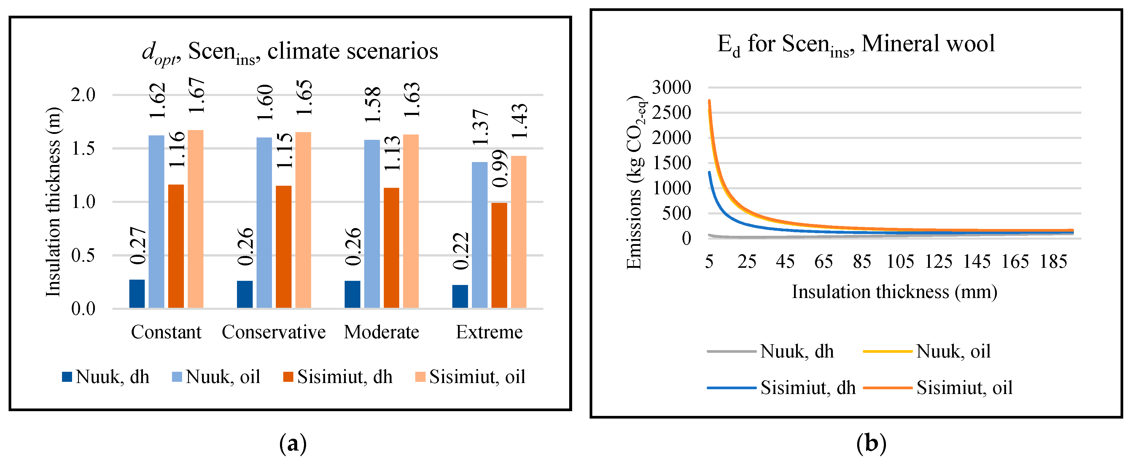
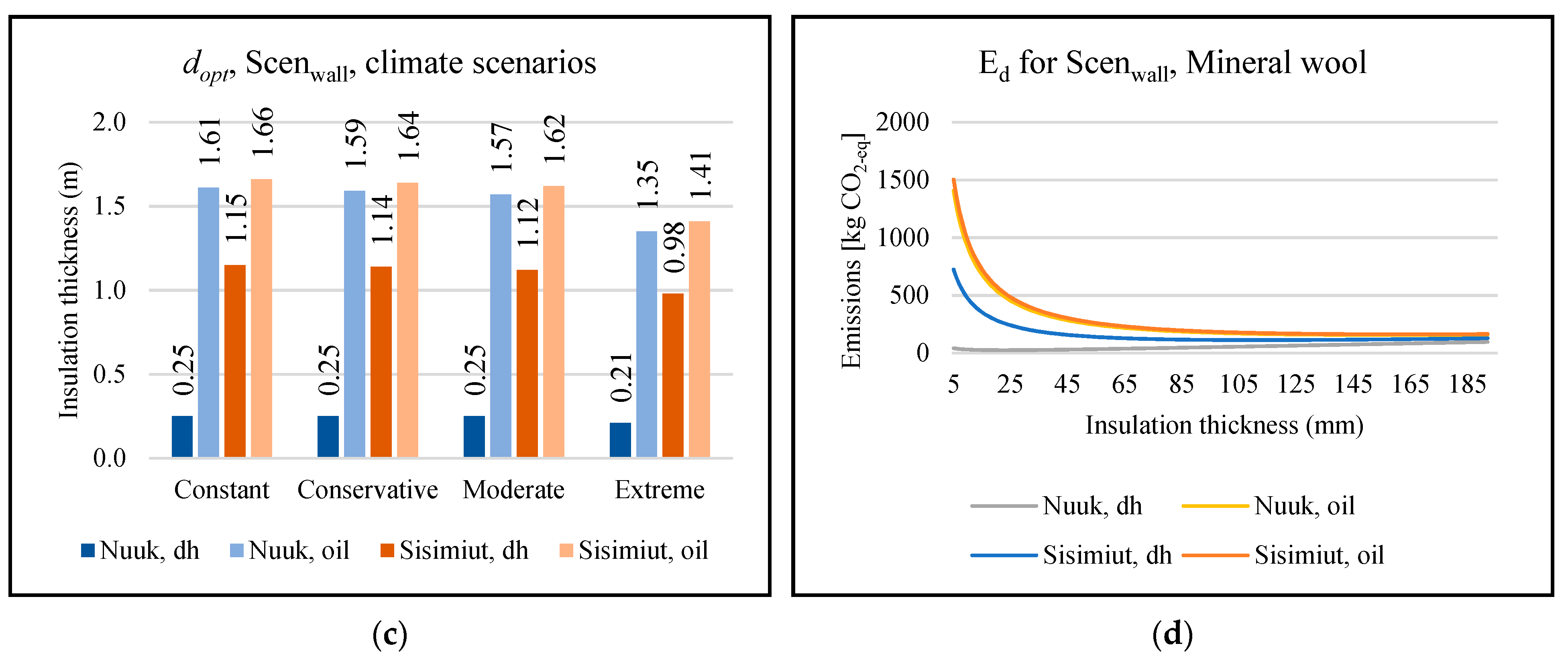
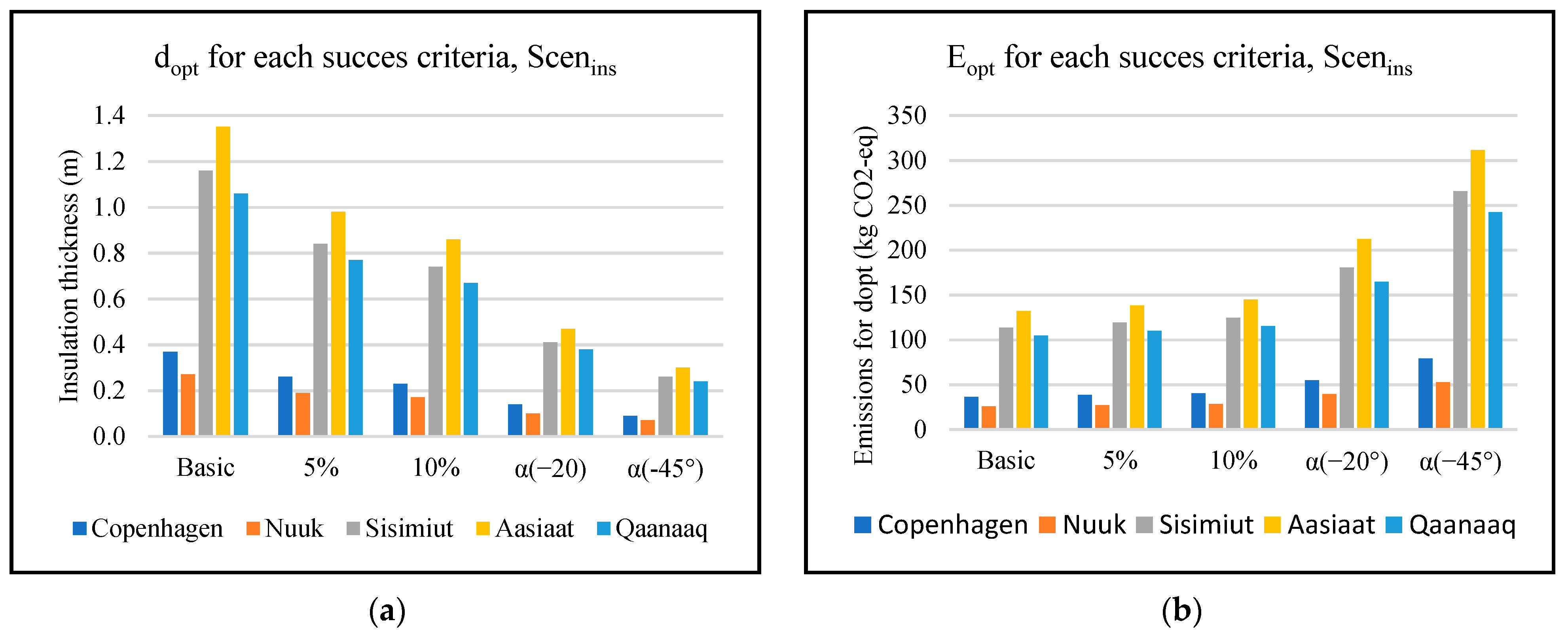
The main purpose of the four graphs in
Figure 3 is to compare the climate scenarios and the scenario Scen
ins with Scen
wall. A comparison of (a) and (c) shows that the additional layers of the wall have a very limited impact on the optimal insulation thickness, less than 3 mm thickness difference, in these cases. This is explained by (b) and (d), showing that the flow of the correlation between the emissions and the insulation thickness barely changes. This means that the optimum does not move either. However, the y-axes are very different, resulting in much lower total emissions at
dopt in cases with thin insulation layers. The thicker the
dopt, the less change in the emissions for the two scenarios. If, however, the chosen thickness is thinner than the
dopt, the additional layers will be significant in identifying the total emissions of CO
2. All of the graphs in
Figure 3 show that the buildings heated by oil generally require thicker insulation than those heated with district heating. The energy mix in Sisimiut emits more GHG than the mix in Nuuk, and the city has a higher level of heating degree days during a year. Thus, thicker insulation is necessary for the buildings in Sisimiut than in Nuuk to achieve a minimum of GHG. Finally,
Figure 3 shows that global warming, considered with the three climate scenarios, causes minimal changes in the optimal insulation thickness when the
Efactor is small e.g., when district heating consisting mainly of hydropower is used. The figure also shows that the tool demands very thick layers of insulation when the goal is to fulfil Equation (2). In the next section, it will be discussed how the criteria can be modified. In the following sections, only a constant climate will be considered.
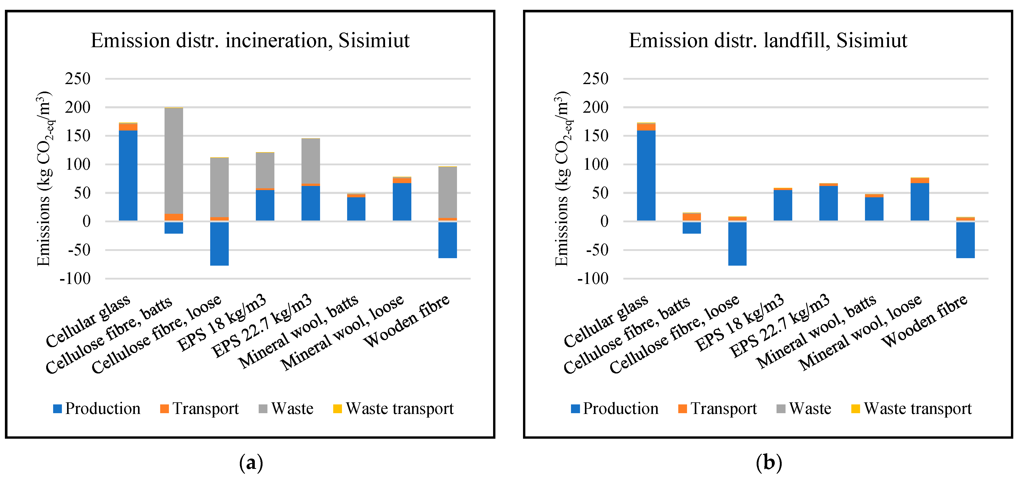
Figure 4 shows that transportation generally is of less importance in the bigger picture. Based on the inputs in the emission factors for transportation presented in
Section 2.2. that is because of the transportation method. If planes were chosen instead of trucks and boats, then the distance would have a bigger impact. The graphs also indicate that the impact of transportation has a bigger share of the total emissions when the waste ends as landfill, because it has fewer related emissions than incineration.
From the graphs, it can be seen that the Cellulose fiber batts and Cellular glass are the costliest to produce in terms of CO2-eq when incinerated. When using landfills, the Cellular glass performs worst, while the production of the Cellulose fiber and Wooden fiber reduces the CO2 by binding it to the material. ITO neglects the heat recovery possibilities of incineration.
5. Discussion
The tool has some obvious limitations. First, it does not consider possible moisture issues in the wall construction. The reason is partly that it demands information about each material included in the wall composition, and partly that it was not the purpose of the tool. If one wants to use the tool for that purpose as well, it is an option to implement a Glaser scheme or similar in a spreadsheet that uses the information from the pre-coded data. In addition, the tool represents oil and district heating, while many households in Greenland use only or partly electric heating. This is not included in the standard tool because of limited sources to indicate the use of energy.
In
Table 1, the
Efactor for Uummannaq stands out with the factor of 2 g CO
2-eq/kWh, while the second-lowest factor is for Nuuk (9 g CO
2-eq/kWh) and the third-lowest is for Copenhagen (49.9 g CO
2-eq/kWh). The reason for such low energy factors in Greenland is claimed to be hydropower, but Uummannaq has questionable low emission factors because hydropower usually emits 4 to 14 g CO
2-eq/kWh. It has even been estimated to be up to 150 g CO
2-eq/kWh for reservoir hydropower, which is usually used in Greenland [
36]. The source for the emission factors is Nukissiorfiit, which is the company that provides energy and water to most of Greenland and is thus the best informed on this topic. The question is whether it is important enough for them to carry out research and investigations, quantifying the actual
Efactor for each location in Greenland. The point of this discussion is not to question the honesty of Nukissiorfiit and the intentions of informing others about the sustainability of the energy production, but to create awareness of the difficulties and costs in quantifying such information, especially when fewer than 1000 people are affected. In general, more information and data on energy in Greenland would be valuable for future research.
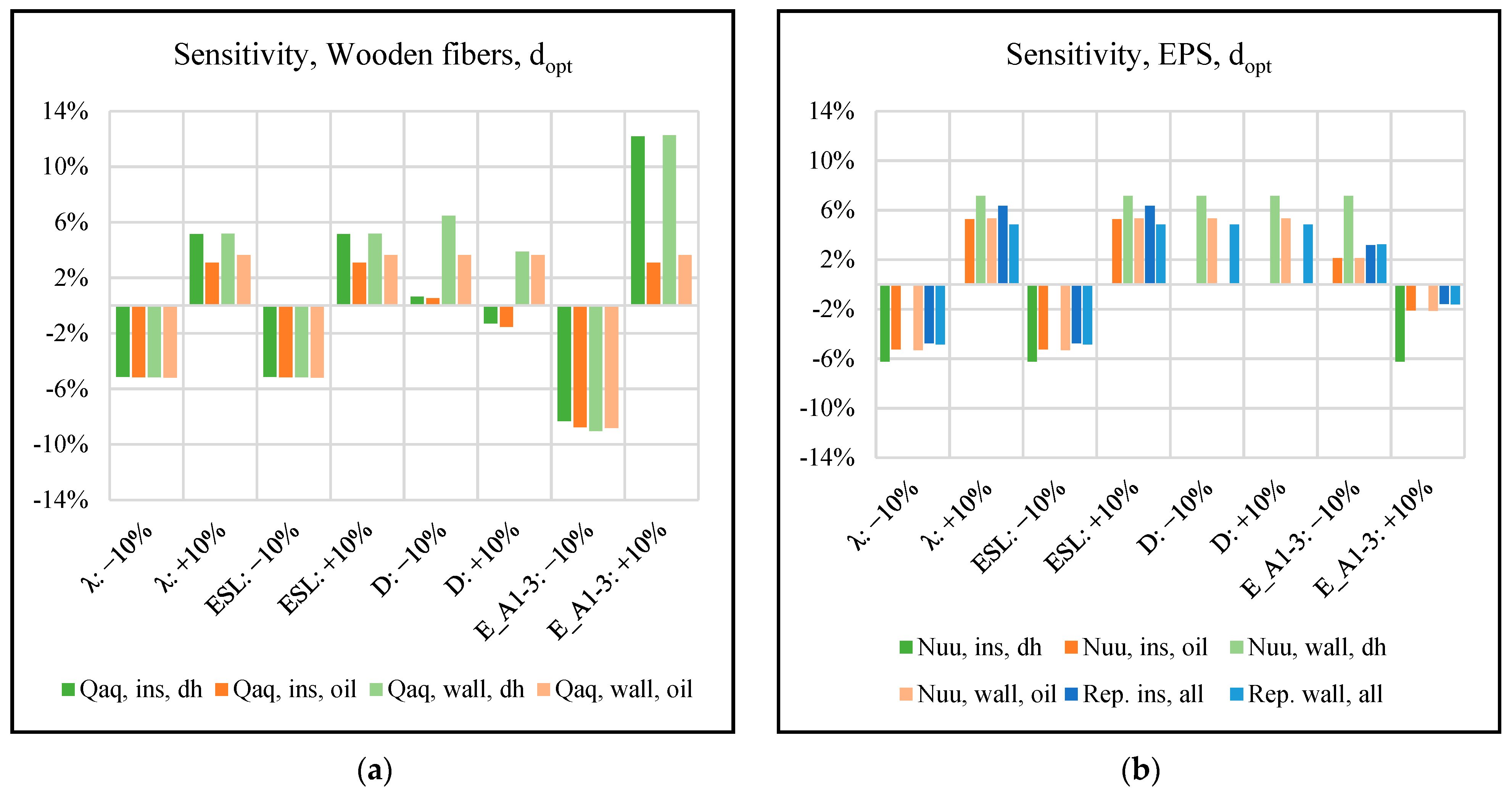
Another uncertainty of the tool is the estimation of the produced material waste and heat waste. Both were set to 5% for the results presented in this study, but in practice, the waste of insulation material will depend on the type of insulation and its handling, while the waste of heat will depend on the heating source and the type and quality of the installation. This means, that the values are likely to be different for each case. The impact of these waste fractions on the optimal insulation thickness is, however, very small, which is indicated in
Figure 7. For the Mineral wool in Qaqortoq, the
dopt for district heating increased by 5.8% when both
Wmaterial and
Wheat were increased from 5% to 15%. The emissions caused by freight of the material (
Efreight) also depends on
Wmaterial, and Equation (4) shows that it is estimated that half of the material waste is transported to the building site. By this, it is not assumed that damaged insulation is distributed to construction sites, but that some of the waste is caused by the transportation, handling, errors during construction and inevitable leftovers from reshaping the material to fit the construction. This assumption is very rough, as the quantification of waste in the construction sector is extremely challenging and influenced by uncertainties. The sensitivity analysis in
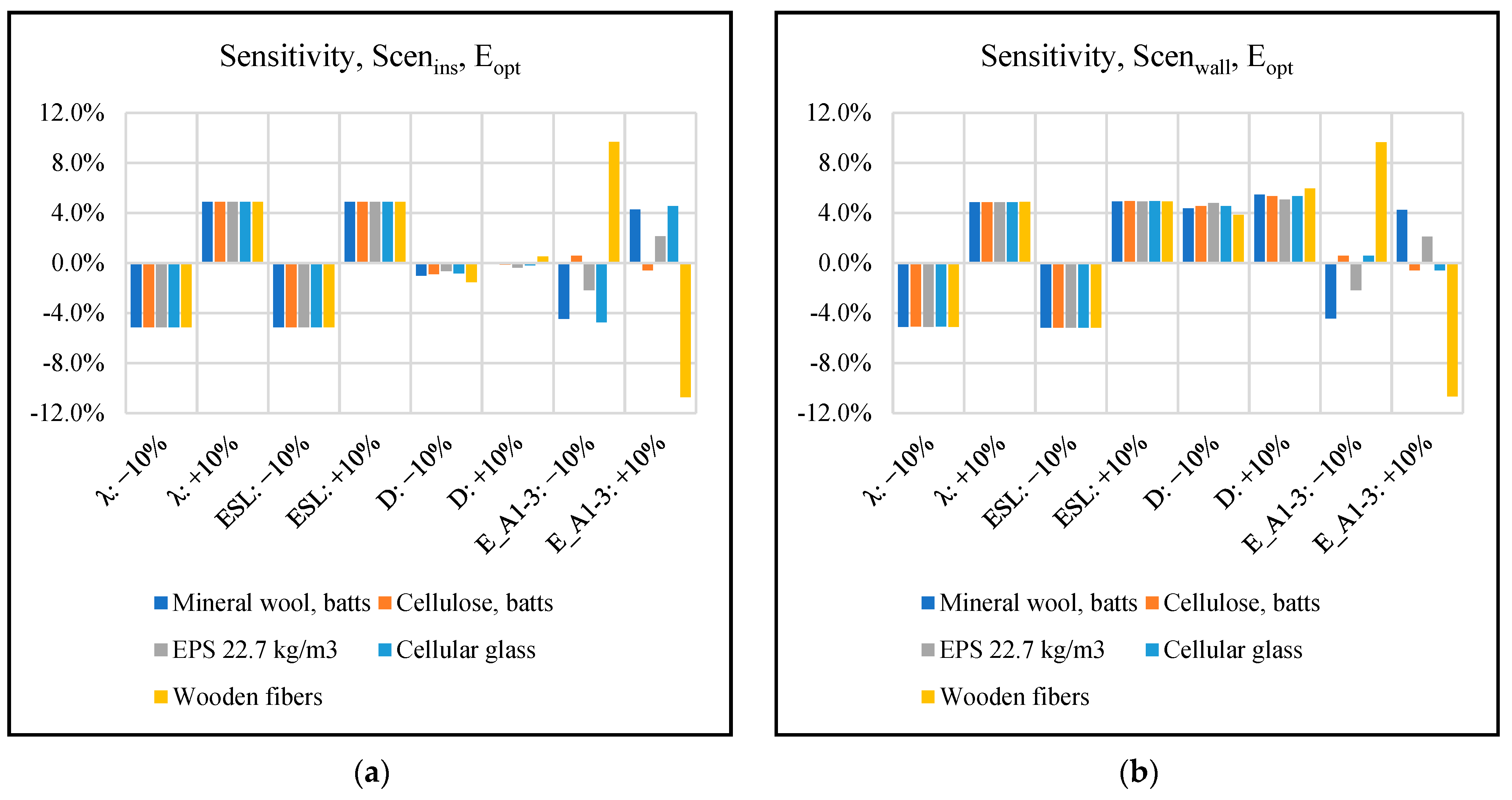
Figure 5 and
Figure 6 show that the emissions contribution from transportation is very small, especially when considering Scen
ins.
Another limitation to the system is the uncertain definition of “optimal insulation thickness”. The user must decide what the boundaries should be for the specific case. It is also an option to use all of the three success criteria presented in
Figure 8, to provide a more holistic and nuanced basis for the decision. In Dylewski et al. [
8], the research resulted in a metacriterion considering both the ecological and economic perspectives, while weighing them equally. The challenge in implementing the economy in such a simple tool as ITO is that it requires a lot of the user, in terms of researching current market values. This would likely hinder part of the target group from using the tool.
The benchmark for ITO, regarding the optimal insulation thickness, is CO
2-eq. This is a fundamental premise of the tool, and, as previously described, there are many aspects to consider. The most applied criteria are CO
2-eq and economic value, while some of the studies combine these. However, there are many other parameters to consider. The three fundamental parts of sustainability are ecology, economy and people. In none of the literature presented in
Section 1, are the people considered in more than a comment. This neglects comfort and safety. It is very common to consider ecology and economy as equally important—even in certification systems, such as DGNB [
37]. In studies that only consider ecology, it is most common to include CO
2-eq as the only parameter, however, there are many other LCA impact factors to include, such as acidification and ecotoxicity of water and ground, usage of water and the reduction in mineral resources. Including these parameters complicates the reading of the results, and the GHG in the form of CO
2-eq is a very well communicated, or even branded, measure, which most people can relate to. There is great reason to discuss whether this justifies the simplification, however, in a tool such as ITO, the users’ understanding of the results is essential, for the product to matter.
As shown in
Figure 4, incinerating the waste material emits more CO
2-eq/m
3 material than landfill. This condition can lead one to think that it is best to landfill the building waste, but as sustainability is about much more than greenhouse gases, this is not the conclusion that should be drawn from the figure.
As described in
Section 2.4, environmental development is considered, although the future conditions are uncertain. The temperature changes are being investigated thoroughly by scientists in different organizations, such as the IPCC. However, other weather phenomena may occur due to the changes in the global flow of heat and water. The impact of these possible phenomena is impossible to predict, and ITO does not consider the climate beyond the temperatures expressed by HDD. This can be considered both a strength and a weakness of the system, as it makes the system more robust to use despite uncertainties, but may exclude relevant factors. The predictions for temperature change vary both in methods and results, but the three climate scenarios included in this paper are based on acknowledged literature. As presented in
Figure 3, comparing the optimal insulation thickness for the current climate scenario with the extreme climate scenario results in only minor differences compared to the differences related to the emission factors of the locations. The proportions of climate change are uncertain and have a relatively low impact. In contrast, the energy sources have lower uncertainty and relatively high impact, due to major differences between the emission factors. For reference, the emission factor varies by a factor of 37 comparing oil and the district heating in Nuuk (consisting mainly of hydropower), while the HDD differs up to a factor of 4.4 caused by extreme climate change (for Copenhagen over 110 years). However, the energy source may change during the lifetime of the building.
ITO is designed to minimize GHG emissions, but there are many aspects to consider hen constructing a house, as was stated in the Introduction.
Section 4.2 focuses on one of them, but it is still based on the GHG emissions, while the other impacts also have important roles to play. Examples of this are comfort and buildability. The tool does not consider the practical difficulties in installing extremely thick insulation layers, which might lead to errors and problems in the construction phase. The level of comfort in a building depends on many different factors, but those that might affect the validity of an ITO analysis are comfort and daylight. In some cases, the minimum emission of GHG may be achieved with very thin layers of insulation, which might lead to cold walls during winter. Some of the results tabulated in the Results section exceeded one meter of insulation, which is far more than the 150–250 mm typically required by building regulations. This will create shadows around the windows, and therefore allow less light and heat to enter the building. Adequate light has been shown to be essential for comfort [
38], and reduced heat gain from the sun will lead to an increased demand for heating. This could be interesting to consider in the calculation but would probably require too much information about the architectural design of the building, orientation, and the window types for this to be useful in practice. The additional layers of insulation also cause reduced heat gain during sunny seasons, which can impact the need for heating and cooling. In other research, such as Ozel et al. [
3] and Axaopoulos et al. [
11], this was considered. Since ITO does not consider the need for cooling, this heat gain is less significant, however the results can be considered a worst case on this perspective.
Figure 3 showed that the optimal insulation thickness was nearly independent of the additional wall layers. This might be due to the very thick optimal insulation layers demanded by the harsh Arctic climate. In other climates, the U-value of the uninsulated wall may have a higher impact e.g., Dylewski et al. [
8] found that the optimal U-value would be independent of the uninsulated wall. The source, Ounis et al. [
12], concluded that the optimal U-value in Denmark was 0.12 W/m
2 K based on HDD
20 °C and CDD
24 °C, which led to 4348 HDD. The U-value is lower than the current building regulations that demand 0.3 W/m
2 K, and more HDD than accounted for in this study (2500). The difference is caused by the benchmark temperature when defining the days with heating demand, which was 17 °C in this study and 20 °C in the Ounis et al. study. Furthermore, the heating season might have been neglected in the other study. This is mentioned to bring awareness of the importance of the definitions and the challenges in comparing the results of different studies.
6. Conclusions
The new tool, ITO, can determine the optimal insulation thickness in walls, if this is defined as the thickness that minimizes greenhouse gas emissions. The tool uses several simplifications on how to determine energy loss, as it only considers thermal conductivity through 1 m2 wall without doors, windows, thermal bridges, etc. However, it is easy to use, and a sensitivity analysis shows that it results in reliable outputs.
The present paper clarifies the importance of insulation thickness, showing that the emissions from this parameter of the design can vary considerably, depending on the material, heating source and building location, which affects both the heating degree days and the freight distance. The output of the two scenarios, Scenins, which only considers the insulation, and Scenwall, which considers a predefined wall with multiple layers, were very similar. However, there is a significant difference between the scenarios for very thin layers of insulation, as the first centimeters of material reduce the heat loss more than the last.
The optimal insulation thickness, dopt, was found to be very HDD-dependent, while the emissions from the transport of the insulating material had limited impact, even when the distances are considerable. The sensitivity of the transportation distance, D, was found to be more vulnerable for Scenwall than for Scenins.
The system can be sensitive to processes taking place outside the system boundaries, especially when the emission factor of heat or the heating degree days is high. Different climate-change scenarios were investigated, but they caused minimal changes to the optimal insulation thickness when the Efactor was small, e.g., when district heating mainly consisting of hydropower was used. The difference in the HDD was less dependent on the climate change scenario than the location.
The tool illustrates the importance of green energy and well-considered building design. If the energy source has low CO2 emission, the optimal insulation thickness may be thinner in a cold climate than it would be in a more moderate climate with an energy source that emits more CO2.


