A Quantitative Analysis on Key Factors Affecting the Thermal Performance of the Hybrid Air-Based BIPV/T System

Abstract

Air-based BIPV/T is of significant research interest in reducing energy load and improving indoor comfort. As many factors related to meteorology, geometry and operation contribute to the thermal performance of BIPV/T, especially for one kind of hybrid air-based BIPV/T (HAB-BIPV/T), quantifying the effects of such uncertain parties is essential. In this paper, a numerical analysis was conducted regarding 13 parameters of one HAB-BIPV/T prototype. For each quantity of interest, the kernel density estimate was regarded as an approximation to the probability density function to assess uncertainty propagation. A sequential sensitivity analysis was used to quickly screen (by Morris) and exactly quantify (by Sobol’) the effects of significant variables. The surrogate model based on a back propagation neural network was employed to dramatically reduce the computational cost of Monte Carlo analysis. The results show that the uncertain inputs discussed can induce considerable fluctuations in the three quantities of interest. The most significant parameters on AUI include air inlet height, cavity thickness, air inlet velocity and number of air inlets. The outcomes of this study provide insights into the correlation between various factors and the thermal efficiency of the HAB-BIPV/T as a reference for similar design works.

1. Introduction

The International Energy Agency (IEA) identifies a precise roadmap to meeting the 2050 net zero emissions promise in its report “Net Zero by 2050: A Roadmap for the Global Energy Sector” [1], which specifically captures the crucial role of renewable energy in net zero emissions. To achieve the 4% annual reduction in energy intensity by 2030, sustained and intensified progress would be required in the application of clean and efficient energy technologies.

Recent reports have re-emphasized the essential function of the building industry in decarbonizing the global economy [2]. The path to net-zero emissions plainly entails a transition to zero-carbon-ready buildings in the construction sector. Energy efficiency and renewable energy, as the critical issues of such a transition, would imply a rapid shift to optimal technologies in all markets by 2030 [3].

Photovoltaic (PV) technology is considered a clean, flexible and cost-effective renewable energy technology that has been heavily promoted in China (China alone is responsible for 75 percent of the incremental global PV installations between 2019 and 2020 [4]). Building integrated photovoltaic/thermal (BIPV/T) systems, as a common subset of the building integrated photovoltaic (BIPV) and the photovoltaic thermal (PV/T) systems, are perceived as one of the most promising PV technologies in the construction sector [5]. BIPV refers to the integration of PV modules in the building envelope to form an exterior layer and perform cladding tasks [6]. It has been widely implemented in building roofs and facades as a major avenue for PV technology penetration in the building industry. PV/T systems combine PV and solar thermal modules with the PV modules functioning as absorbers in solar collectors. This configuration enables the simultaneous acquisition of power and low-grade heat. As a result, the BIPV/T system, in addition to generating electricity, includes a heat recovery component and has significant potential for waste heat utilization.

Conventional PV/T systems can be classified as air-based or water-based, depending on the nature of the cooling fluid. Water-based systems offer higher thermal efficiency due to their inherently superior thermophysical features [7], which can be found in more detail evaluated in Refs. [8,9,10,11]. Water-based systems, however, are subject to the risk of freezing and leakage in a dynamic environment, making them preferable to less integrated stand-alone unit forms. Furthermore, enclosure corrosion risks and high maintenance costs also obstruct the heavy application of the BIPV/T system. In contrast, an air-based system is a more cost-effective and productively sustainable option due to its easier construction and higher integration [5,12]. Therefore, this paper focuses on the innovation and evolution of air-based BIPV/T systems to refine an efficient approach to upgrading system efficiency.

The performance evaluation and improvement techniques of air-based PV/T systems are hot topics in this field of work, with the key points of interest being electrical and thermal performance [5,10,13,14], exergy efficiency [13,15,16], carbon credit [13,17] and cost-effectiveness [8,18]. Many attempts have been made to lower the working temperature of PV modules to optimize the electrical performance through enhanced heat transfer techniques; early works in this subject include Kern et al. [19], Florschuetz et al. [20] and Hegazy et al. [21]. Numerous studies have reported various experimental [6,22,23,24,25] and numerical [6,21,25,26,27] prototypes on air-based PV/T and BIPV/T systems. Yang et al. [23], for instance, developed experimental prototypes of single-entry and dual-entry BIPV/T and investigated the effects of parameters such as the number of inlets and PV transparency on thermal efficiency. This type of work, however, may be at risk of problems such as poor applicability and inadequate coverage of the prototype due to the strongly customized nature of the system configuration, test conditions or prediction scenarios [5].

A number of characteristics were investigated [5], covering system configuration (e.g., geometrical properties, function type, thermally enhanced elements), operating and testing conditions (e.g., solar irradiance, ambient temperature, wind speed, flow conditions), etc. The research on the correlation between feature metrics and building performance has been carried out, with relatively more exploration at the PV/T [10,24] and BIPV [28,29,30] levels, e.g., Chen et al. [28] revealed the uncertainty of the effect of a BIPV window at the urban neighborhood scale based on a coupled BEM-SLUCM model. Gonçalves et al. [29] proposed a simulation framework for a multi-physics field BIPV model based on a sensitivity analysis approach to investigate the effects of parameters on building performance such as convective heat transfer coefficient, airflow in the cavity and weather conditions. The paper specifically mentions that the one-at-a-time (OAT) approach is the conventional method for such work, which implies that the net effect of a single parameter is frequently evaluated, and the parameters always show parallel relationships with each other, potentially leading to incomplete performance assessment conclusions. Additionally, while typical indicators related to ventilation and material features have been validated and analyzed, the effects of the physical quantities of the heat transfer process, such as the contribution of convective heat transfer coefficient [31,32], are not yet explored as much. Although the superior performance of the BIPV/T system has been validated [33,34,35], e.g., Ref. [33] revealed that the energy efficiency of the BIPV/T system is 17–20% higher than the BIPV system under the same condition. However, the uncertainty and sensitivity analysis of the relevant parameters of the BIPV/T system has not been fully carried out. Specifically, a short list of established research has performed parameter perturbation analysis only with the mode of OAT approaches [36] or for limited target variables [23,27,37,38], and when it comes to the HAB-BIPV/T system, the systematic uncertainty analysis can be even more difficult to find.

Despite the vast amount of data available from existing studies, the work on the HAB-BIPV/T still lacks a comprehensive picture of the following points:

• Comprehensive quantitative examination of the impact of system parameters, including uncertainty propagation and sensitivity ranking: the documented volume of the analysis of the role of performance-related factors is grossly insufficient, and the conclusions are difficult to generalize due to the reality of incomplete, weakly correlated and highly limited parameters. Although global sensitivity analysis (GSA) is a preferable alternative, there are very few systematic assessment efforts based on this method due to the characteristics of various indicators and the high processing cost.
• A systematic design approach for the HAB-BIPV/T system: the HAB-BIPV/T system has few documented design cases, making it difficult to penetrate a massive market. A comprehensive thermal performance assessment considering the uncertainties from various perspectives and ranking for influential factors are still not systematically addressed. Among the existing relevant studies, deterministic experimental situations frequently struggle to establish universal mapping due to configurable aspects such as system design and operating conditions, which severely limit the reference value.

Around the analysis on uncertainty propagation and global sensitivity, we have performed an abundance of probabilistic-based multi-physics simulations of a typical HAB-BIPV/T system prototype to evaluate and quantify the impact of 13 uncertain inputs on the thermal performance of the HAB-BIPV/T system. Our objective is to answer a crucial question that occurs during the design process: for many parameters related to meteorology, geometry and operation, what is their order and law of action on thermal behavior of the HAB-BIPV/T system? The work can provide designers and potential customers with a library of model cases and critical information, and the quantitative results can help stimulate further implementation of the system in the broader market by providing design guidelines for efficiency improvement and standardization practices.

The remainder of the paper is organized as follows: Section 2 introduces the physical model and performance metrics. Section 3 depicts the configuration of multi-physics finite element model and the details of the system parameters of interest. Section 4 introduces the specific process of uncertainty quantification and the implementation of the finite element method (FEM) program. In Section 5, the uncertainty of air utilization index, PV model temperature and air outlet temperature is quantified, and the relevant factors influencing these three indicators are recognized and assessed by the multi-stage GSA methods. Finally, Section 6 discusses the main findings, limitations and future research directions.

2. Model Description and Indicators

Figure 1 presents the composition and construction of the HAB-BIPV/T system investigated. The aim of such systems is two-fold: (1) to protect the PV module from overheating, which leads to a loss of energy conversion efficiency; and (2) to allow the fresh air to be delivered inside once it is preheated by the heat exchange chamber. In this study, the model is simplified to a 2-D steady-state issue to accommodate the huge sample volume for uncertainty quantification, that is, the physical quantity transfer in the parallel direction along the wall of the system is deemed to be negligible. Due to the parameter uncertainties, it can be translated into many similar patterns in the course of the experiment, thus providing theoretical support for analogous schemes in existing research [23,39,40].

A new concept of air utilization index (AUI) is introduced in hopes of reliably characterizing the thermal behavior of the system with a single indicator, which can easily reflect the level of heat transfer between the PV module and the fresh air in the cavity. The AUI concept is an analogy from the energy utilization coefficient (EUC) in the field of air conditioning, which can characterize the energy efficiency of the airflow distribution mode. EUC is determined as the ratio of the difference in supply and exit air temperatures to the difference in supply and indoor air temperatures [41]. A higher EUC shows that the supply air is used more efficiently to warm the occupied zone, leading to greater energy efficiency [42]. For this system, the AUI is then defined as the ratio of the temperature variation of the air in the cavity to the maximum possible temperature difference, as shown in Equation (1), thus a more significant indicator implies a more adequate heat exchange, and conversely a less optimal one. Meanwhile, in addition to the proposed indicator AUI, the average temperature of the PV module and the air outlet temperature were also concerned.

$$\mathrm{AUI} =\frac{{\theta }_{outlet}-{\theta }_{inlet}}{{\theta }_{PV}-{\theta }_{inlet}}$$

(1)

where ${\theta }_{inlet}$, ${\theta }_{outlet}$ represent the inflow and outflow temperatures of air in the heating cavity, respectively, whereby the former can often be considered as an approximation to the ambient temperature; ${\theta }_{PV}$ represents the operating temperature of the PV panel.

3. Finite Element Method

3.1. Governing Equations

A coupled dual-physics model of turbulence flow and heat transfer was developed using COMSOL Multiphysics, which embeds the finite element method [43]. The continuity equation and Navier-Stokes equation were applied to characterize the turbulent flow inside the cavity as shown in Equations (2) and (3), where it is presumed to be a steady-state problem for incompressible flow with no slip at the walls conforming to the RANS (k-ε) model.

$$\rho \nabla \cdot u=0$$

(2)

$$\rho \left(u·\nabla \right)u=\nabla \cdot \left[-p·I+K\right]+F$$

(3)

where $\rho$ is the fluid density, which is considered as a function of temperature and pressure; $u$ is the velocity vector that can be decomposed into $u$, $v$ two components in the coordinate direction; $-p·I$ represents the normal force containing gravity; $K$, $F$ represent the tangential and volumetric forces during the flow, respectively.

The energy conservation equation was employed to couple turbulence and heat transfer to describe the nonisothermal flow in the cavity and heat transfer in solids. Equation (4) gives its full format, where $Q_{vd}$ and $q$ are the two key variables for coupled-physics field. The Kays–Crawford method was adopted as the heat transport turbulence model to evaluate the turbulent Schmidt number.

$$\rho c_{p}u\nabla T=-\nabla \cdot q+q_0+Q_p+Q_{vd}+\Phi$$

(4)

where $c_p$ and $T$ denote specific heat capacity and temperature, respectively; $q$ is the thermal conductivity term following Fourier’s law; $q_0$ and $Q_p$ denote inward heat flux and work performed by pressure changes, respectively, which are both equal to zero here; $Q_{vd}$ is viscous dissipation to account for flow heating; and $\Phi$ is the heat source.

3.2. Boundary Conditions

To verify the robustness of the simulation method, we first reproduced the results of an experimental study of airflow barriers for commercial aircraft [44], which reveals a good agreement. Details on this work can be found in the Appendix A. The boundary conditions tended not to be constant due to the presence of parameter uncertainties, but there existed some fixed boundary variables, including the indoor temperature (18 °C) and the static pressure at the outlet of the cavity (0 Pa). Distinct from the external side, the room temperature was set to a constant value according to the code [45] because it tends to stabilize due to the continuous use of heating facilities indoors during the winter. For the turbulent flow field, the hybrid air inlet was given a normal inflow velocity as a boundary condition, accompanied by a turbulence intensity of 0.05 and a geometry-based turbulence length scale. Therefore, in addition to geometric factors (including cavity size, inlet height and the number of inlets), the air change rate of the cavity is directly determined by the velocity and pressure boundary. As for the heat transfer field, a third-type boundary condition was set for both the inner and outer surfaces of the system. A boundary heat source, determined by solar radiation and conversion efficiency, was added to the PV panel. In this regard, the total solar energy collected by the PV panel is fully converted into electrical and thermal energy, i.e., the boundary heat source is all the radiant energy of the total solar energy collected except for the power generation use. Part of this acquired radiant energy is dissipated to the outdoors in the form of heat conduction, convection and radiation, while the other part is conducted through the PV panel and then convectively heat exchanged with the air inside the cavity. Here, the SiO₂ solar panel was regarded as a thin layer, and the heat flow through the panel was calculated using the thermal thickness approximation model with a thickness of 2 cm and thermal conductivity of 0.27 W/(m·K). Such a system configuration also allows the insulation to avoid direct contact with the outside low-temperature environment, but rather to exchange heat with the preheated air, reducing the heat dissipation from the room. The surface-to-ambient radiation can be determined by the Stefan–Boltzmann law:

$$-n\cdot q=\epsilon \sigma \left(T_{amb}^4-T^4\right)$$

(5)

where $\epsilon$ is surface emissivity; $\sigma$ is Stefan constant; $n$ is outward normal vector; $T_{amb}$ and $T$ denote ambient temperature [45] and wall surface temperature, respectively.

3.3. Control Variables

The 13 control variables shown in

Table 1. Control variables considered in relation to the ambient, design and operation of the HAB-BIPV/T system.

#	Control Variables	Abbr.	Unit	Distribution	Marginals	Ref.
1	Air cavity thickness	${\delta }_{acv}$	cm	U (5.0, 15.0)	[5, 15]	[5,23,39,40,46,47,48]
2	Insulation thickness	${\delta }_{ins}$	cm	U (4.0, 10.0)	[4, 10]	[5,23,39,40,46,47,48]
3	Insulation thermal conductivity	${\lambda }_{ins}$	W/(m·K)	U (0.5, 2.0)	[0.5, 2]	[5,23,39,40,46,47,48]
4	Masonry thickness	${\delta }_{msr}$	cm	U (11.5, 49.0)	[11.5, 49]	[5,23,39,40,46,47,48]
5	Masonry thermal conductivity	${\lambda }_{msr}$	W/(m·K)	U (0.025, 0.050)	[0.025, 0.05]	[5,23,39,40,46,47,48]
6	PV conversion efficiency	${\eta }_{pv}$	—	U (0.10, 0.25)	[0.1, 0.25]	[5,23,39,40,46,47,48]
7	Number of air inlets	$n_{ain}$	—	U (3, 8)	[3, 8]	[5,23,39,40,46,47,48]
8	Air inlet height	$H_{ain}$	cm	U (5.0, 20.0)	[5, 20]	[5,23,39,40,46,47,48]
9	Air inlet velocity	$u_{ain}$	m/s	U (0.01, 5.00)	[0.01, 5]	[5,23,39,40,46,47,48]
10	Solar radiation intensity	$I_{sol}$	W/m2	N (600, 1352)	[200, 1000]	[5,23,39,40,46,47,48]
11	Outer ambient temperature	$T_{amb}$	degC	N (0.55, 2.452)	[−6.8, 7.9]	[5,23,39,40,46,47,48]
12	Outer combined heat transfer coef.	$h_{ce}$	W/(m2·K)	N (19, 1.352)	[12, 26]	[5,23,39,40,46,47,48]
13	Inner combined heat transfer coef.	$h_{ci}$	W/(m2·K)	N (8, 0.772)	[4, 12]	[5,23,39,40,46,47,48]

Note: U (a, b) represents the uniform distribution with the lower limit of a and the upper limit of b; N (c, d²) represents the normal distribution with the mean of c and the standard deviation of d.

, consisting of parameters related to the ambient environment, geometry and operation, were fully considered in the uncertainty quantification process. Among them, the environmental factors were assumed to satisfy a normal distribution, while the factors related to geometry and operation were deemed uniformly distributed. The interval for each parameter was derived from an extensive literature review and specification search, which could cover most similar constructs. In particular, the number of air inlets $n_{ain}$ was given to the FEM program as an integer converted by round (·). In addition, the air inlet velocity $u_{ain}$ was defined as a design flow rate instead of an operating parameter to guide the selection of the appropriate power fan for flow rate control. The meteorological conditions were specified mainly for scenarios in the cold regions of China; nevertheless, it still has good generalizability due to the wide range of values.

4. Uncertainty Quantification

Uncertainty quantification consists of two main components:

1.

Uncertainty propagation analysis (UPA): the probability density function (PDF), cumulative distribution function (CDF), probability plot (PP) and cumulative distribution function (CHF) were calculated to understand in detail how the uncertainties of inputs propagate to quantities of interest.

2.

Global sensitivity analysis (GSA): the perturbation effects of uncertain inputs were ranked according to their significance and were quantified to determine how uncertainties in the quantities of interest were apportioned to the various inputs.

4.1. Probabilistic-Based UPA Method

A probabilistic-based method was applied to study the propagation of input uncertainty. No surrogate model was used in the UPA process to capture as exactly as possible how the quantities of interest were affected by the uncertain parameters, even though this might cause the additional expenditure of computational resources.

Kernel density estimation (KDE), a nonparametric method of approximating the probability distribution without any assumptions (i.e., prior knowledge) attached to the data distribution, was introduced to describe the overall trend and density distribution pattern of quantities of interest in a more specific way than the common parametric estimation methods. Suppose $X=\left\{x_1,x_2,\dots ,x_n\right\}$ are the n sample points of independently identical distribution F. For a given sample size N, the KDE of its probability density function f can be described as:

$${\widehat{f}}_h\left(x\right)=\frac{1}{nh}\sum _{i=1}^{N}K\left(\frac{x-x_i}{h}\right)$$

(6)

where $K(·)$ is a non-negative kernel function, which has an integral of 1 and a mean of 0, in accordance with the probability density property; $h$ is called the bandwidth, which is a smoothing parameter that is always positive.

From the above equation, it can be found that the estimation results obtained by the KDE method depend heavily on the choice of its kernel method and the bandwidth configuration. The selection of the kernel function tends to be more focused on its mathematical properties (i.e., solution difficulty and derivative order), while the choice of bandwidth directly determines whether the bias-variance tradeoff can be achieved.

When the optimal bandwidth is obtained, which is equivalent to minimizing $MSE\left({\widehat{f}}_h\left(x\right)\right)$, the form of the kernel function takes very little effect, and the optimal bandwidth $h_{opt}$ can be written as:

$$h_{opt}= {\kappa }_2{}^{-2/5}{\kappa }^{1/5}{\{\int {\left[f^{\left(2\right)}\left(x\right)\right]}^{2}dx\}}^{-1/5}{n}^{-1/5}$$

(7)

$${\kappa }_2=\int t^{2}K\left(t\right)dt$$

(8)

$$\kappa =\int K^2\left(t\right)dt$$

(9)

4.2. Sequential GSA Method

4.2.1. Morris Screening

Using composite GSA methods allows to greatly enhance the robustness of the conclusions and to achieve mutual complementarity with their respective characteristics [49]. Among them, Morris tends to be used as a prescreening method for parameters in sequential SA due to its higher computational efficiency to rapidly reduce the dimensionality of the uncertain parameters of interest. It uses the absolute mean and standard deviation as sensitivity scales, more specifically, the larger the former value is, implies that the input $x_i$ can induce greater variability in the quantities of interest, and the larger the latter implies that the input $x_i$ has a more significant nonlinear behavior or interaction with other variables.

4.2.2. BPNN-Based Sobol’ Method

Sobol’ indices are widely used in variance-based GSA methods due to their ability to accurately quantify the sensitivity of each input by decomposing the total variance. However, the computational resources required by this method are extremely demanding, especially for finite element models, which are inherently expensive to solve. Therefore, the surrogate model based on the BPNN was introduced as a previous step in the computation of Sobol’ indices to enrich the sample size for performing GSA. The developed BPNN is shown in Figure 2, where the output is the indicator of the system, the inputs come from the significant variables screened by Morris, and the number of hidden layers should be reasonably configured by iterative debugging. The Bayesian regularization algorithm was employed in network training, which takes longer but can result in strong adaptation for complex, limited or chaotic datasets. After iterative debugging, the model performed well when the hidden layer size was set to 12, leading to a 7 × 12 × 3 BPNN. Meanwhile, due to the modest hidden layer size, the activation function can be chosen broadly, which was specified as the sigmoid symmetric transfer function in this study. It is worth noting that both the Sobol’ method and BPNN training require uncorrelated or minimally correlated inputs, thus a correlation test needs to be conducted on the parameters in advance (as Section 5.3.1).

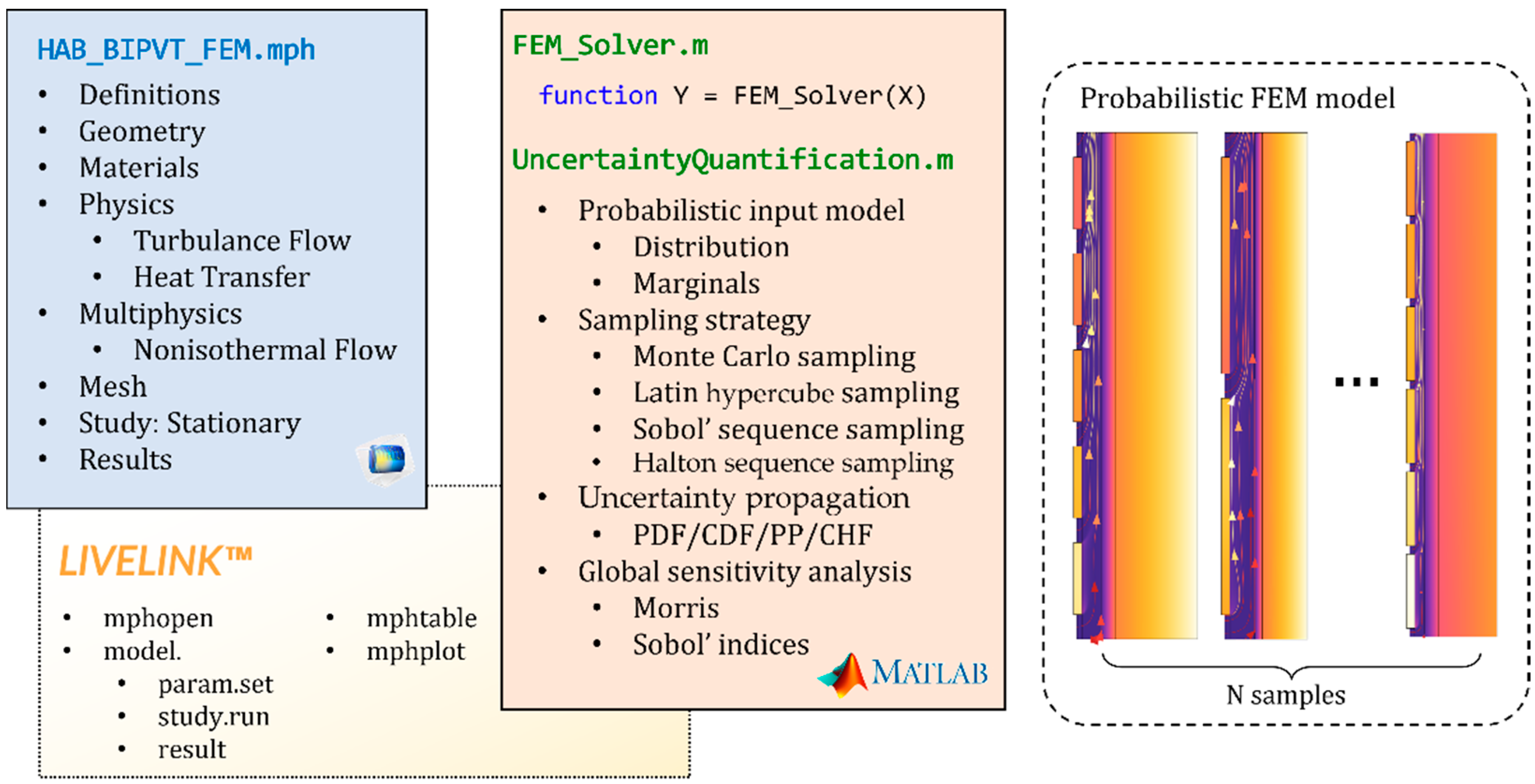
4.3. Implementation of Uncertainty Quantification in FEM Program

The FEM program can often be well suited to calculate deterministic inputs and even some orthogonal experimental tasks. To perform simulations with parametric uncertainties, COMSOL Multiphysics was linked to MATLAB for co-simulation through the Livelink interface for data interaction. In this way, the COMSOL solver can be invoked by MATLAB, which enables most of the operations to be performed on the identical platform, such as the configuration and generation of sample sets, the extraction and definition of parameters, as well as the evaluation and analysis of quantities of interest. The detailed implementation of the process is illustrated in Figure 3.

5. Result and Discussion

5.1. Uncertainty Propagation

To characterize the effect of uncertain inputs on the output comprehensively, a mixed sampling strategy was employed, which involved Monte Carlo sampling, Latin hypercube sampling, Sobol’ sequence sampling and Halton sequence sampling. Each strategy provided 1300 samples for UPA, thus yielding a total sample capacity of 5200. Here, in addition to the previously proposed indicator AUI, the average temperature of the PV module (TPV) and the air outlet temperature (TAO) were also considered as quantities of interest. The uncertainty of the quantities of interest was described by the normal kernel function with optimal bandwidth as shown in Figure 4. Probability density, approximated by KDE, was used to describe the probability that the output value of uncertainty is around a certain value point. As an integral of the PDF, the cumulative probability can completely describe the probability distribution of a random variable. From the results, the 13 uncertain inputs in focus can lead to significant fluctuations of 0.456, 29.138 °C and 14.680 °C for AUI, TPV and TAO, respectively. From the probability plot, it can be seen that there are significant differences in the distribution characteristics of the three indicators, especially the AUI, which shows a severe left-skewed distribution. For the normal distribution, the mean values of the three are 0.080, 7.090 °C, 1.088 °C, and the corresponding standard deviations are 0.039, 4.198 °C, 2.464 °C, respectively. Furthermore, cumulative probability enables designers to determine the threshold of any probability and thus set specific risk levels for system reliability from a safety and economic perspective. Similarly, the cumulative hazard, which provides the total accumulated risk of encountering the event of interest that has been obtained, has a similar function to assist in avoiding specific events, such as keeping the average temperature of the PV module below a specified value to ensure a high level of power generation efficiency.

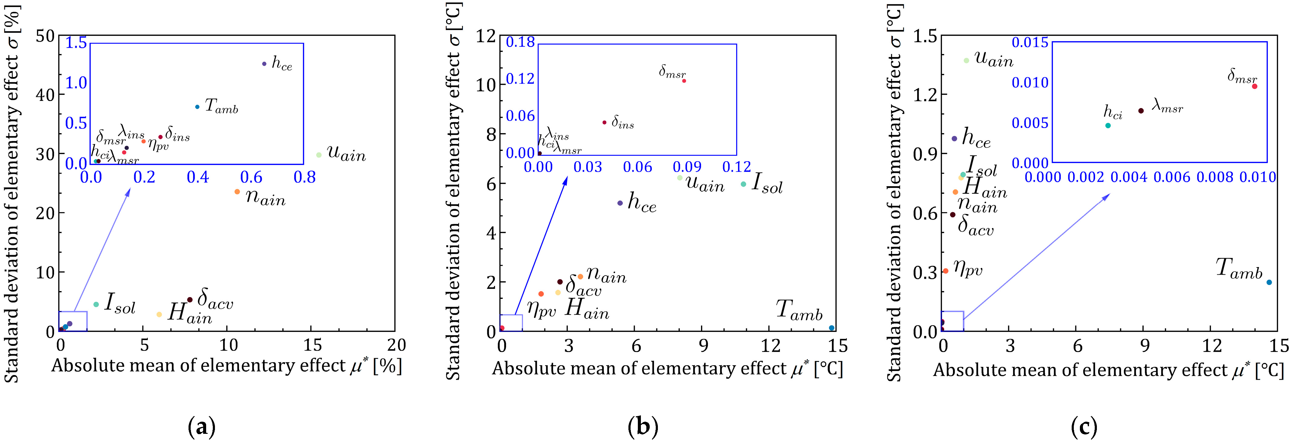
5.2. Parameter Screening by Morris

Using a trajectory-based sampling technique, the sampling size requirement of Morris can be reduced to (M + 1) r, where the repeated times r is often taken between 5 and 15, and here the input dimension M is equal to 13. The FEM solver was called for a total of 196 calculations in this step of GSA. To efficiently screen from qualitative results, the sensitivity of AUI, TPV and TAO to each uncertain input was compared and analyzed. During GSA with multiple outputs, inputs that consistently ranked lower were identified as minor variables and were not involved in the next step of the analysis. Figure 5 shows the Morris analysis results for AUI, TPV and TAO. Surprisingly, the top four parameters that have a significant impact on AUI are all design-related parameters rather than ambient ones. For the other two indicators, the outdoor ambient parameters, including $T_{amb}$, $I_{sol}$ and $h_{ce}$, always stand out, especially for $T_{amb}$, which separately creates the strongest perturbation to TPV and TAO. This suggests, to some extent, that outdoor ambient parameters do have a prominent effect on the thermal behavior of the HAB-BIPV/T system, e.g., it is easily understood that a lower ambient temperature naturally leads to a significant decrease in TPV and TAO, yet it does not imply superior efficiency at this point, due to the presence of AUI in a relative magnitude between temperature differences. Despite the significant differences in the GSA results of the three regarding each input, $u_{ain}$, $n_{ain}$, ${\delta }_{acv}$, $H_{ain}$, $I_{sol}$, $h_{ce}$ and $T_{amb}$ are consistently ranked in the top seven, while the remaining variables consisting of ${\delta }_{ins}$, ${\eta }_{pv}$, ${\lambda }_{ins}$, ${\delta }_{msr}$, ${\lambda }_{msr}$ and $h_{ci}$ display limited influence in the results and are thus screened out from the subsequent analysis.

5.3. Sobol’ Indices Based on BPNN Model

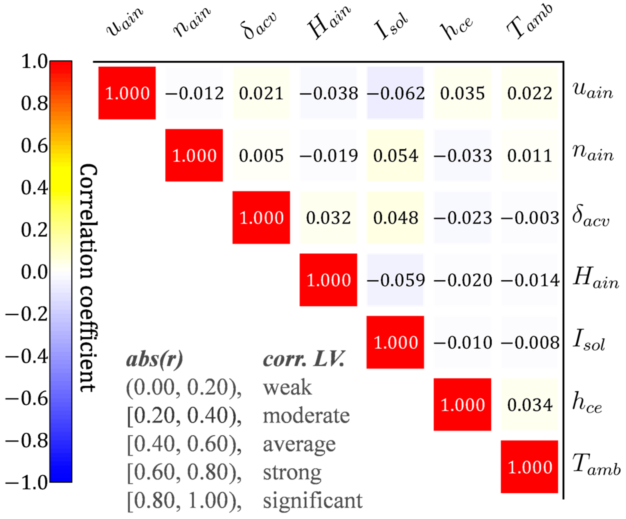
5.3.1. Parameter Correlation Analysis

Pearson stays the most common evaluation approach when it comes to parameter correlation studies. However, using Pearson still has many limitations on the nature of the variables, i.e., it requires data to be continuous, linearly correlated and normally distributed (if a t-test is applied), and thus is regarded as not applicable to this study. In contrast, the Spearman correlation coefficient used in this section is more tolerant to the data conditions and thus has a broader range of applicability. The correlations between 1050 sets of input variables obtained by the Latin hypercube sampling (LHS) technique were analyzed, and the results were calculated as shown in Figure 6. The results show that each pair of parameters shows a very weak correlation, to the extent that they can be considered uncorrelated. This provides a theoretical premise for the use of the BPNN model and Sobol’ method.

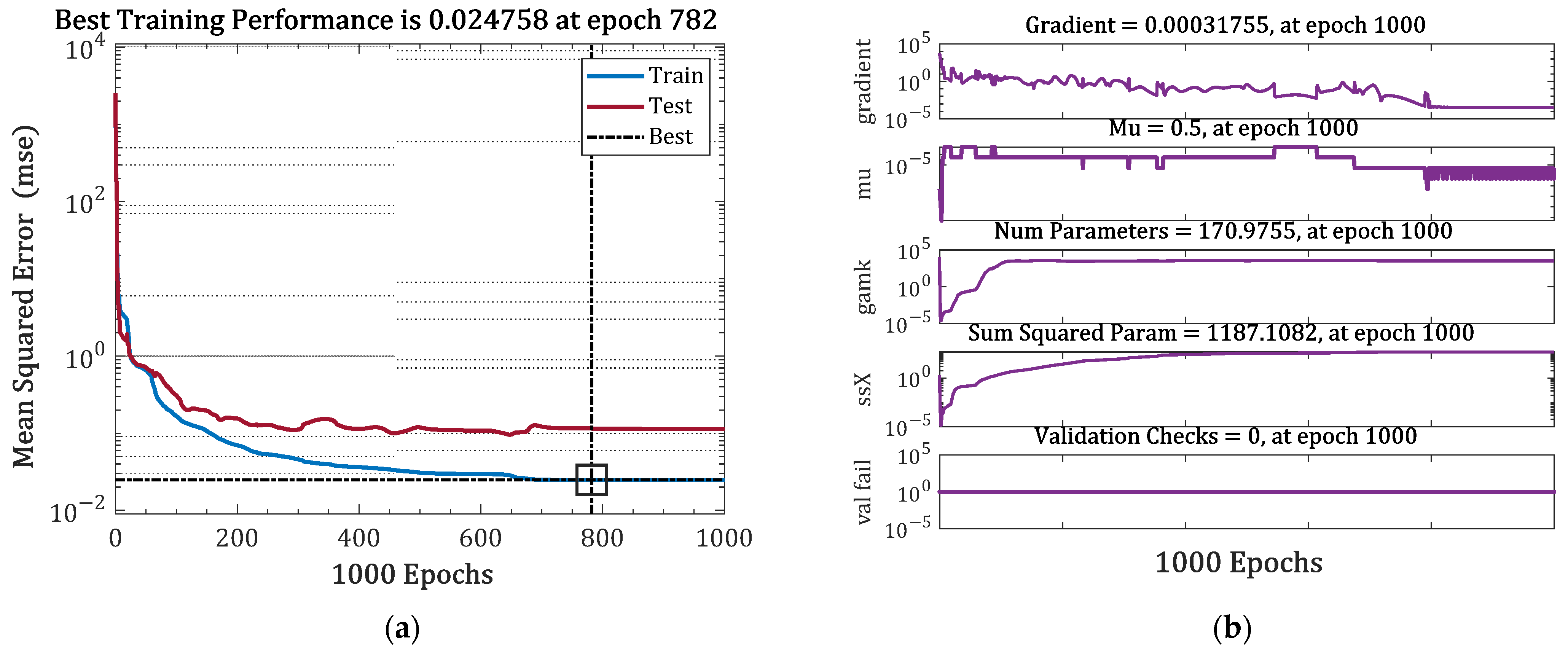
5.3.2. BPNN-Based Surrogate Model

The 1050 datasets for training the BPNN model were provided by LHS. A total of 840 samples (80% of total) were set as the training set and the remaining samples were equally divided into two groups for validation and testing, respectively. Figure 7 shows the details of the resulting surrogate model. The accuracy of the model is again verified by the lower MSE (0.041) and the larger R (0.998) obtained by conducting additional tests on the model with an additional 500 sets of data. Thus, the surrogate model is considered as an alternative to the FEM program to accomplish extensive calculations for uncertain inputs in the next session of GSA.

To further manifest the robustness of the trained BPNN model, the trending of indicators with significant inputs was shown in

Table 2. The trends of quantities of interest with seven significant variables in the given intervals.

Control Variables	Indicators
	AUI	TPV	TAO
$\mathrm{Air} \mathrm{inlet} \mathrm{velocity} u_{ain}$	●●	●●●	●
$\mathrm{Number} \mathrm{of} \mathrm{air} \mathrm{inlets} n_{ain}$	●●	●●●	●
$\mathrm{Air} \mathrm{cavity} \mathrm{thickness} {\delta }_{acv}$	●●●	○○	●
$\mathrm{Air} \mathrm{inlet} \mathrm{height} H_{ain}$	●●●	●●	●
$\mathrm{Solar} \mathrm{radiation} \mathrm{intensity} I_{sol}$	●	○○○	○○
$\mathrm{Outer} \mathrm{combined} \mathrm{heat} \mathrm{transfer} \mathrm{coef}. h_{ce}$	○	●●●	○○
$\mathrm{Outer} \mathrm{ambient} \mathrm{temperature} T_{amb}$	●	○○○	○○

● represents that the indicator is trending opposite to the variable, while ○ represents that both are trending the same. The number of symbols indicates the impact of the variable.

, which was compared with the outcome of similar studies. Among them, Yang and Athienitis [23] concentrated on thermal efficiency and outlet air temperature and reported their trends with air mass flow rate, wind speed and number of inlets; whereas Rounis [27] not only presented the variation of PV panel temperature with these three parameters but also paid additional attention to the effect of the channel gap. The conclusions we reached are in good agreement and complementary to Ref. [27], but there are still some differences in conclusions with Ref. [23] in terms of air inlet number and air mass flow rate. This is due to some differences between the studies themselves: (1) in Ref. [23], the system was tested at a tilt angle of 45°, while in Ref. [27] and this study, the vertical system was concerned; (2) in Ref. [23], the thermal efficiency was calculated with respect to the mass flow rate, while in this study, it was expressed as a ratio of temperature differences due to the consideration of more factors that can affect the mass flow rate; (3) in terms of the number of air inlets, Ref. [23] focuses on whether dual inlets can improve the system efficiency compared to the single inlet, while this paper focuses on a system with more inlets, which makes the conclusions of the two papers complementary. These trends, however, are only valid for the intervals given in this study, which can describe the dominant system forms due to their nonlinearity.

5.3.3. Sensitivity Quantification

The quantification of parameter sensitivity was captured by Sobol’ indices, where first-order indices represent the relative contribution of each variable to the total variance, and total indices can explain the interaction of variables as the sum of all Sobol’ indices. We compared the Sobol’ indices derived from four different sampling strategies in this step of GSA, and the sample size for each strategy was set to 1E5, which means that for seven inputs, the total cost of each strategy was 9E5 evaluations of the computational model. Figure 8 indicates the differences in the first-order and total Sobol’ indices obtained based on the four sampling strategies. In general, although the four strategies show different quantitative results, the determination of the relative magnitude of these seven variables remains largely consistent. The comparison of the two indices also shows that the interaction between the inputs is limited to the extent that it does not cause variations in the parameter rankings. The GSA at this step reveals that the AUI is much less sensitive to environment-related factors (including $I_{sol}$, $T_{amb}$, $h_{ce}$) than to the design-related ones. Compared with the results shown in the previous step of Morris, Sobol’ indices show general consistency in the ranking of uncertain inputs even though a slight gap in detail exists due to the lower calculation effort of Morris. This deviation can also be attributed to a strong nonlinear effect; however, the Morris outcomes might be considered informative as they remain consistent with the Sobol’ method in overall terms as well as complementary to the Sobol’ indices. Among the four design-related parameters, the significance ranking of the parameter effects is $H_{ain}$ greater than ${\delta }_{acv}$ greater than $u_{ain}$ greater than $n_{ain}$. Even though changing the height and number of air inlets can significantly enhance the thermal efficiency, it may not be the best strategy from the perspective of electrical efficiency because they always affect the temperature of the PV module, thus a more in-depth and comprehensive reliability-based optimization study is needed while considering both the electrical and thermal efficiency. Among the four most significant parameters, appropriately reducing the cavity thickness can improve thermal efficiency and reduce the temperature of the PV panel, making it the most cost-effective measure. At this point, the four parameters most sensitive to the AUI are identified from the initial 13 parameters, and all of them relate to the fluid flow state in the cavity, which is the most prominent difference from the common BIPV/T system. In previous related parametric studies, this point has never been clearly quantified, hence, the results could not be compared effectively. However, this quantitative conclusion can still be deemed valid because we controlled the bias as much as possible by large volume simulation, hybrid sampling strategies and multi-stage GSA. It also suggests that the HAB-BIPV/T system is more prone to further optimize its thermal performance by adjusting the parameters due to the strong sensitivity of the AUI on design-related parameters.

6. Conclusions

Both deterministic models and orthogonal experimental methods provide very limited decision support for the BIPV/T design, due to the interference of excessive inevitable subjective factors. For the HAB-BIPV/T system, which involves more complex variables, it is even more difficult to rationally decompose the optimal design target to the parameter level. Uncertainty quantification, on the other hand, provides a reference solution to this challenge by explaining the interaction behavior between inputs and outputs. Therefore, this paper conducts a study on the thermal performance of the HAB-BIPV/T system from the perspectives of uncertainty propagation and sensitivity.

A novel indicator for evaluating the thermal efficiency of the HAB-BIPV/T system, AUI, was proposed as the main quantity of interest. Meanwhile, the average temperature of the PV module and the air outlet temperature were also accorded due attention. The uncertainty propagation of 13 inputs was quantified using a probability-based approach with a hybrid sampling strategy. It can be seen from PDF, CDF, PP, CHF that the discussed 13 uncertainty inputs can induce significant fluctuations in the three quantities of interest. Furthermore, the obtained results can help designers to understand the reliability of the system by calculating the risk threshold.

A sequential GSA method consisting of Morris and Sobol’ indices helped to screen and quantitatively rank numerous uncertain parameters. According to the identification results of the multi-output Morris, six variables, including the thickness and thermal conductivity of insulation, the thickness and thermal conductivity of masonry layer, inner combined heat transfer coefficient and PV conversion efficiency, always affect the quantities of interest at a limited level and are thus screened out. Before calculating Sobol’ indices based on the BPNN model, the mutual uncorrelation between parameters was first validated. First-order and total Sobol’ indices were then given separately based on four different sampling strategies. After two rounds of GSA, the four parameters with the most significant effects on AUI include air inlet height, cavity thickness, air inlet velocity and number of air inlets. This again proves that such HAB-BIPV/T systems should not be fully referenced to conventional systems when making design decisions, as its thermal behavior has been influenced by its unique air-cooling-related parameters far more than other design-related parameters, and even more than ambient parameters. It provides the theoretical support for achieving rapid and efficient optimization of the HAB-BIPV/T system. However, it should be noted that since the FEM model was developed in two dimensions, the physical quantities in the third dimension were assumed to be uniformly distributed both for heat transfer and flow physics. If the flow-thermal behavior of the model cannot be neglected in the third dimension, the conclusions drawn may be biased to some extent.

Aiming to provide user-friendly application support to designers, further research focuses on encapsulating the full-flow uncertainty quantification code for the system into a FEM program, such as COMSOL Multiphysics, so that the whole work can be presented in a form-based interface to meet designers’ individual needs for parameter configurations in the uncertainty quantification process.

References

1. IEA. Net Zero by 2050 A Roadmap for the Global Energy Sector; IEA: Pairs, France, 2021. [Google Scholar]
2. IEA. Roadmap for Energy-Efficient Buildings and Construction in the Association of Southeast Asian Nations; IEA: Paris, France, 2022. [Google Scholar]
3. IEA. Tracking Buildings 2021; IEA: Pairs, France, 2021. [Google Scholar]
4. IEA. Solar PV; IEA: Pairs, France, 2021. [Google Scholar]
5. Rounis, E.D.; Athienitis, A.; Stathopoulos, T. Review of Air-Based PV/T and BIPV/T Systems-Performance and Modelling. Renew. Energy 2021, 163, 1729–1753. [Google Scholar] [CrossRef]
6. Yang, T.; Athienitis, A.K. A Study of Design Options for a Building Integrated Photovoltaic/Thermal (BIPV/T) System with Glazed Air Collector and Multiple inlets. Sol. Energy 2014, 104, 82–92. [Google Scholar] [CrossRef]
7. Tripanagnostopoulos, Y.; Nousia, T.; Souliotis, M.; Yianoulis, P. Hybrid Photovoltaic/Thermal Solar systems. Sol. Energy 2002, 72, 217–234. [Google Scholar] [CrossRef]
8. Brahim, T.; Jemni, A. Economical Assessment and Applications of Photovoltaic/Thermal Hybrid Solar Technology: A Review. Sol. Energy 2017, 153, 540–561. [Google Scholar] [CrossRef]
9. Sultan, S.M.; Ervina Efzan, M.N. Review on Recent Photovoltaic/Thermal (PV/T) Technology Advances and Applications. Sol. Energy 2018, 173, 939–954. [Google Scholar] [CrossRef]
10. Al-Waeli, A.H.A.; Sopian, K.; Kazem, H.A.; Chaichan, M.T. Photovoltaic/Thermal (PV/T) Systems: Status and Future prospects. Renew. Sustain. Energy Rev. 2017, 77, 109–130. [Google Scholar] [CrossRef]
11. Maghrabie, H.M.; Abdelkareem, M.A.; Al-Alami, A.H.; Ramadan, M.; Mushtaha, E.; Wilberforce, T.; Olabi, A.G. State-of-the-Art Technologies for Building-Integrated Photovoltaic Systems. Buildings 2021, 11, 383. [Google Scholar] [CrossRef]
12. Chaibi, Y.; El Rhafiki, T.; Simón-Allué, R.; Guedea, I.; Luaces, S.C.; Gajate, O.C.; Kousksou, T.; Zeraouli, Y. Air-Based Hybrid Photovoltaic/Thermal Systems: A Review. J. Clean. Prod. 2021, 295, 126211. [Google Scholar] [CrossRef]
13. Agrawal, S.; Tiwari, G.N. Overall Energy, Exergy and Carbon Credit Analysis by Different Type of Hybrid Photovoltaic Thermal Air Collectors. Energy Convers. Manag. 2013, 65, 628–636. [Google Scholar] [CrossRef]
14. Hussain, F.; Othman, M.Y.H.; Sopian, K.; Yatim, B.; Ruslan, H.; Othman, H. Design Development and Performance Evaluation of Photovoltaic/Thermal (PV/T) Air Base Solar Collector. Renew. Sustain. Energy Rev. 2013, 25, 431–441. [Google Scholar] [CrossRef]
15. Yazdanifard, F.; Ameri, M. Exergetic Advancement of Photovoltaic/Thermal Systems (PV/T): A Review. Renew. Sustain. Energy Rev. 2018, 97, 529–553. [Google Scholar] [CrossRef]
16. Das, D.; Kalita, P.; Roy, O. Flat Plate Hybrid Photovoltaic-Thermal (PV/T) System: A Review on Design and Development. Renew. Sustain. Energy Rev. 2018, 84, 111–130. [Google Scholar] [CrossRef]
17. Liu, K.; Zhu, B.; Chen, J.; Liu, K.; Zhu, B.; Chen, J. Low-Carbon Design Path of Building Integrated Photovoltaics: A Comparative Study Based on Green Building Rating Systems. Buildings 2021, 11, 469. [Google Scholar] [CrossRef]
18. Zondag, H.A. Flat-Plate PV-Thermal Collectors and Systems: A Review. Renew. Sustain. Energy Rev. 2008, 12, 891–959. [Google Scholar] [CrossRef] [Green Version]
19. Kern, E.C., Jr.; Russell, M.C. Combined Photovoltaic and Thermal Hybrid Collector Systems. In Proceedings of the Combined Photovoltaic and Thermal Hybrid Collector Systems, Washington, DC, USA, 5 June 1978. [Google Scholar]
20. Florschuetz, L.W. Extension of the Hottel-Whillier Model to the Analysis of Combined Photovoltaic/Thermal Flat Plate Collectors. Sol. Energy 1979, 22, 361–366. [Google Scholar] [CrossRef]
21. Hegazy, A.A. Comparative Study of the Performances of Four Photovoltaic/Thermal Solar Air Collectors. Energy Convers. Manag. 2000, 41, 861–881. [Google Scholar] [CrossRef]
22. Rounis, E.D.; Athienitis, A.K.; Stathopoulos, T. BIPV/T Curtain Wall Systems: Design, Development and Testing. J. Build. Eng. 2021, 42, 103019. [Google Scholar] [CrossRef]
23. Yang, T.; Athienitis, A.K. Experimental Investigation of a Two-Inlet Air-Based Building Integrated Photovoltaic/Thermal (BIPV/T) System. Appl. Energy 2015, 159, 70–79. [Google Scholar] [CrossRef]
24. Qureshi, U.; Baredar, P.; Kumar, A. Effect of Weather Conditions on the Hybrid Solar PV/T Collector in Variation of Voltage and Current. Int. J. Res. 2014, 1, 872–879. [Google Scholar]
25. Li, G.; Pei, G.; Ji, J.; Yang, M.; Su, Y.; Xu, N. Numerical and Experimental Study on A PV/T System with Static Miniature Solar Concentrator. Sol. Energy 2015, 120, 565–574. [Google Scholar] [CrossRef]
26. Athienitis, A.K.; Barone, G.; Buonomano, A.; Palombo, A. Assessing Active and Passive Effects of Façade Building Integrated Photovoltaics/Thermal Systems: Dynamic Modelling and Simulation. Appl. Energy 2018, 209, 355–382. [Google Scholar] [CrossRef]
27. Rounis, E.D.; Athienitis, A.K.; Stathopoulos, T. Multiple-Inlet Building Integrated Photovoltaic/Thermal System Modelling Under Varying Wind and Temperature Conditions. Sol. Energy 2016, 139, 157–170. [Google Scholar] [CrossRef] [Green Version]
28. Chen, L.; Yang, J.; Li, P. Modelling the Effect of BIPV Window in the Built Environment: Uncertainty and Sensitivity. Build. Environ. 2022, 208, 108605. [Google Scholar] [CrossRef]
29. Gonçalves, J.E.; van Hooff, T.; Saelens, D. Understanding the Behaviour of Naturally-Ventilated BIPV Modules: A Sensitivity Analysis. Renew. Energy 2020, 161, 133–148. [Google Scholar] [CrossRef]
30. Liu, X.; Wu, Y.; Hou, X.; Liu, H. Investigation of the Optical Performance of a Novel Planar Static PV Concentrator with Lambertian Rear Reflectors. Buildings 2017, 7, 88. [Google Scholar] [CrossRef] [Green Version]
31. Mirsadeghi, M.; Cóstola, D.; Blocken, B.; Hensen, J.L.M. Review of External Convective Heat Transfer Coefficient Models in Building Energy Simulation Programs: Implementation and Uncertainty. Appl. Therm. Eng. 2013, 56, 134–151. [Google Scholar] [CrossRef]
32. Montazeri, H.; Blocken, B. New Generalized Expressions for Forced Convective Heat Transfer Coefficients at Building Facades and Roofs. Build. Environ. 2017, 119, 153–168. [Google Scholar] [CrossRef] [Green Version]
33. Agrawal, B.; Tiwari, G.N. Life Cycle Cost Assessment of Building Integrated Photovoltaic Thermal (BIPVT) Systems. Energy Build. 2010, 42, 1472–1481. [Google Scholar] [CrossRef]
34. Delisle, V.; Kummert, M. Cost-Benefit Analysis of Integrating BIPV-T Air Systems Into Energy-Efficient Homes. Sol. Energy 2016, 136, 385–400. [Google Scholar] [CrossRef]
35. Debbarma, M.; Sudhakar, K.; Baredar, P. Comparison of BIPV and BIPVT: A Review. Resour.-Effic. Technol. 2017, 3, 263–271. [Google Scholar] [CrossRef]
36. Yang, S.; Fiorito, F.; Prasad, D.; Sproul, A.; Cannavale, A. A Sensitivity Analysis of Design Parameters of BIPV/T-DSF in Relation to Building Energy and Thermal comfort Performances. J. Build. Eng. 2021, 41, 102426. [Google Scholar] [CrossRef]
37. Yang, S.; Cannavale, A.; Di Carlo, A.; Prasad, D.; Sproul, A.; Fiorito, F. Performance Assessment of BIPV/T Double-Skin Façade for Various Climate Zones in Australia: Effects on Energy Consumption. Sol. Energy 2020, 199, 377–399. [Google Scholar] [CrossRef]
38. Assoa, Y.B.; Sauzedde, F.; Boillot, B. Numerical Parametric Study of the Thermal and Electrical Performance of A BIPV/T Hybrid Collector for Drying Applications. Renew. Energy 2018, 129, 121–131. [Google Scholar] [CrossRef]
39. Bambara, J.; Athienitis, A.K.; O’Neill, B. Design and Performance of a Photovoltaic/Thermal System Integrated with Transpired Collector. Ashrae Trans. 2011, 117, 403–410. [Google Scholar]
40. Rounis, E.; Kruglov, O.; Ioannidis, Z.; Athienitis, A.; Stathopoulos, T. Experimental Investigation of BIPV/T Envelope System with Thermal Enhancements for Roof and Curtain Wall Applications. In Proceedings of the 34th European PV Solar Energy Conference (EU PVSEC), Amsterdam, The Netherlands, 25–29 September 2017. [Google Scholar]
41. Wan, T.; Bai, Y.; Wu, L.; He, Y. Multi-criteria decision making of integrating thermal comfort with energy utilization coefficient under different air supply conditions based on human factors and 13-value thermal comfort scale. J. Build. Eng. 2021, 39, 102249. [Google Scholar] [CrossRef]
42. Zhang, S.; Lin, Z.; Ai, Z.; Wang, F.; Cheng, Y.; Huan, C. Effects of operation parameters on performances of stratum ventilation for heating mode. Build. Environ. 2019, 148, 55–66. [Google Scholar] [CrossRef]
43. Pepper, D.W.; Heinrich, J.C. The Finite Element Method: Basic Concepts and Applications with MATLAB®, MAPLE, and COMSOL; CRC Press: Boca Raton, FA, USA, 2017. [Google Scholar]
44. Zhang, T.; Tian, L.; Lin, C.-H.; Wang, S. Insulation of commercial aircraft with an air stream barrier along fuselage. Build. Environ. 2012, 57, 97–109. [Google Scholar] [CrossRef]
45. GB 50176-2016; Code for Thermal Design of Civil Building. Ministry of Housing and Urban-Rural Development of the People’s Republic of China: Beijing, China, 2017.
46. Martín-Chivelet, N.; Kapsis, K.; Wilson, H.R.; Delisle, V.; Yang, R.; Olivieri, L.; Polo, J.; Eisenlohr, J.; Roy, B.; Maturi, L.; et al. Building-Integrated Photovoltaic (BIPV) Products and Systems: A Review of Energy-Related Behavior. Energy Build. 2022, 262, 111998. [Google Scholar] [CrossRef]
47. Duffie, J.A.; Beckman, W.A.; Blair, N. Solar Engineering of Thermal Processes, Photovoltaics and Wind; John Wiley & Sons: Hoboken, NJ, USA, 2020. [Google Scholar]
48. Chen, Y.; Athienitis, A.K.; Galal, K. Modeling, Design and Thermal Performance of a BIPV/T System Thermally Coupled with a Ventilated Concrete Slab in a Low Energy Solar House: Part 1, BIPV/T System and House Energy Concept. Sol. Energy 2010, 84, 1892–1907. [Google Scholar] [CrossRef]
49. Wei, T. A Review of Sensitivity Analysis Methods in Building Energy Analysis. Renew. Sustain. Energy Rev. 2013, 20, 411–419. [Google Scholar] [CrossRef]
Figure 1. Schematic view of the components of the HAB-BIPV/T system.
Buildings 12 01135 g001
Figure 2. Graphical diagram of the 7 × 12 × 3 back propagation neural network (BPNN).
Buildings 12 01135 g002
Figure 3. Implementation of uncertainty quantification in FEM program.
Buildings 12 01135 g003
Figure 4. Probability distribution of three quantities of interest induced by 5200 sets of uncertain inputs: (a) Density and cumulative probability; (b) Probability plot; (c) Cumulative hazard.
Buildings 12 01135 g004
Figure 5. Absolute mean and standard deviation for each input parameter in global screening: (a) AUI; (b) TPV; (c) TAO.
Buildings 12 01135 g005
Figure 6. Verification based on Spearman correlation coefficient of parameter irrelevance for evaluating Sobol’ indices.
Buildings 12 01135 g006
Figure 7. Specific information of BPNN-based surrogate model for sensitivity quantification: (a) Performance (MSE); (b) Training state; (c) Error histogram; (d) Regression.
Buildings 12 01135 g007aBuildings 12 01135 g007b
Figure 8. The difference between first-order and total Sobol’ indices obtained based on four sampling strategies: (a) first-order Sobol’ indices; (b) total Sobol’ indices.
Buildings 12 01135 g008