A Novel Combination of PCA and Machine Learning Techniques to Select the Most Important Factors for Predicting Tunnel Construction Performance


 ,
,  ,
,  ,
,  and
and
Abstract
:1. Introduction
2. Methodology Background
2.1. ANN
2.2. ABC
- ⮚
- Food source selection: In this stage, bee colonies will be searched for different sources of food and their characteristics. Some include nectar taste, the distance between bee colony and the hive, and energy richness [64].
- ⮚
2.3. Principal Component Analysis (PCA)
3. Materials and Methods
3.1. Case Study and Data Collection
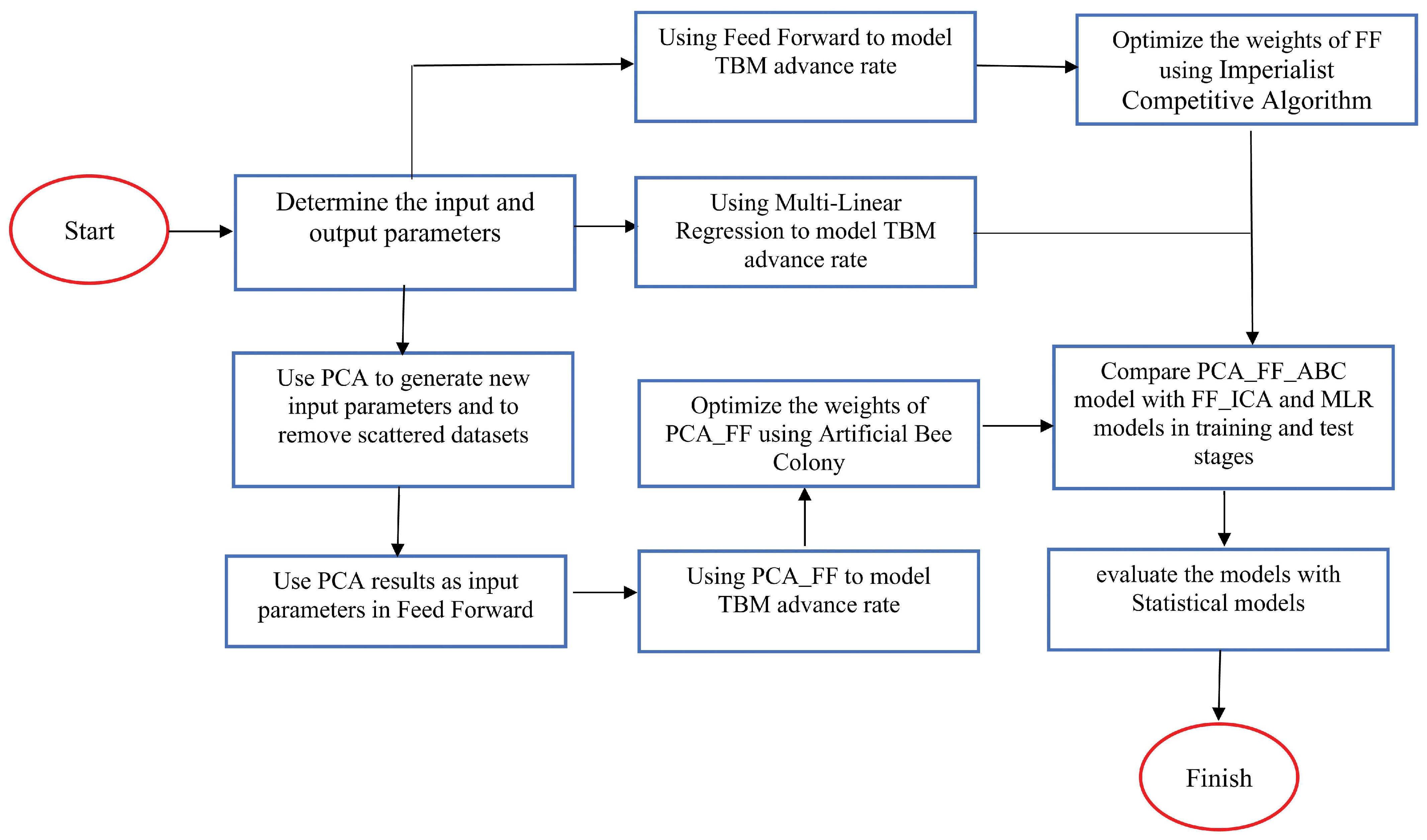
3.2. Study Steps
3.3. Research Methodology
3.4. Validation of the Developed Model
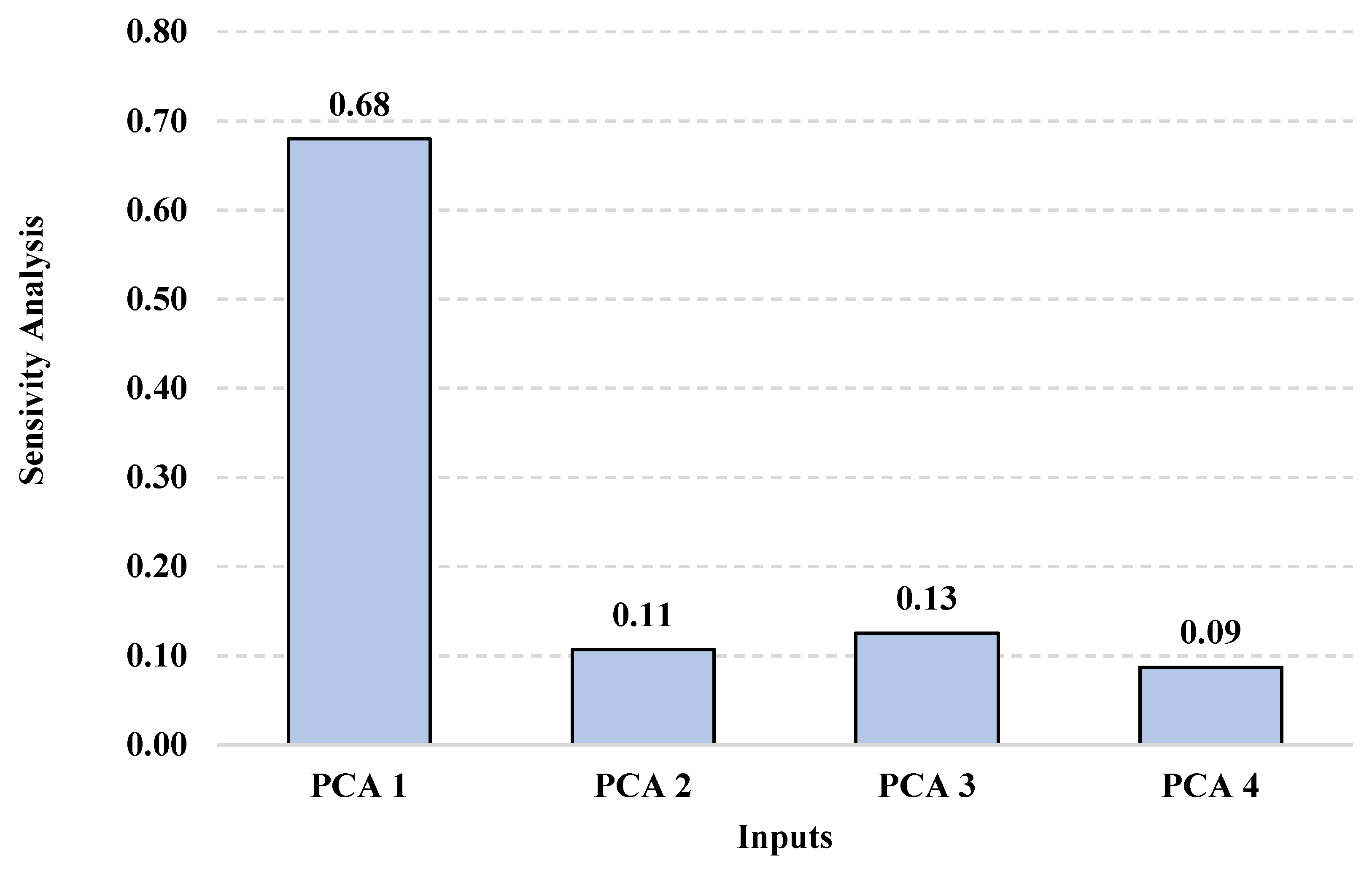
4. Sensitivity Analysis (SA)
5. Conclusions
- Increasing the number of inputs in the ANN increases the number of errors. PCA reduces the inputs, which improves the results in the combined PCA-ANN-based models for determining AR output.
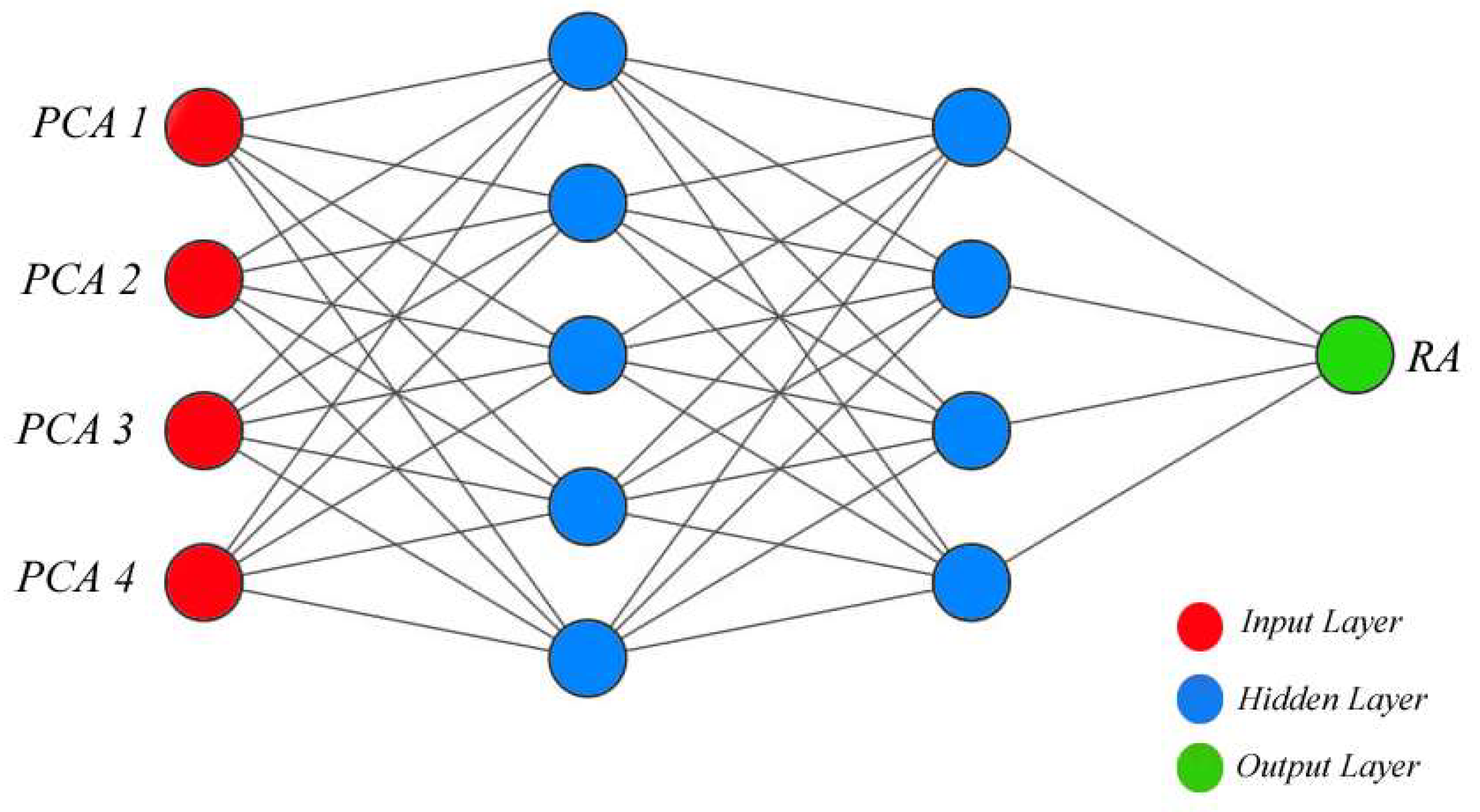
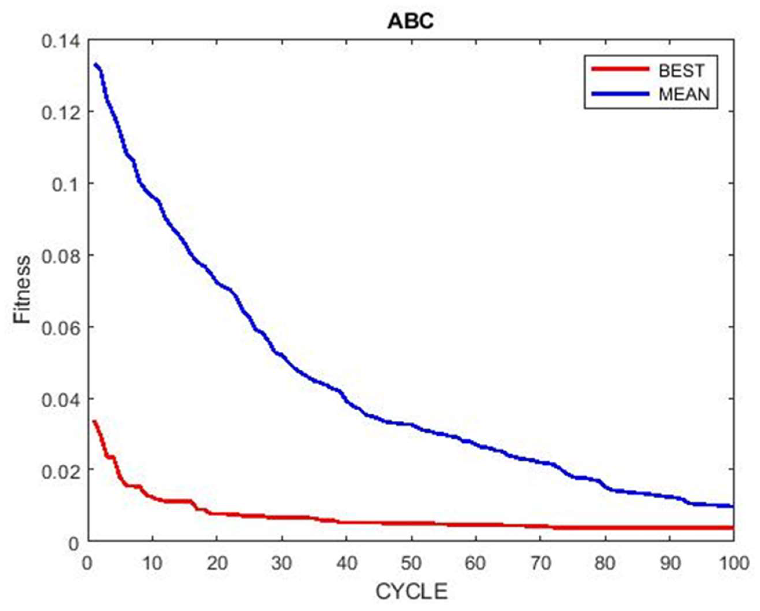
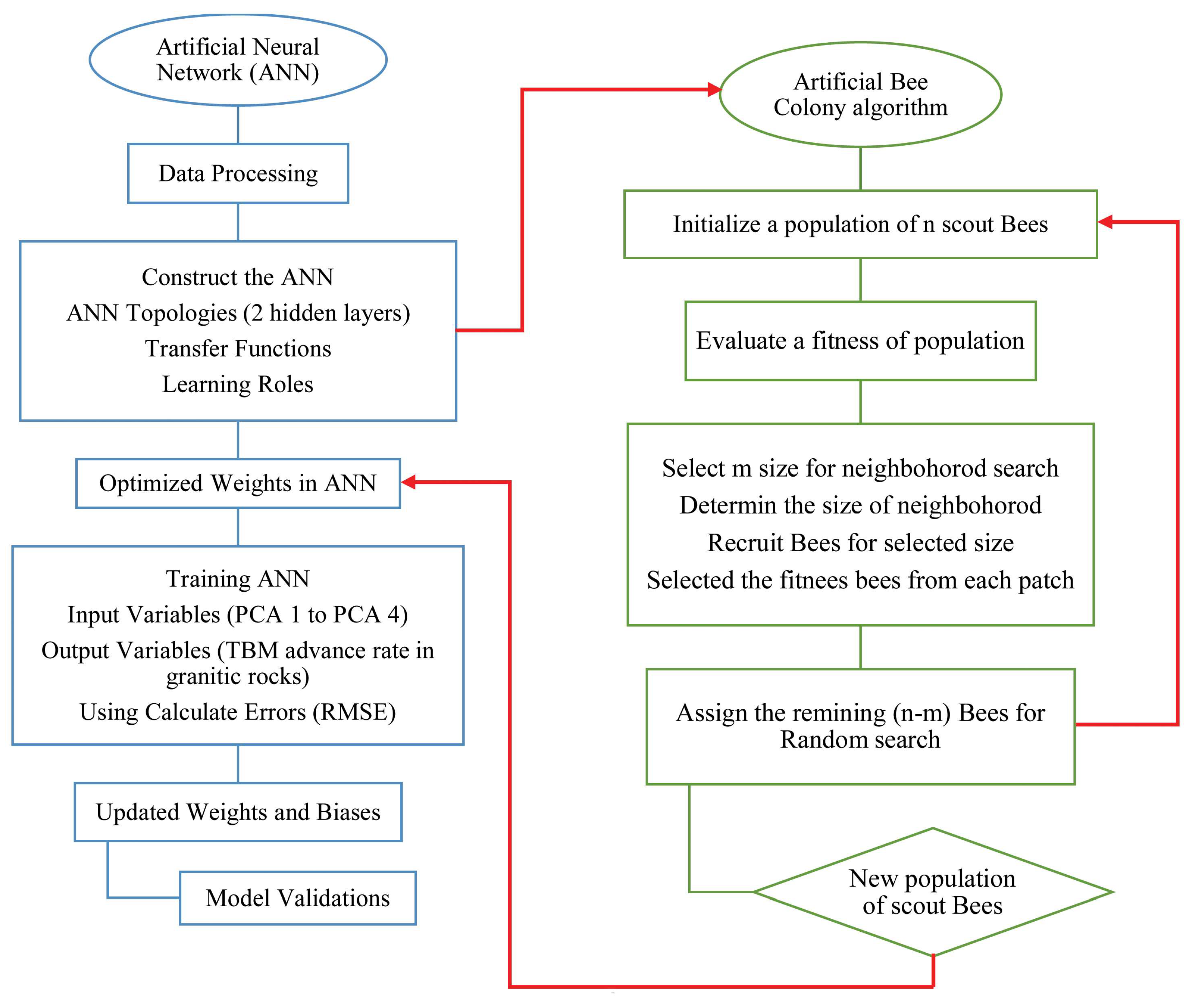
- After using the PCA results to reduce the ANN inputs, in order to optimize the weights of the ANN, the ABC algorithm was used to select the best structure for the ANNs and produce the least errors in the models. For this purpose, 20 models with different topologies were used, and the model with the 4-5-4-1 topology offered acceptable results.
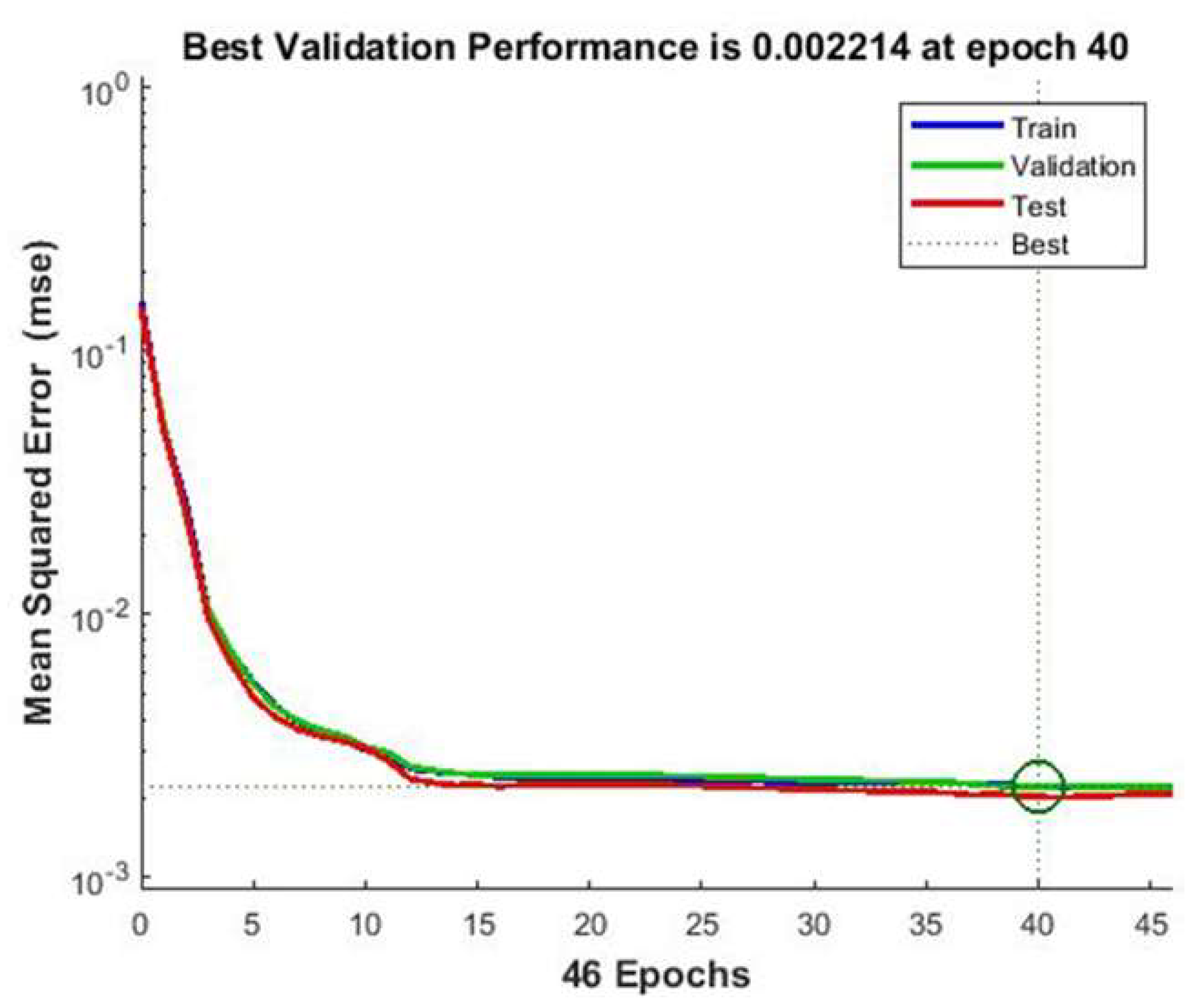
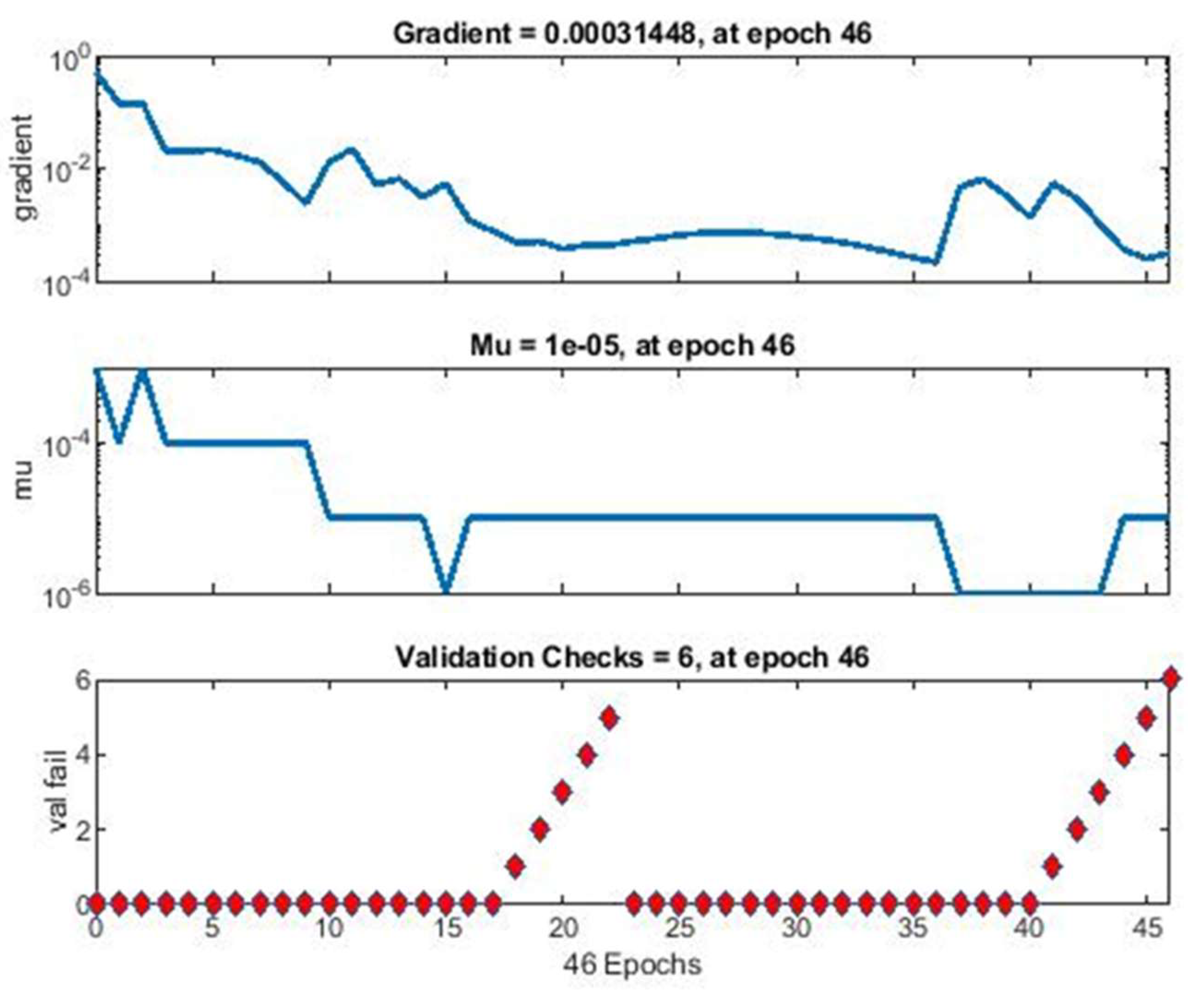
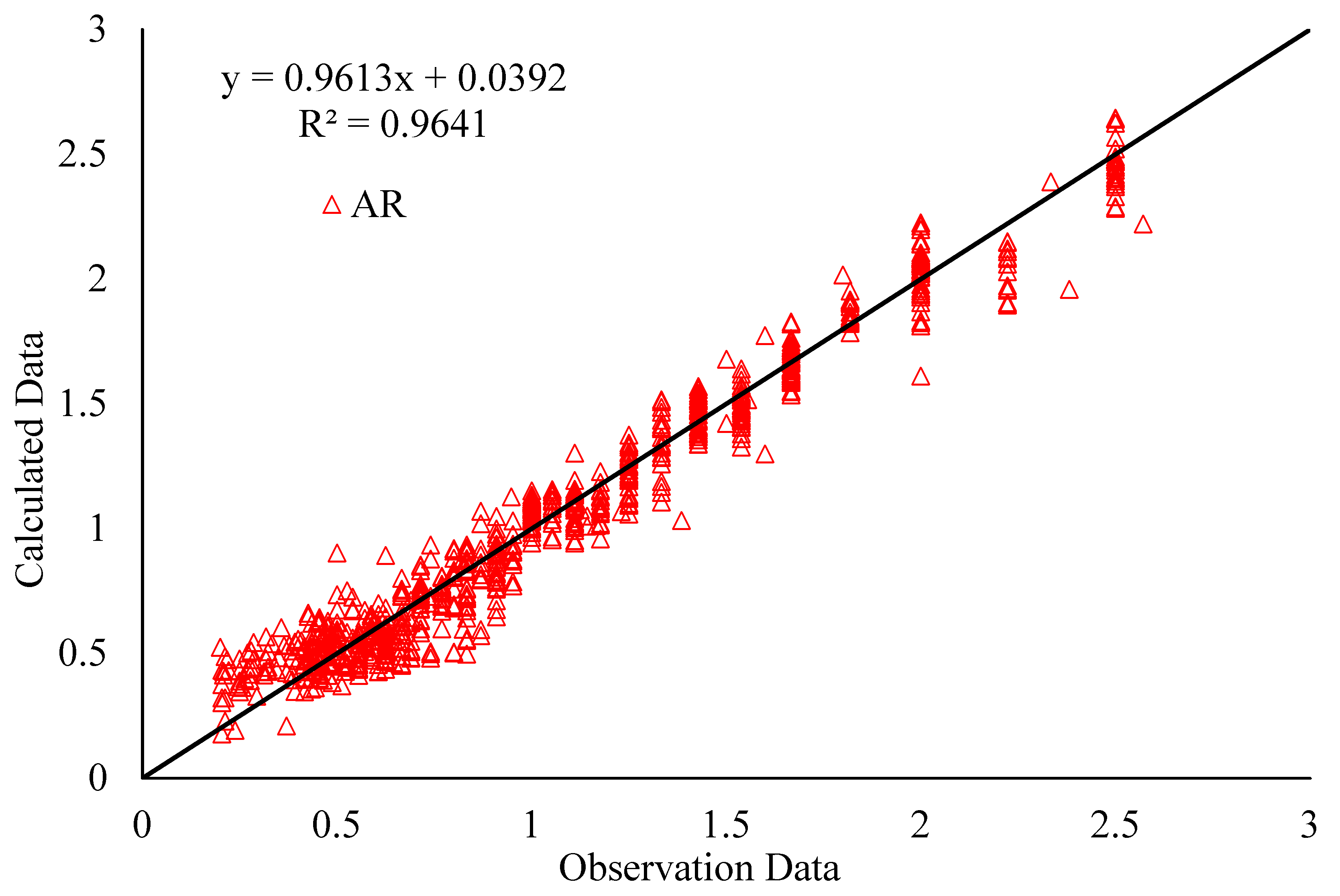
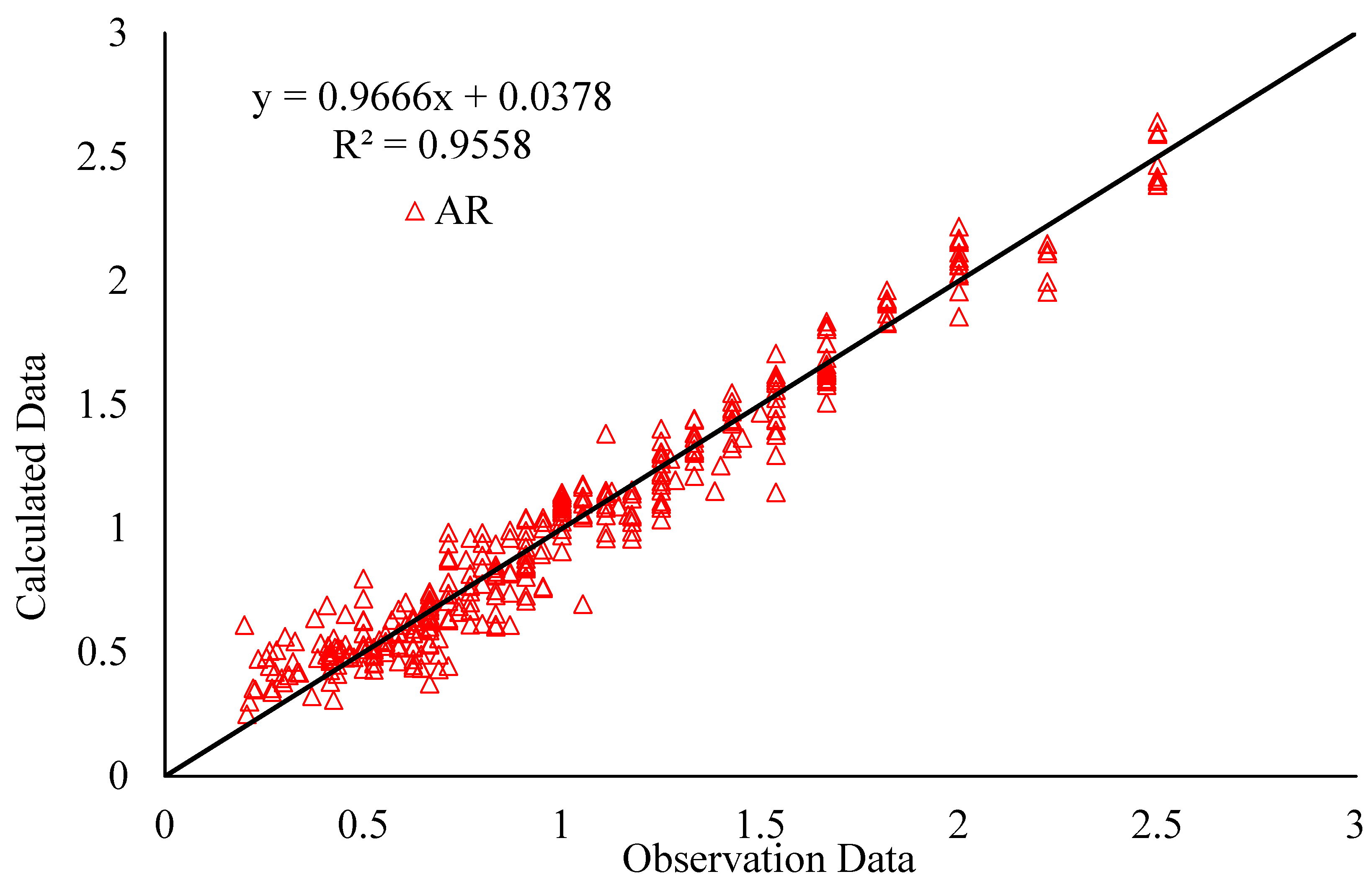
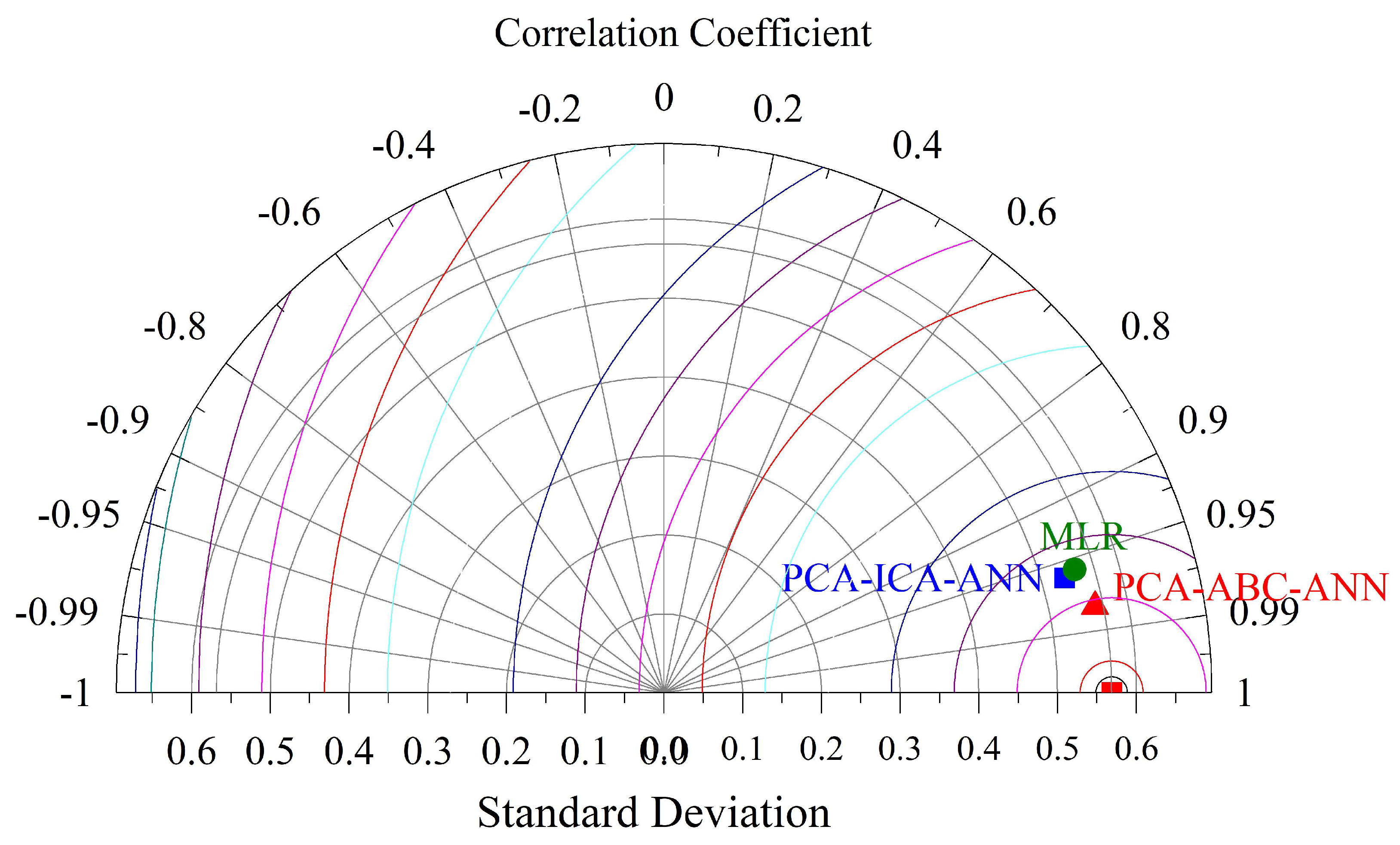
- The PCA-ABC-ANN model combined with the Levenberg–Marquardt learning algorithm and the hyperbolic tangent transfer function were more capable and accurate in predicting TBM AR values. In this model, the R2 values for TBM AR in the training and test stages were as 0.9641 and 0.9558, respectively, indicating the model’s high accuracy. On training data, RMSE, AAE, and VAF% of the PCA-ABC-ANN model for TBM AR values were 0.11, 0.12 and 96%, respectively, while in testing data, they were 0.12, 0.13, and 96%. The statistical indices of VAF, AAE, and RMSE presented in Table 7 indicate the model’s negligible error.
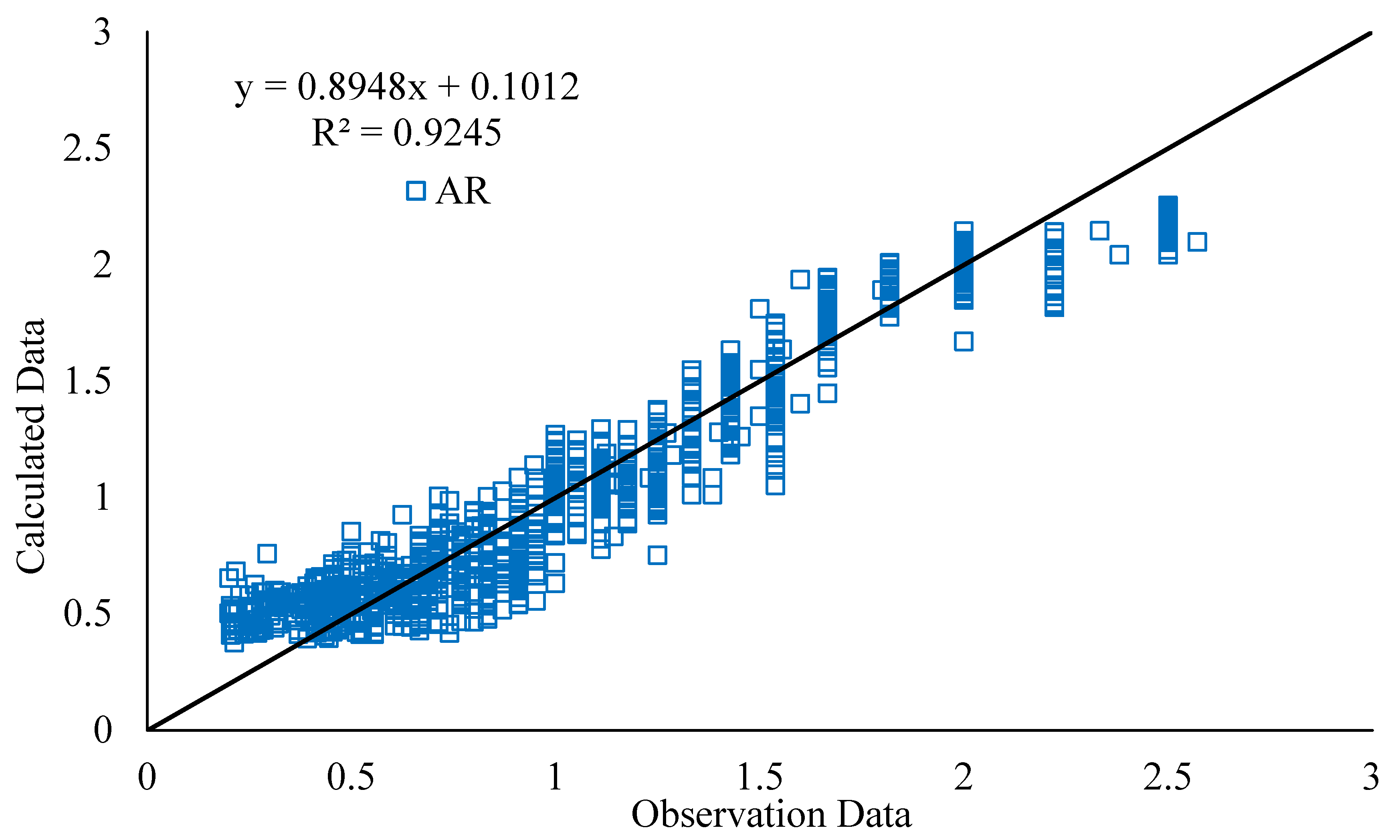
- To assess the accuracy of the ABC-optimized technique, it is compared with the ICA algorithm. For the PCA-ICA-ANN model on all data, RMSE, AAE, and VAF% for TBM AR values were 0.16, 0.17, and 92%, respectively.
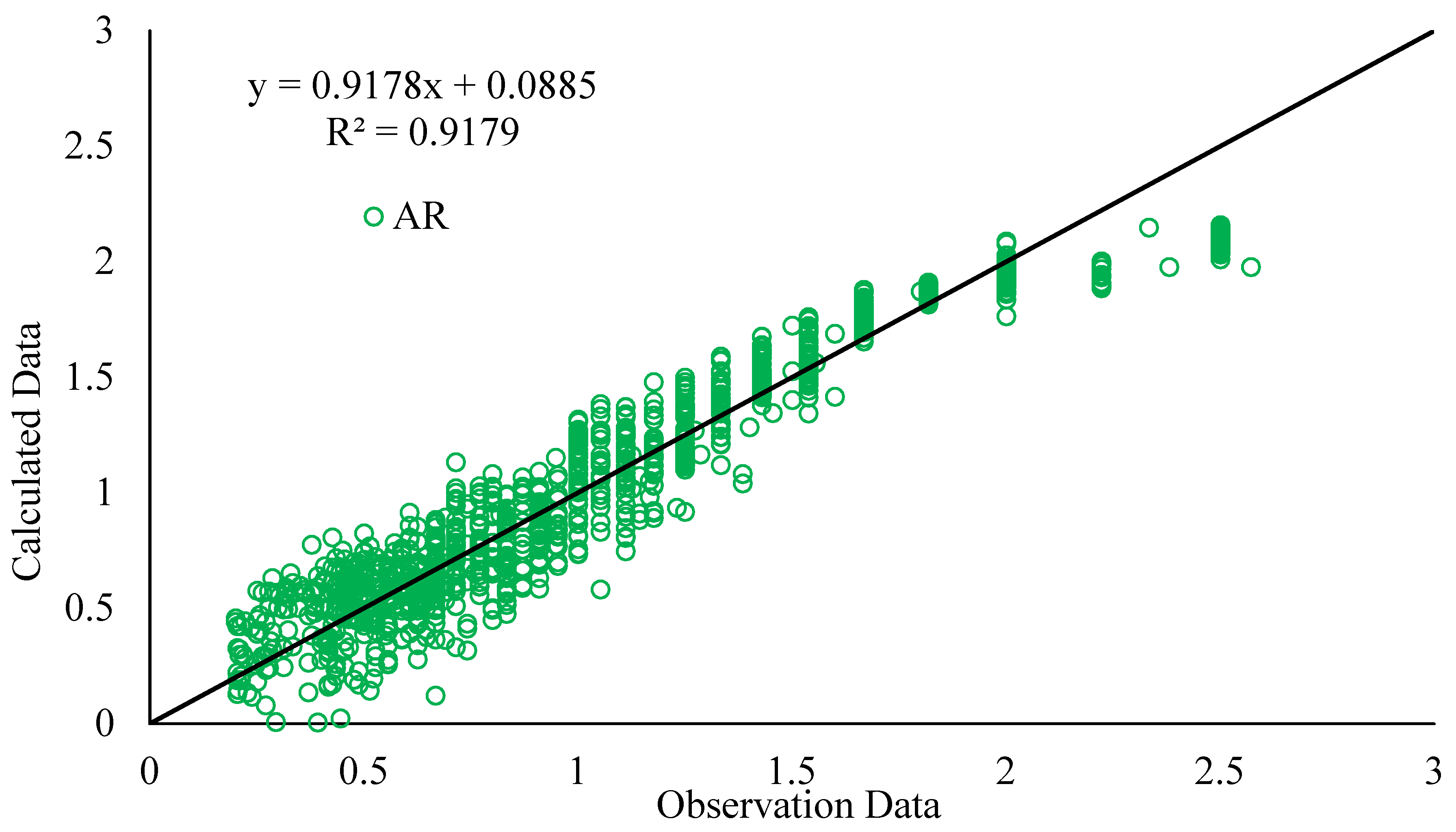
- The authors have used a statistical model with seven input variables. For the MLR model on all data, RMSE, AAE, and VAF% for TBM AR values were 0.16, 0.16, and 92%, respectively.
- According to the evaluation results, the ABC algorithm received a higher accuracy level than the ICA algorithm followed by the MLR model.
- The modeling procedure introduced in this study regarding reducing the number of inputs using PCA can be implemented in the other similar fields.
- The models in this study were developed for a granitic rock mass, which includes simple geological conditions. Therefore, these models should be used in very similar conditions if very close performance is needed. Of course, the error is higher if different geological conditions are examined.
Author Contributions
Funding
Institutional Review Board Statement
Informed Consent Statement
Data Availability Statement
Acknowledgments
Conflicts of Interest
References
- Armaghani, D.J.; Mohamad, E.T.; Narayanasamy, M.S.; Narita, N.; Yagiz, S. Development of hybrid intelligent models for predicting TBM penetration rate in hard rock condition. Tunn. Undergr. Space Technol. 2017, 63, 29–43. [Google Scholar] [CrossRef]
- Zhou, J.; Yazdani Bejarbaneh, B.; Jahed Armaghani, D.; Tahir, M.M. Forecasting of TBM advance rate in hard rock condition based on artificial neural network and genetic programming techniques. Bull. Eng. Geol. Environ. 2020, 79, 2069–2084. [Google Scholar] [CrossRef]
- Farmer, I.W.; Glossop, N.H. Mechanics of disc cutter penetration. Tunn. Tunn. 1980, 12, 22–25. [Google Scholar]
- Snowdon, R.A.; Ryley, M.D.; Temporal, J. A study of disc cutting in selected British rocks. Int. J. Rock Mech. Min. Sci. Geomech. Abstracts 1982, 19, 107–121. [Google Scholar] [CrossRef]
- Sanio, H.P. Prediction of the performance of disc cutters in anisotropic rock. Int. J. Rock Mech. Min. Sci. Geomech. Abstracts 1985, 22, 153–161. [Google Scholar] [CrossRef]
- Rostami, J.; Ozdemir, L. A new model for performance prediction of hard rock TBMs. In Proceedings of the 1993 Rapid Excavation and Tunneling Conference, Boston, MA, USA, 13–17 June 1993; Society for Mining, Metallogy & Exploration, Inc.: Englewood, CO, USA, 1993; p. 793. [Google Scholar]
- Yagiz, S. Development of Rock Fracture and Brittleness Indices to Quantify the Effects of Rock Mass Features and Toughness in the CSM Model Basic Penetration for Hard Rock Tunneling Machines; Colorado School of Mines: Golden, CO, USA, 2002. [Google Scholar]
- Yang, H.; Wang, H.; Zhou, X. Analysis on the rock–cutter interaction mechanism during the TBM tunneling process. Rock Mech. Rock Eng. 2016, 49, 1073–1090. [Google Scholar] [CrossRef]
- Armaghani, D.J.; Faradonbeh, R.S.; Momeni, E.; Fahimifar, A.; Tahir, M.M. Performance prediction of tunnel boring machine through developing a gene expression programming equation. Eng. Comput. 2018, 34, 129–141. [Google Scholar] [CrossRef]
- Zhou, J.; Qiu, Y.; Zhu, S.; Armaghani, D.J.; Li, C.; Nguyen, H.; Yagiz, S. Optimization of support vector machine through the use of metaheuristic algorithms in forecasting TBM advance rate. Eng. Appl. Artif. Intell. 2021, 97, 104015. [Google Scholar] [CrossRef]
- Yang, H.; Liu, J.; Liu, B. Investigation on the cracking character of jointed rock mass beneath TBM disc cutter. Rock Mech. Rock Eng. 2018, 51, 1263–1277. [Google Scholar] [CrossRef]
- Grima, M.A.; Bruines, P.A.; Verhoef, P.N.W. Modeling tunnel boring machine performance by neuro-fuzzy methods. Tunn. Undergr. Space Technol. 2000, 15, 259–269. [Google Scholar] [CrossRef]
- Yagiz, S.; Gokceoglu, C.; Sezer, E.; Iplikci, S. Application of two non-linear prediction tools to the estimation of tunnel boring machine performance. Eng. Appl. Artif. Intell. 2009, 22, 808–814. [Google Scholar] [CrossRef]
- Armaghani, D.J.; Koopialipoor, M.; Marto, A.; Yagiz, S. Application of several optimization techniques for estimating TBM advance rate in granitic rocks. J. Rock Mech. Geotech. Eng. 2019, 11, 779–789. [Google Scholar] [CrossRef]
- Mahdevari, S.; Shahriar, K.; Yagiz, S.; Shirazi, M.A. A support vector regression model for predicting tunnel boring machine penetration rates. Int. J. Rock Mech. Min. Sci. 2014, 72, 214–229. [Google Scholar] [CrossRef]
- Oraee, K.; Khorami, M.T.; Hosseini, N. Prediction of the penetration rate of TBM using adaptive neuro fuzzy inference system (ANFIS). In Proceedings of the 2012 SME Annual Meeting & Exhibit 2012 (SME 2012): From Mine to Market, Seattle, WA, USA, 19–22 February 2012; pp. 297–302. [Google Scholar]
- Jahed Armaghani, D.; Azizi, A. Applications of Artificial Intelligence in Tunnelling and Underground Space Technology; Springer Nature: Singapore, 2021; ISBN 9811610347. [Google Scholar] [CrossRef]
- Yagiz, S. New equations for predicting the field penetration index of tunnel boring machines in fractured rock mass. Arab. J. Geosci. 2017, 10, 33. [Google Scholar] [CrossRef]
- Delisio, A.; Zhao, J.; Einstein, H.H. Analysis and prediction of TBM performance in blocky rock conditions at the Lötschberg Base Tunnel. Tunn. Undergr. Space Technol. 2013, 33, 131–142. [Google Scholar] [CrossRef]
- Farrokh, E.; Rostami, J.; Laughton, C. Study of various models for estimation of penetration rate of hard rock TBMs. Tunn. Undergr. Space Technol. 2012, 30, 110–123. [Google Scholar] [CrossRef]
- Grima, M.A.; Verhoef, P.N.W. Forecasting rock trencher performance using fuzzy logic. Int. J. Rock Mech. Min. Sci. 1999, 36, 413–432. [Google Scholar]
- Salimi, A.; Esmaeili, M. Utilising of linear and non-linear prediction tools for evaluation of penetration rate of tunnel boring machine in hard rock condition. Int. J. Min. Miner. Eng. 2013, 4, 249–264. [Google Scholar] [CrossRef]
- Salimi, A.; Faradonbeh, R.S.; Monjezi, M.; Moormann, C. TBM performance estimation using a classification and regression tree (CART) technique. Bull. Eng. Geol. Environ. 2018, 77, 429–440. [Google Scholar] [CrossRef]
- Ghasemi, E.; Yagiz, S.; Ataei, M. Predicting penetration rate of hard rock tunnel boring machine using fuzzy logic. Bull. Eng. Geol. Environ. 2014, 73, 23–35. [Google Scholar] [CrossRef]
- Simoes, M.G.; Kim, T. Fuzzy modeling approaches for the prediction of machine utilization in hard rock tunnel boring machines. In Proceedings of the Conference Record of the 2006 IEEE Industry Applications Conference Forty-First IAS Annual Meeting, Tampa, FL, USA, 8–12 October 2006; Volume 2, pp. 947–954. [Google Scholar]
- Benardos, A.G.; Kaliampakos, D.C. Modelling TBM performance with artificial neural networks. Tunn. Undergr. Space Technol. 2004, 19, 597–605. [Google Scholar] [CrossRef]
- Feng, S.; Chen, Z.; Luo, H.; Wang, S.; Zhao, Y.; Liu, L.; Ling, D.; Jing, L. Tunnel boring machines (TBM) performance prediction: A case study using big data and deep learning. Tunn. Undergr. Space Technol. 2021, 110, 103636. [Google Scholar] [CrossRef]
- Adoko, A.C.; Yagiz, S. Fuzzy inference system-based for TBM field penetration index estimation in rock mass. Geotech. Geol. Eng. 2019, 37, 1533–1553. [Google Scholar] [CrossRef]
- Salimi, A.; Rostami, J.; Moormann, C.; Delisio, A. Application of non-linear regression analysis and artificial intelligence algorithms for performance prediction of hard rock TBMs. Tunn. Undergr. Space Technol. 2016, 58, 236–246. [Google Scholar] [CrossRef]
- Koopialipoor, M.; Nikouei, S.S.; Marto, A.; Fahimifar, A.; Armaghani, D.J.; Mohamad, E.T. Predicting tunnel boring machine performance through a new model based on the group method of data handling. Bull. Eng. Geol. Environ. 2018, 78, 3799–3813. [Google Scholar] [CrossRef]
- Minh, V.T.; Katushin, D.; Antonov, M.; Veinthal, R. Regression Models and Fuzzy Logic Prediction of TBM Penetration Rate. Open Eng. 2017, 7, 60–68. [Google Scholar] [CrossRef]
- Zhou, J.; Qiu, Y.; Armaghani, D.J.; Zhang, W.; Li, C.; Zhu, S.; Tarinejad, R. Predicting TBM penetration rate in hard rock condition: A comparative study among six XGB-based metaheuristic techniques. Geosci. Front. 2020, 12, 101091. [Google Scholar] [CrossRef]
- Zeng, J.; Roy, B.; Kumar, D.; Mohammed, A.S.; Armaghani, D.J.; Zhou, J.; Mohamad, E.T. Proposing several hybrid PSO-extreme learning machine techniques to predict TBM performance. In Engineering with Computers; Springer: Berlin/Heidelberg, Germany, 2021. [Google Scholar] [CrossRef]
- Hajihassani, M.; Abdullah, S.S.; Asteris, P.G.; Armaghani, D.J. A Gene Expression Programming Model for Predicting Tunnel Convergence. Appl. Sci. 2019, 9, 4650. [Google Scholar] [CrossRef] [Green Version]
- Asteris, P.G.; Armaghani, D.J.; Hatzigeorgiou, G.D.; Karayannis, C.G.; Pilakoutas, K. Predicting the shear strength of reinforced concrete beams using Artificial Neural Networks. Comput. Concr. 2019, 24, 469–488. [Google Scholar]
- Apostolopoulou, M.; Armaghani, D.J.; Bakolas, A.; Douvika, M.G.; Moropoulou, A.; Asteris, P.G. Compressive strength of natural hydraulic lime mortars using soft computing techniques. Procedia Struct. Integr. 2019, 17, 914–923. [Google Scholar] [CrossRef]
- Armaghani, D.J.; Hatzigeorgiou, G.D.; Karamani, C.; Skentou, A.; Zoumpoulaki, I.; Asteris, P.G. Soft computing-based techniques for concrete beams shear strength. Procedia Struct. Integr. 2019, 17, 924–933. [Google Scholar] [CrossRef]
- Yang, H.Q.; Xing, S.G.; Wang, Q.; Li, Z. Model test on the entrainment phenomenon and energy conversion mechanism of flow-like landslides. Eng. Geol. 2018, 239, 119–125. [Google Scholar] [CrossRef]
- Yang, H.Q.; Lan, Y.F.; Lu, L.; Zhou, X.P. A quasi-three-dimensional spring-deformable-block model for runout analysis of rapid landslide motion. Eng. Geol. 2015, 185, 20–32. [Google Scholar] [CrossRef]
- Jian, Z.; Shi, X.; Huang, R.; Qiu, X.; Chong, C. Feasibility of stochastic gradient boosting approach for predicting rockburst damage in burst-prone mines. Trans. Nonferrous Met. Soc. China 2016, 26, 1938–1945. [Google Scholar]
- Zhou, J.; Li, E.; Yang, S.; Wang, M.; Shi, X.; Yao, S.; Mitri, H.S. Slope stability prediction for circular mode failure using gradient boosting machine approach based on an updated database of case histories. Saf. Sci. 2019, 118, 505–518. [Google Scholar] [CrossRef]
- Kardani, N.; Bardhan, A.; Samui, P.; Nazem, M.; Zhou, A.; Armaghani, D.J. A novel technique based on the improved firefly algorithm coupled with extreme learning machine (ELM-IFF) for predicting the thermal conductivity of soil. In Engineering with Computers; Springer: Berlin/Heidelberg, Germany, 2021. [Google Scholar] [CrossRef]
- Zeng, J.; Asteris, P.G.; Mamou, A.P.; Mohammed, A.S.; Golias, E.A.; Armaghani, D.J.; Faizi, K.; Hasanipanah, M. The Effectiveness of Ensemble-Neural Network Techniques to Predict Peak Uplift Resistance of Buried Pipes in Reinforced Sand. Appl. Sci. 2021, 11, 908. [Google Scholar] [CrossRef]
- Momeni, E.; Yarivand, A.; Dowlatshahi, M.B.; Armaghani, D.J. An Efficient Optimal Neural Network Based on Gravitational Search Algorithm in Predicting the Deformation of Geogrid-Reinforced Soil Structures. Transp. Geotech. 2020, 26, 100446. [Google Scholar] [CrossRef]
- Hasanipanah, M.; Monjezi, M.; Shahnazar, A.; Armaghani, D.J.; Farazmand, A. Feasibility of indirect determination of blast induced ground vibration based on support vector machine. Measurement 2015, 75, 289–297. [Google Scholar] [CrossRef]
- Asteris, P.G.; Rizal, F.I.M.; Koopialipoor, M.; Roussis, P.C.; Ferentinou, M.; Armaghani, D.J.; Gordan, B. Slope Stability Classification under Seismic Conditions Using Several Tree-Based Intelligent Techniques. Appl. Sci. 2022, 12, 1753. [Google Scholar] [CrossRef]
- Asteris, P.G.; Lourenço, P.B.; Roussis, P.C.; Adami, C.E.; Armaghani, D.J.; Cavaleri, L.; Chalioris, C.E.; Hajihassani, M.; Lemonis, M.E.; Mohammed, A.S. Revealing the nature of metakaolin-based concrete materials using artificial intelligence techniques. Constr. Build. Mater. 2022, 322, 126500. [Google Scholar] [CrossRef]
- Armaghani, D.J.; Mamou, A.; Maraveas, C.; Roussis, P.C.; Siorikis, V.G.; Skentou, A.D.; Asteris, P.G. Predicting the unconfined compressive strength of granite using only two non-destructive test indexes. Geomech. Eng. 2021, 25, 317–330. [Google Scholar]
- Parsajoo, M.; Armaghani, D.J.; Mohammed, A.S.; Khari, M.; Jahandari, S. Tensile strength prediction of rock material using non-destructive tests: A comparative intelligent study. Transp. Geotech. 2021, 31, 100652. [Google Scholar] [CrossRef]
- Asteris, P.G.; Mamou, A.; Hajihassani, M.; Hasanipanah, M.; Koopialipoor, M.; Le, T.-T.; Kardani, N.; Armaghani, D.J. Soft computing based closed form equations correlating L and N-type Schmidt hammer rebound numbers of rocks. Transp. Geotech. 2021, 29, 100588. [Google Scholar] [CrossRef]
- Plevris, V.; Asteris, P.G. Modeling of masonry failure surface under biaxial compressive stress using Neural Networks. Constr. Build. Mater. 2014, 55, 447–461. [Google Scholar] [CrossRef]
- Liao, J.; Asteris, P.G.; Cavaleri, L.; Mohammed, A.S.; Lemonis, M.E.; Tsoukalas, M.Z.; Skentou, A.D.; Maraveas, C.; Koopialipoor, M.; Armaghani, D.J. Novel Fuzzy-Based Optimization Approaches for the Prediction of Ultimate Axial Load of Circular Concrete-Filled Steel Tubes. Buildings 2021, 11, 629. [Google Scholar] [CrossRef]
- Barkhordari, M.S.; Armaghani, D.J.; Mohammed, A.S.; Ulrikh, D.V. Data-Driven Compressive Strength Prediction of Fly Ash Concrete Using Ensemble Learner Algorithms. Buildings 2022, 12, 132. [Google Scholar] [CrossRef]
- Lee, Y.; Oh, S.-H.; Kim, M.W. The effect of initial weights on premature saturation in back-propagation learning. In Proceedings of the IJCNN-91-Seattle International Joint Conference on Neural Networks, Seattle, WA, USA, 8–12 July 1991; Volume 1, pp. 765–770. [Google Scholar]
- Wang, X.; Tang, Z.; Tamura, H.; Ishii, M.; Sun, W.D. An improved backpropagation algorithm to avoid the local minima problem. Neurocomputing 2004, 56, 455–460. [Google Scholar] [CrossRef]
- Alavi Nezhad Khalil Abad, S.V.; Yilmaz, M.; Jahed Armaghani, D.; Tugrul, A. Prediction of the durability of limestone aggregates using computational techniques. Neural Comput. Appl. 2016, 29, 423–433. [Google Scholar] [CrossRef]
- Koopialipoor, M.; Jahed Armaghani, D.; Haghighi, M.; Ghaleini, E.N. A neuro-genetic predictive model to approximate overbreak induced by drilling and blasting operation in tunnels. Bull. Eng. Geol. Environ. 2019, 78, 981–990. [Google Scholar] [CrossRef]
- Nikoo, M.; Hadzima-Nyarko, M.; Karlo Nyarko, E.; Nikoo, M. Determining the natural frequency of cantilever beams using ANN and heuristic search. Appl. Artif. Intell. 2018, 32, 309–334. [Google Scholar] [CrossRef]
- Bishop, C.M. Neural Networks for Pattern Recognition; Oxford University Press: Oxford, UK, 1995; ISBN 0198538642. [Google Scholar]
- Haykin, S. Neural Networks and Learning Machines, 3rd ed.; Pearson Prentice Hall: Hoboken, NJ, USA, 2009. [Google Scholar]
- Murlidhar, B.R.; Armaghani, D.J.; Mohamad, E.T. Intelligence Prediction of Some Selected Environmental Issues of Blasting: A Review. Open Constr. Build. Technol. J. 2020, 14, 298–308. [Google Scholar] [CrossRef]
- Mohamad, E.T.; Noorani, S.A.; Armaghani, D.J.; Saad, R. Simulation of blasting induced ground vibration by using artificial neural network. Electron. J. Geotech. Eng. 2012, 17, 2571–2584. [Google Scholar]
- Tereshko, V. Reaction-diffusion model of a honeybee colony’s foraging behaviour. In Proceedings of the International Conference on Parallel Problem Solving from Nature; Springer: Berlin/Heidelberg, Germany, 2000; pp. 807–816. [Google Scholar]
- Asteris, P.G.; Nikoo, M. Artificial bee colony-based neural network for the prediction of the fundamental period of infilled frame structures. Neural Comput. Appl. 2019, 31, 4837–4847. [Google Scholar] [CrossRef]
- Karaboga, D.; Akay, B. A comparative study of artificial bee colony algorithm. Appl. Math. Comput. 2009, 214, 108–132. [Google Scholar] [CrossRef]
- Zhou, J.; Koopialipoor, M.; Li, E.; Armaghani, D.J. Prediction of rockburst risk in underground projects developing a neuro-bee intelligent system. Bull. Eng. Geol. Environ. 2020, 79, 4265–4279. [Google Scholar] [CrossRef]
- Le, L.T.; Nguyen, H.; Dou, J.; Zhou, J. A comparative study of PSO-ANN, GA-ANN, ICA-ANN, and ABC-ANN in estimating the heating load of buildings’ energy efficiency for smart city planning. Appl. Sci. 2019, 9, 2630. [Google Scholar] [CrossRef] [Green Version]
- Jolliffe, I.T. Principal components in regression analysis. In Principal Component Analysis; Springer: New York, NY, USA, 1986; pp. 129–155. [Google Scholar] [CrossRef]
- Sadowski, Ł.; Nikoo, M.; Nikoo, M. Principal component analysis combined with a self organization feature map to determine the pull-off adhesion between concrete layers. Constr. Build. Mater. 2015, 78, 386–396. [Google Scholar] [CrossRef]
- Ulusay, R.; Hudson, J.A. The complete ISRM suggested methods for rock characterization, testing and monitoring: 1974–2006. In International Society for Rock Mechanics, Commission on Testing Methods; ISRM Turkish Natl. Group: Ankara, Turkey, 2007; Volume 628. [Google Scholar]
- Madar, V. Direct formulation to Cholesky decomposition of a general nonsingular correlation matrix. Stat. Probab. Lett. 2015, 103, 142–147. [Google Scholar] [CrossRef] [PubMed] [Green Version]
- Jiang, B. Covariance selection by thresholding the sample correlation matrix. Stat. Probab. Lett. 2013, 83, 2492–2498. [Google Scholar] [CrossRef]
- Harandizadeh, H.; Armaghani, D.J. Prediction of air-overpressure induced by blasting using an ANFIS-PNN model optimized by GA. Appl. Soft Comput. 2020, 99, 106904. [Google Scholar] [CrossRef]
- Harandizadeh, H.; Armaghani, D.J.; Mohamad, E.T. Development of fuzzy-GMDH model optimized by GSA to predict rock tensile strength based on experimental datasets. Neural Comput. Appl. 2020, 32, 14047–14067. [Google Scholar] [CrossRef]
- Harandizadeh, H.; Armaghani, D.J.; Khari, M. A new development of ANFIS–GMDH optimized by PSO to predict pile bearing capacity based on experimental datasets. Eng. Comput. 2021, 37, 685–700. [Google Scholar] [CrossRef]
- Armaghani, D.J.; Harandizadeh, H.; Momeni, E. Load carrying capacity assessment of thin-walled foundations: An ANFIS–PNN model optimized by genetic algorithm. In Engineering with Computers; Springer: Berlin/Heidelberg, Germany, 2021. [Google Scholar] [CrossRef]
- Bowden, G.J.; Dandy, G.C.; Maier, H.R. Input determination for neural network models in water resources applications. Part 1—background and methodology. J. Hydrol. 2005, 301, 75–92. [Google Scholar] [CrossRef]
- Li, J.; Heap, A.D. A Review of Spatial Interpolation Methods for Environmental Scientists; Australian Gvernment: Canberra, Australia, 2008; ISBN 9781921498305. [Google Scholar]
- Nikoo, M.; Torabian Moghadam, F.; Sadowski, Ł. Prediction of concrete compressive strength by evolutionary artificial neural networks. Adv. Mater. Sci. Eng. 2015, 2015, 849126. [Google Scholar] [CrossRef]
- Mohamad, E.T.; Armaghani, D.J.; Mahdyar, A.; Komoo, I.; Kassim, K.A.; Abdullah, A.; Majid, M.Z.A. Utilizing regression models to find functions for determining ripping production based on laboratory tests. Measurement 2017, 111, 216–225. [Google Scholar] [CrossRef]
- Gordan, B.; Armaghani, D.J.; Adnan, A.B.; Rashid, A.S.A. A New Model for Determining Slope Stability Based on Seismic Motion Performance. Soil Mech. Found. Eng. 2016, 53, 344–351. [Google Scholar] [CrossRef]
- Atashpaz-Gargari, E.; Lucas, C. Imperialist competitive algorithm: An algorithm for optimization inspired by imperialistic competition. In Proceedings of the 2007 IEEE Congress on Evolutionary Computation, Singapore, 25–28 September 2007; pp. 4661–4667. [Google Scholar]
- Sadowski, L.; Nikoo, M. Corrosion current density prediction in reinforced concrete by imperialist competitive algorithm. Neural Comput. Appl. 2014, 25, 1627–1638. [Google Scholar] [CrossRef] [PubMed] [Green Version]
- Armaghani, D.J.; Hasanipanah, M.; Amnieh, H.B.; Mohamad, E.T. Feasibility of ICA in approximating ground vibration resulting from mine blasting. Neural Comput. Appl. 2018, 29, 457–465. [Google Scholar] [CrossRef]
- Armaghani, D.J.; Hasanipanah, M.; Mohamad, E.T. A combination of the ICA-ANN model to predict air-overpressure resulting from blasting. Eng. Comput. 2016, 32, 155–171. [Google Scholar] [CrossRef]
- Marto, A.; Hajihassani, M.; Jahed Armaghani, D.; Tonnizam Mohamad, E.; Makhtar, A.M. A novel approach for blast-induced flyrock prediction based on imperialist competitive algorithm and artificial neural network. Sci. World J. 2014, 2014, 643715. [Google Scholar] [CrossRef]
- Lek, S.; Delacoste, M.; Baran, P.; Dimopoulos, I.; Lauga, J.; Aulagnier, S. Application of neural networks to modelling nonlinear relationships in ecology. Ecol. Modell. 1996, 90, 39–52. [Google Scholar] [CrossRef]
- Gevrey, M.; Dimopoulos, I.; Lek, S. Review and comparison of methods to study the contribution of variables in artificial neural network models. Ecol. Model. 2003, 160, 249–264. [Google Scholar] [CrossRef]
- Jahed Armaghani, D.; Azizi, A. Armaghani, D.; Azizi, A. A Comparative Study of Artificial Intelligence Techniques to Estimate TBM Performance in Various Weathering Zones. In Applications of Artificial Intelligence in Tunnelling and Underground Space Technology; Springer: Singapore, 2021; pp. 55–70. [Google Scholar] [CrossRef]
- Jahed Armaghani, D.; Azizi, A. Empirical, Statistical, and Intelligent Techniques for TBM Performance Prediction. In Applications of Artificial Intelligence in Tunnelling and Underground Space Technology; Springer: Singapore, 2021; pp. 17–32. [Google Scholar] [CrossRef]
- Yang, H.; Wang, Z.; Song, K. A new hybrid grey wolf optimizer-feature weighted-multiple kernel-support vector regression technique to predict TBM performance. In Engineering with Computers; Springer: Berlin/Heidelberg, Germany, 2022; Volume 38, pp. 2469–2482. [Google Scholar] [CrossRef]


| Factor | Unit | Type | Max | Min | Average | STD |
|---|---|---|---|---|---|---|
| RQD | % | Input | 95 | 10 | 53.79 | 27.85 |
| UCS | MPa | Input | 193 | 45.4 | 134.68 | 44.30 |
| RMR | - | Input | 95 | 46 | 72.74 | 15.71 |
| BTS | MPa | Input | 15.68 | 4.69 | 10.26 | 4.04 |
| WZ | - | Input | 3 | 1 | 1.68 | 0.69 |
| TFPC | kN | Input | 497.67 | 91.34 | 303.26 | 77.76 |
| RPM | rev/min | Input | 11.95 | 4.54 | 8.91 | 2.26 |
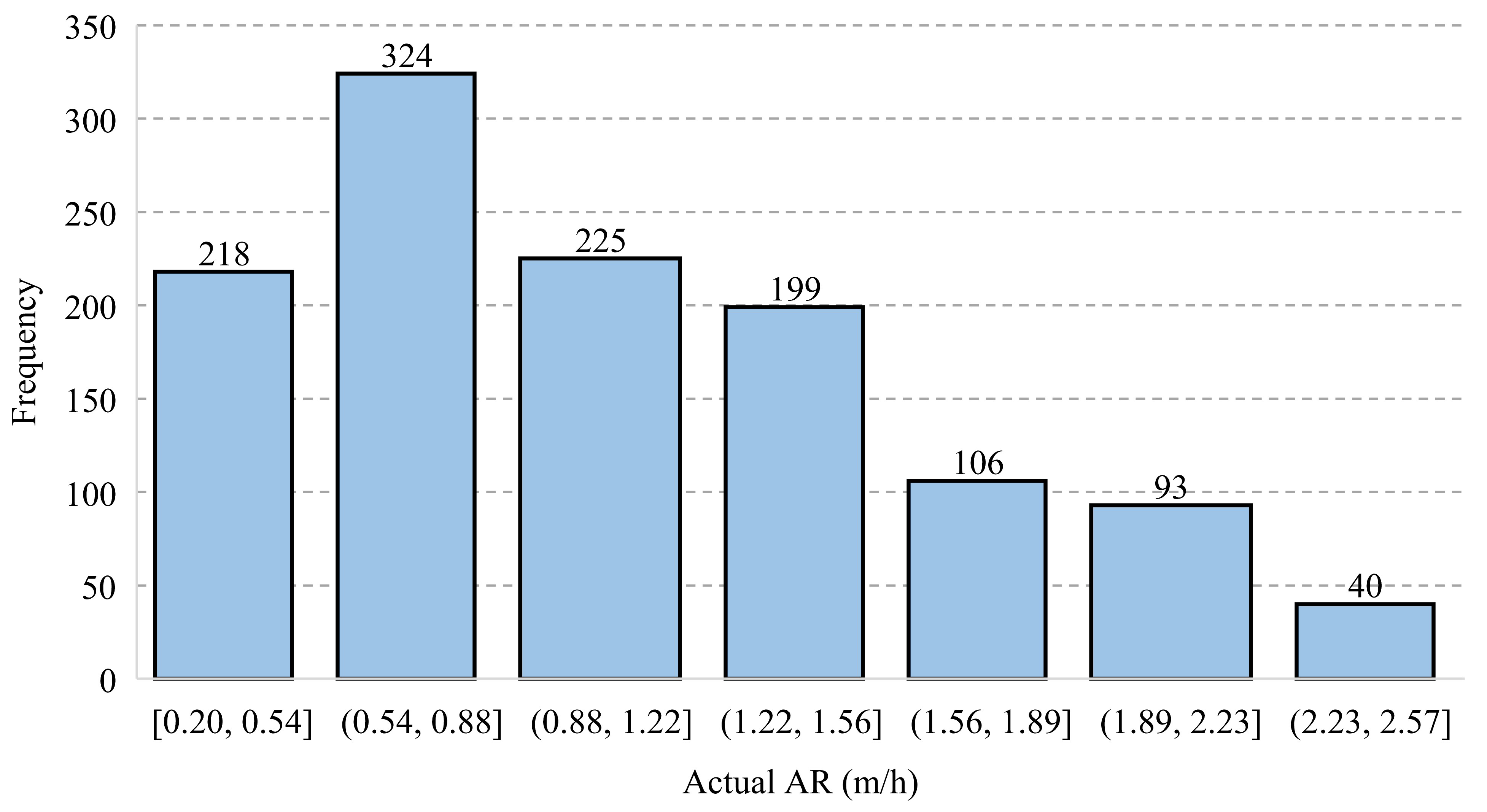
| TBM AR | m/h | Output | 2.57 | 0.20 | 1.08 | 0.57 |
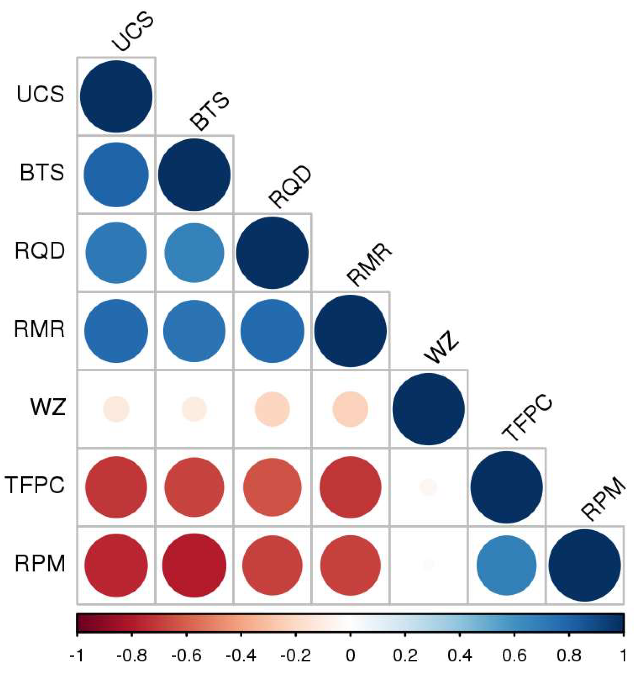
| Name | UCS | BTS | RQD | RMR | WZ | TFPC | RPM |
|---|---|---|---|---|---|---|---|
| UCS | 1 | ||||||
| BTS | 0.8 | 1 | |||||
| RQD | 0.71 | 0.67 | 1 | ||||
| RMR | 0.77 | 0.73 | 0.77 | 1 | |||
| WZ | −0.12 | −0.11 | −0.22 | −0.23 | 1 | ||
| TFPC | −0.72 | −0.67 | −0.64 | −0.72 | −0.05 | 1 | |
| RPM | −0.76 | −0.78 | −0.68 | −0.69 | 0.02 | 0.68 | 1 |
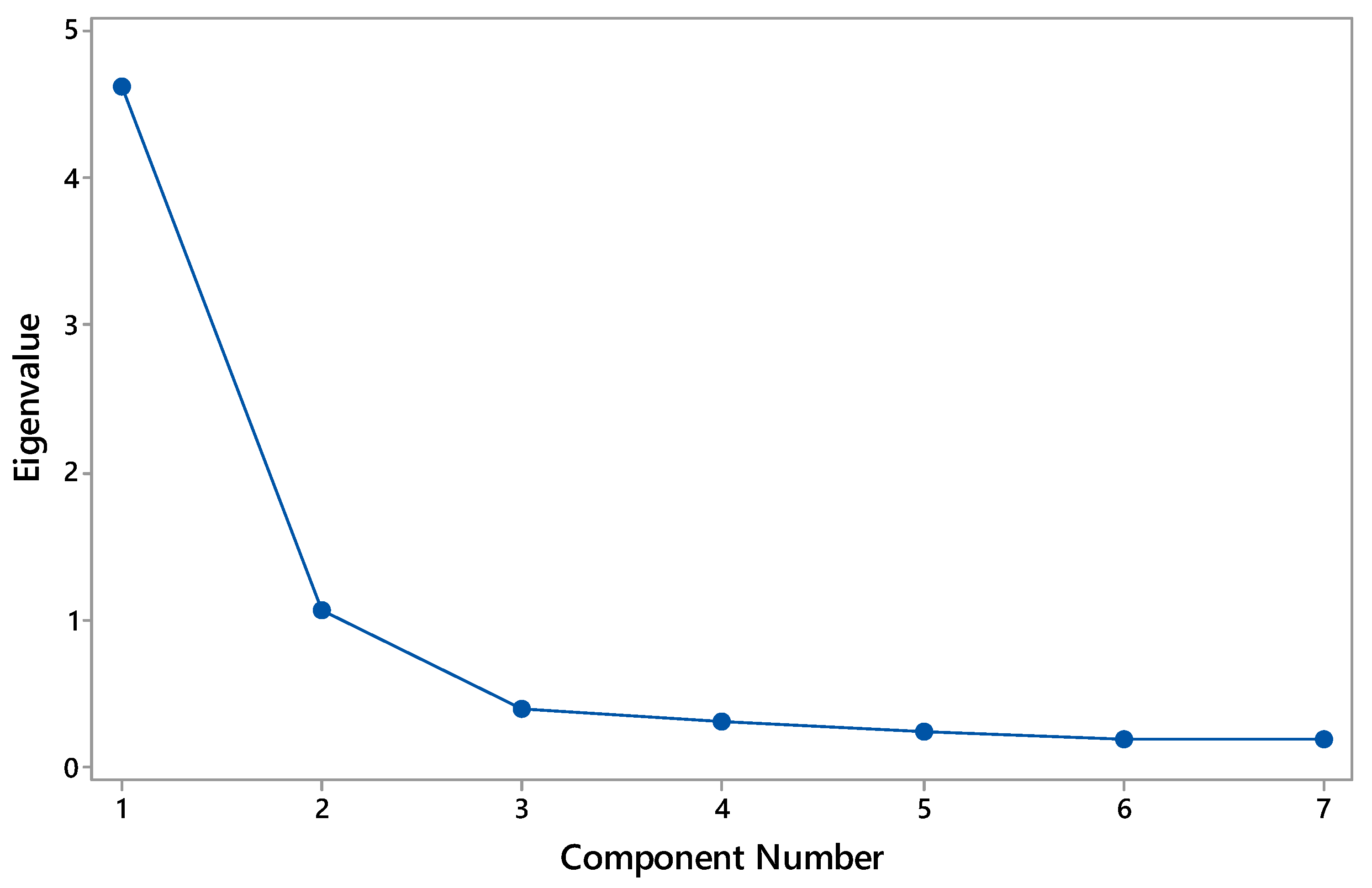
| Parameter | Inputs | ||||||
|---|---|---|---|---|---|---|---|
| PCA 1 | PCA 2 | PCA 3 | PCA 4 | PCA 5 | PCA 6 | PCA 7 | |
| Eigenvalue | 4.6162 | 1.0666 | 0.3896 | 0.3151 | 0.2323 | 0.1937 | 0.1865 |
| Proportion | 0.659 | 0.152 | 0.056 | 0.045 | 0.033 | 0.028 | 0.027 |
| Cumulative | 0.659 | 0.812 | 0.867 | 0.913 | 0.946 | 0.973 | 1 |
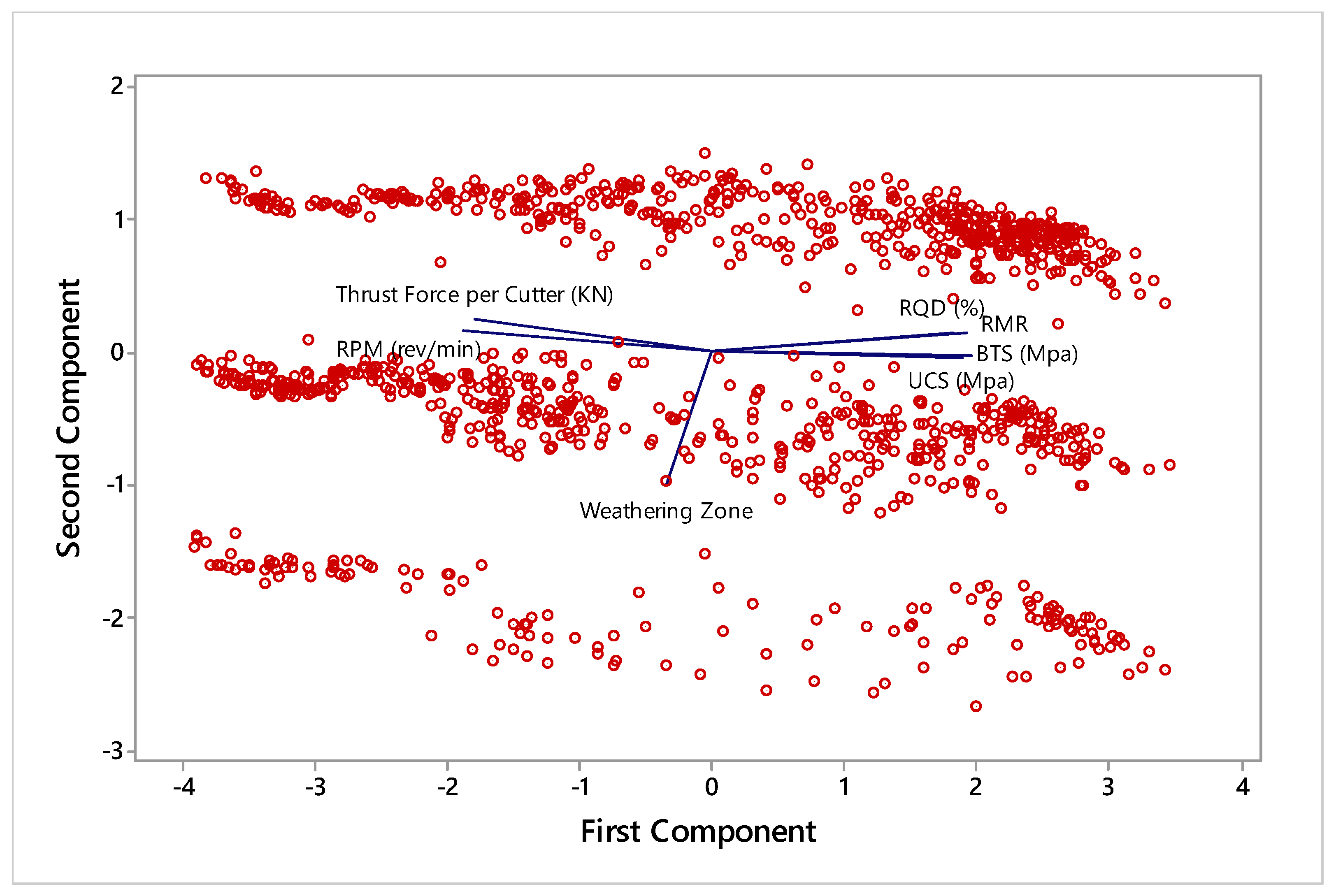
| Variable | Unit | PCA 1 | PCA 2 | PCA 3 | PCA 4 | PCA 5 | PCA 6 | PCA 7 |
|---|---|---|---|---|---|---|---|---|
| RQD | (%) | 0.397 | 0.138 | 0.369 | 0.737 | 0.048 | 0.331 | 0.181 |
| UCS | (MPa) | 0.424 | −0.031 | −0.151 | −0.159 | −0.433 | 0.433 | −0.629 |
| RMR | (-) | 0.417 | 0.128 | 0.317 | −0.019 | −0.338 | −0.766 | −0.092 |
| BTS | (MPa) | 0.412 | −0.035 | −0.517 | −0.129 | −0.293 | 0.056 | 0.675 |
| WZ | (-) | −0.074 | −0.941 | 0.07 | 0.23 | −0.21 | −0.083 | 0.009 |
| TFPC | (kN) | −0.388 | 0.235 | −0.499 | 0.573 | −0.383 | −0.202 | −0.174 |
| RPM | (rev/min) | −0.405 | 0.146 | 0.469 | −0.185 | −0.648 | 0.256 | 0.276 |
| Num | Topology | Num | Topology | Num | Topology | Num | Topology | Num | Topology |
|---|---|---|---|---|---|---|---|---|---|
| 1 | 1-1 | 5 | 2-1 | 9 | 3-1 | 13 | 4-1 | 17 | 5-1 |
| 2 | 1-2 | 6 | 2-2 | 10 | 3-1 | 14 | 4-2 | 18 | 5-2 |
| 3 | 1-3 | 7 | 2-3 | 11 | 3-3 | 15 | 4-3 | 19 | 5-3 |
| 4 | 1-4 | 8 | 2-4 | 12 | 3-4 | 16 | 4-4 | 20 | 5-4 |
| Number of Bees | Source Number of Bees | Max of Cycle Number | Onlooker Number |
|---|---|---|---|
| 10 | 5 | 50 | 5 |
| Neural Network’s Features | |||||
|---|---|---|---|---|---|
| Number of Inputs | Number of Outputs | Number of Hidden Layers | Number of Nodes in Hidden Layers | Transfer Function | Training Algorithm |
| 5 | 1 | 2 | 5-4 | tansig | Translim |
| Step | Statistical Index | PCA-ABC-ANN 2L (5-4) |
|---|---|---|
| Train | RMSE | 0.11 |
| AAE | 0.12 | |
| VAF% | 96% | |
| Test | RMSE | 0.12 |
| AAE | 0.13 | |
| VAF% | 96% |
| IW | b1 | ||||
|---|---|---|---|---|---|
| 1.0000 | 0.0048 | −1.0000 | −0.6979 | −0.3815 | |
| −0.7198 | 0.0175 | −0.0788 | −0.6253 | 0.9675 | |
| −1.0000 | 0.1828 | −0.8656 | −0.4221 | −0.6311 | |
| −1.0000 | 0.1674 | 1.0000 | 0.5205 | 0.7721 | |
| −0.4443 | 0.3115 | 1.0000 | −0.5144 | 0.5210 | |
| LW1 | b2 | ||||
| −0.8369 | 0.6940 | 1.0000 | −0.0327 | 0.1430 | 0.9120 |
| −0.4156 | 0.0648 | 1.0000 | 0.4767 | −0.3320 | −0.4661 |
| −0.0545 | 0.6210 | −1.0000 | −0.6569 | 0.3856 | 0.6196 |
| 1.0000 | −1.0000 | −0.0477 | 1.0000 | 0.7499 | 0.1558 |
| LW2 | b3 | ||||
| 0.3997 | 0.4148 | −0.5161 | −0.0175 | 0.1067 | |
| Models | R2% | Parameters | Equation Numbers |
|---|---|---|---|
| AR = 0.6405 − 0.002603 RQD − 0.001639 UCS − 0.006375 RMR − 0.00789 BTS − 0.00058 WZ + 0.002999 TFPC + 0.04854 RPM | 91.79 | 7 | (7) |
| AR = 0.6373 − 0.002600 RQD − 0.001639 UCS − 0.006364 RMR − 0.00788 BTS + 0.003002 TFPC + 0.04858 RPM | 91.68 | 6 | (8) |
| AR = 0.4662 − 0.002889 RQD (%) − 0.007356 RMR − 0.01365 BTS + 0.003159 TFPC + 0.05414 RPM | 91.39 | 5 | (9) |
| AR = 0.4266 − 0.009943 RMR − 0.01539 BTS + 0.003239 TFPC + 0.06152 RPM | 90.66 | 4 | (10) |
| AR = 1.7366 − 0.016681 RMR − 0.02506 BTS + 0.09089 RPM | 82.45 | 3 | (11) |
| AR = 0.5165 − 0.05625 BTS + 0.12752 RPM | 73.29 | 2 | (12) |
| AR = −0.7618 + 0.20618 RPM | 67.04 | 1 | (13) |
| Step | Statistical Index | PCA-ABC-ANN 2L (5-4) | PCA-ICA-ANN 2L (5-4) | MLR 7 |
|---|---|---|---|---|
| All | RMSE | 0.11 | 0.16 | 0.16 |
| AAE | 0.12 | 0.17 | 0.16 | |
| VAF% | 96% | 92% | 92% |
| Models’ Name | Employed Initialization Parameters in ICA | ||
|---|---|---|---|
| Number of Countries | Number of Imperialists | Number of Decades | |
| PCA-ICA-ANN 2L (5-4) | 500 | 50 | 250 |
Publisher’s Note: MDPI stays neutral with regard to jurisdictional claims in published maps and institutional affiliations. |
© 2022 by the authors. Licensee MDPI, Basel, Switzerland. This article is an open access article distributed under the terms and conditions of the Creative Commons Attribution (CC BY) license (https://creativecommons.org/licenses/by/4.0/).
Share and Cite
Wang, J.; Mohammed, A.S.; Macioszek, E.; Ali, M.; Ulrikh, D.V.; Fang, Q. A Novel Combination of PCA and Machine Learning Techniques to Select the Most Important Factors for Predicting Tunnel Construction Performance. Buildings 2022, 12, 919. https://doi.org/10.3390/buildings12070919
Wang J, Mohammed AS, Macioszek E, Ali M, Ulrikh DV, Fang Q. A Novel Combination of PCA and Machine Learning Techniques to Select the Most Important Factors for Predicting Tunnel Construction Performance. Buildings. 2022; 12(7):919. https://doi.org/10.3390/buildings12070919
Chicago/Turabian StyleWang, Jiangfeng, Ahmed Salih Mohammed, Elżbieta Macioszek, Mujahid Ali, Dmitrii Vladimirovich Ulrikh, and Qiancheng Fang. 2022. "A Novel Combination of PCA and Machine Learning Techniques to Select the Most Important Factors for Predicting Tunnel Construction Performance" Buildings 12, no. 7: 919. https://doi.org/10.3390/buildings12070919
APA StyleWang, J., Mohammed, A. S., Macioszek, E., Ali, M., Ulrikh, D. V., & Fang, Q. (2022). A Novel Combination of PCA and Machine Learning Techniques to Select the Most Important Factors for Predicting Tunnel Construction Performance. Buildings, 12(7), 919. https://doi.org/10.3390/buildings12070919