Relationship between Project Space Types, Optimize Energy Performance Credit, and Project Size in LEED-NC Version 4 (v4) Projects: A Case Study

Abstract

A previous study (Pushkar 2021) showed a significant non-parametric correlation between the Optimize Energy Performance credit from the energy and atmosphere category (EAc7) and project size in Leadership in Energy and Environmental Design for New Construction and Major Renovations version 4 (LEED-NC v4) office space projects. However, in such an empirical analysis, there are at least two problems: the choice between parametric and non-parametric statistics, and the choice between the Wilcoxon–Mann–Whitney (WMW) and analysis of covariance (ANCOVA) non-parametric tests. This study aims to evaluate EAc7 credit achievement for different types of spaces in LEED-NC v4 projects. We show that, in order to evaluate the differences between two LEED data groups, (1) a non-parametric procedure is preferable to a parametric one, and (2) if there is Spearman’s correlation between EAc7 credit achievement and project size for the same LEED-NC v4 project, then Quade’s ANCOVA is preferable to WMW. The results of these tests show that, in two out of three cases, office space projects had better EAc7 credit achievement than higher-education spaces at the gold certification level and public assembly spaces at the silver certification level.

1. Introduction

As Leadership in Energy and Environmental Design (LEED) certification has grown in popularity, numerous empirical analyses of LEED-certified projects have been published. This is because the LEED certification cannot be unified for different countries, certification levels, project types, or project sizes. Therefore, it is important to explore these factors. Such research can help LEED managers to determine the most appropriate certification strategy, taking into account their usually limited project-related budget and schedule [1]. However, these analyses require the use of the correct statistical tests, otherwise, the risk of reaching the wrong conclusion seems inevitable.

The LEED for New Construction and Major Renovations version 1 (LEED-NC v1) green rating system was launched in 1998 in the US; version 4 (v4) was introduced in 2013 after version 2.0 (v2 2000), version 2.2 (v2.2 2002), and version 3 (v3 2009) [2]. LEED-NC v4 contains four levels of certification: certified (40–49 points), silver (50–59 points), gold (60–79 points), and platinum (80–110 points) [3]. LEED-NC v4 contains seven main categories with maximum achievement points: integrative process credits (IP, 1 point), location and transportation (LT, 16 points), sustainable sites (SS, 10 points), water efficiency (WE, 11 points), energy and atmosphere (EA, 33 points), materials and resources (MR, 13 points), and indoor environmental quality (EQ, 16 points), along with two additional categories: regional priority (RP, 4 points) and innovation (IN, 6 points). In the last two LEED-NC versions (v3 and v4), the EA category contains one key credit—the Optimize Energy Performance credit (EAc), which was coded as EAc1 in v3 and EAc7 in v4, with a maximum of 19 and 18 points, respectively [3,4].

It was previously shown [5] that, in LEED-NC v3 2009 gold projects, the EAc1 credit was significantly higher in Finland and Sweden than in Turkey and Spain. It is possible that the reason for the different values of this credit is the significant differences in LEED-NC v3 2009 gold-type space projects in Finland and Sweden compared to Turkey and Spain [5].

Wu et al. [6] studied LEED for Neighborhood Development (LEED-ND) projects. They showed a significant non-parametric Spearman’s correlation between the achievement of 11 individual credits and total credits when transitioning between levels of certification. However, when they used the Kruskal–Wallis test to evaluate the statistical differences among the certified, silver, gold, and platinum groups, they showed that only 5 of 11 credits had $p$-values smaller than 0.05. In this context, we assumed that if there is a significant relationship between the achievement of individual LEED-ND credits and the overall LEED-ND score—i.e., the problem of the part-to-whole ratio—then ignoring this relationship could skew the results of the Kruskal–Wallis test. We also assumed that, so as to avoid the influence of correlation between individual credit achievements and total score in LEED-ND projects on the statistical differences among certified, silver, gold, and platinum groups, one-way non-parametric analysis of covariance (ANCOVA) can be used. Fisher [7] reported on applying ANCOVA to address the “problems concerned with the relation of a part to the whole”.

A significant relationship between EAc7 credit achievement and project size in LEED-NC v4 office-type projects at both the silver and gold certification levels was shown previously [8]. Therefore, when it is necessary to statistically determine, for example, the cross-certification performance between LEED-NC v4 certification levels, or between two types of spaces in LEED-NC v4 projects, the impact of project size on EAc7 credit achievement should be considered using ANCOVA. Therefore, to date, the use of ANCOVA to determine the differences between two or more groups of LEED projects when there is a correlation between the studied credit achievement and the project size from the same LEED project in each group has not yet been studied. The purpose of this study was to evaluate EAc7 credit achievement for different types of spaces in LEED-NC v4 projects.

2. Materials and Methods

2.1. Sample Size Assumption

To compare the differences between two independent groups—i.e., two types of spaces in LEED-NC v4 projects—we used the following parametric and non-parametric procedures: Student’s $t$-test versus exact Wilcoxon–Mann–Whitney (WMW) test [9], and Fisher’s versus Quaid’s ANCOVA [10,11]. Pearson’s versus Spearman’s correlation tests were used as assumptions to transit from Student’s/WMW tests to Fisher/Quaid ANCOVA tests when two independent groups were compared. Therefore, the minimum sample size (n) for the current study was determined based on the minimum sample size for conducting non-parametric tests [12]. According to Mundry and Fischer [13], for the exact WMW test, n ≥ 16, while for Spearman’s correlation n ≥ 20. Regarding non-parametric ANCOVA, Vickers [14] noted that “there is no simple relationship between relative power and sample size”. Therefore, based on the minimal sample for Spearman’s correlation, n = 20, we assumed that if n ≥ 21 in each group, then such a sample size can be acceptable for non-parametric ANCOVA.

2.2. Design of the Study

For a dose–response study, it is necessary to minimize the influence of uncontrolled factors on the object of study [15]. To accomplish this, we collected LEED-NC v4 projects in only one region—the US—sorted by type of space and level of certification. Large LEED-NC v4 projects in one group that did not appear in the other group were excluded from the analysis. Achievements of the LEED-NC v4 Optimize Energy Performance credit and project size were analyzed.

2.3. Data Collection

The US Green Building Council (USGBC) website [16] and the Green Building Information Gateway (GBIG) website [17] were used to collect US-LEED-NC v4 projects with different types of spaces. Table 1 shows that US-LEED-NC v4 includes 18 types of spaces and 4 levels of certification. In the present study, we focused on EAc7 credit achievement. Based on [8], LEED-NC v4 projects with a sample size of n = 21 or more were included in the statistical analysis, as shown in Table 1.

Table 1. US-LEED-NC v4 projects, in alphabetical order (accessed on 14 January 2022).

Serial Number	LEED-NC v4 Type of Space	Number of US-LEED-NC v4 Projects
		Certified	Silver	Gold	Platinum
1	Data center	1	0	0	0
2	Educational facility	0	5	1	0
3	Health care	4	4	6	0
4	Higher education	4	39	26	3
5	Industrial manufacturing	7	5	1	0
6	K-12	0	4	0	0
7	Laboratory	2	3	3	0
8	Lodging	5	3	0	0
9	Multi-family residential	12	10	7	0
10	Office	32	35	44	10
11	Other	6	9	7	1
12	Public assembly	21	25	11	0
13	Public order and safety	5	16	6	0
14	Religious worship	1	0	0	0
15	Retail	12	0	2	0
16	Service	2	4	1	0
17	Undefined	4	2	1	1
18	Warehouse and distribution	3	0	0	0

Note: bold font indicates acceptable numbers of projects (n ≥ 21).

Three LEED-NC v4 case projects were collected—Case 1: office space group 1.1 of n_1.1 = 32 versus public assembly space group 1.2 of n_1.2 = 21 at the certified level; Case 2: office space group 2.1 of n_2.1 = 44 versus higher-education space group 2.2 of n_2.2 = 26 at the gold level; and Case 3: office space group 3.1 of n_3.1 = 35 and public assembly space group 3.2 of n_3.2 = 25 at the silver level.

2.4. Corrected Sample Size

To avoid the influence of the extremely large LEED project size on EA credit achievement, in Case 1, from 32 projects of LEED-NC v4 certified office space projects, 1 project was excluded from the analysis (≥40,521 m²); in Case 2, from 44 projects of gold office space projects, 4 projects were excluded from the analysis (≥40,818 m²); and in Case 3, from 35 silver office space projects, 1 project was excluded from the analysis (≥65,497 m²). Thus, for Cases 1, 2, and 3, the maximum project sizes were 23,226, 23,783, and 23,094 m², respectively. A summary of the US-LEED-NC v4 projects is given in Table 2.

Table 2. Corrected sample sizes of US-LEED v4 projects.

Certification Level	Certified (Case 1)		Gold (Case 2)		Silver (Case 3)
LEED-NC v4 project	Office (group 1.1)	Public assembly (group 1.2)	Office (group 2.1)	Higher education (group 2.2)	Office (group 3.1)	Public assembly (group 3.2)
Sample size	31	21	40	26	34	25
Total sample size	52		66		59

In the present study, the following parametric and non-parametric statistical procedures were used: descriptive statistics, inferential statistics and assumptions, effect size, and $p$-value interpretations. The $p$-values are interpreted in Section 2.7 of this article.

2.5. Statistical Methods

2.5.1. Descriptive Statistics

LEED-NC v4 EAc7 credit achievement was noted as response variable Y, while project size was noted as covariate X. Variable Y, which is related to ordinal scale, and covariate X, which is related to interval scale, refer to the same LEED-NC v4 project. We used the means of response variable Y ± standard deviation (SD) and medians of response variable Y ± interquartile range (IQR, 25th–75th percentile) to describe parametric and non-parametric statistics, respectively.

2.5.2. Inferential Statistics

An unpaired two-tailed parametric Student’s $t$-test ($t$-test) and exact WMW test were performed to evaluate the differences between two unpaired groups. According to Bergmann et al. [9], if data contain ordinal or discrete interval variables with relatively few values, an exact WMW procedure—not an approximate one—should be used.

Parametric Pearson’s correlation and non-parametric Spearman’s correlation were used to evaluate the association between EAc7 credit achievement and project size for the same LEED-NC v4 projects.

Parametric Fisher’s ANCOVA [10] and non-parametric Quade’s ANCOVA [11] were used to evaluate the differences between two groups with respect to response variable Y when covariate X was taken into account [18].

2.5.3. Checking Assumptions When Using Parametric Tests

A prerequisite for using parametric statistics is that certain assumptions must be met. In general, if these assumptions do not hold, non-parametric statistics should be used [19].

Statistical Tests for Unpaired Groups and Assumptions

To perform a $t$-test, the following assumptions are made: assumption of normality of variables (Shapiro–Wilk test), equal variability assumption (Fisher–Snedecor F-test), and Satterthwaite’s approximate $t$-test if variances are not assumed to be equal.

Correlation Procedures and Gauss–Markov Assumptions

According to Boldina and Beninger [20], in order to determine Pearson’s correlation, five Gauss–Markov assumptions should be met: (1) linearity in form, as determined by visual inspection; (2) correlation between residuals and independent variables, evaluated by ordinary least squares; (3) autocorrelation, evaluated by the Durbin–Watson test; (4) homoscedasticity, evaluated by the Breusch–Pagan test; and (5) normality in residuals, evaluated by the Shapiro–Wilk test.

Assumptions for Using Fisher’s ANOVA

Five Gauss–Markov assumptions were used [20]. In addition, the non-parametric triples test was used to evaluate the asymmetry assumption [21], and the Fisher–Snedecor F-test was used to evaluate the homogeneity assumption of variance [22].

2.6. Effect Size Interpretation

Parametric Cohen’s $d$ with bias correction was used to measure the effect size of the difference between two means [23]. Cohen’s $d$ can take on any number between 0 and infinity. The effect size is considered to be negligible if $d$ < 0.20, small if 0.20 ≤ $d$< 0.50, medium if 0.50 ≤ $d$ < 0.80, and large if $d$ ≥ 0.80 [24].

Non-parametric Cliff’s $\delta$ was applied to measure the effect size of the difference between two distributions [25]. Cliff’s $\delta$’s effect size ranges between −1 and +1. Positive (+) values indicate that group 1 is larger than group 2, 0 indicates equality or overlap, and negative (−) values indicate that group 2 is larger than group 1 [25]. The effect size is negligible if |$\delta$| < 0.147, small if 0.147 ≤ |$\delta$| < 0.33, medium if 0.33 ≤ |$\delta$| < 0.474, and large if |$\delta$| ≥ 0.474 [26].

2.7. p-Value Interpretation

As recommended by Hurlbert and Lombardi [27], the paleo-Fisherian and Neyman–Pearsonian paradigms (null hypothesis significance tests (NHSTs)) were replaced by neo-Fisherian significance assessments (NFSAs). According to Hurlbert and Lombardi [27], the NFSA (1) does not fix $\alpha$, (2) does not describe $p$-values as significant or non-significant, (3) does not accept the null hypothesis based on high $p$-values, but only suspends judgment, (4) interprets significance tests according to 3-valued logic, and (5) presents effect size information if necessary.

Hurlbert and Lombardi [27] cite a recommendation by Gotelli and Ellison [28], noting that “in many cases, it may be more important to report the exact $p$-value and let the readers decide for themselves how important the results are”. According to Beninger et al. [29], the logic of Occam’s razor should not be used for universal interpretation of $p$-values.

Hurlbert and Lombardi [27] clearly showed that fixing $\alpha$ (the level of significance; e.g., $\alpha$ = 0.05) and dichotomizing the scale of $p$-values (i.e., $p$ < $\alpha$ or $p$ > $\alpha$) are superfluous. They cited Fischer’s philosophical proposal that “no scientific worker has a fixed level of significance at which from year to year, and in all circumstances, he rejects (null) hypotheses; he rather gives his mind to each particular case in light of his evidence and ideas” [30]. In addition, Altman [19] noted that “It is ridiculous to interpret the results of a study differently according to whether the $p$-value obtained was, say, 0.055 or 0.045. These $p$-values should lead to very similar conclusions, not diametrically opposed ones”.

According to Hurlbert and Lombardi [27], for NFSAs, precise $p$-values are evaluated and shown according to a three-valued logic: seems to be positive (i.e., there seems to be a difference between group 1 and group 2), seems to be negative (i.e., there does not seem to be a difference between the groups), or judgment is suspended regarding the difference between groups 1 and 2.

3. Results and Discussion

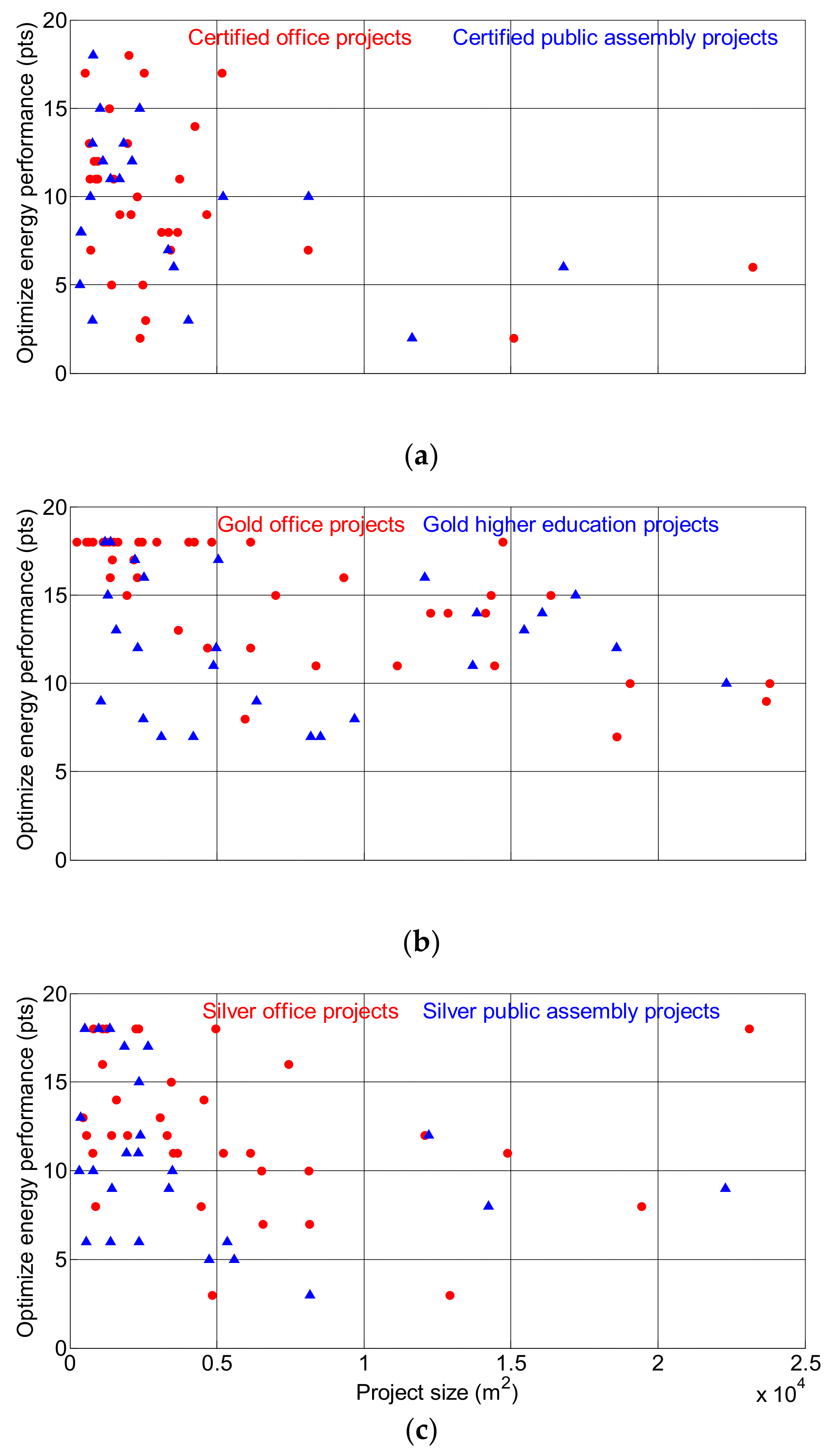
3.1. Visual Analysis

Visual analysis of all three cases in Figure 1 shows that a larger LEED-NC v4 project size is associated with a monotonic decrease in the EAc7 credit.

Figure 1. Relationship between LEED-NC v4 project size and Optimize Energy Performance credit in three cases of project spaces: (a) office (red circle) and public assembly (blue triangle) projects at the certified level (top panel), (b) office (red circle) and higher-education (blue triangle) projects at the gold level (middle panel), and (c) office (red circle) and public assembly (blue triangle) projects at the silver level (bottom panel).

Thus, project size might be considered as an influential factor when comparing different space types with regard to this credit. Section 3.2 presents a detailed statistical analysis of this issue for the three studied cases.

This correlation between EAc7 credit achievement and project size in LEED-NC v4 projects was first revealed in [8]. In that study, it was noted that the types of envelope construction and heating, ventilation, and air-conditioning (HVAC) equipment installed are different for small and large office spaces. In particular, it is recommended that small offices be built with mass walls and an average window-to-wall ratio of 19%, while large offices should be built with a steel frame or mass walls and an average window-to-wall ratio of 54% [31]. In small offices, flexible refrigerant-based packaged air-conditioning units for air cooling and heating are usually installed, while in large offices, centralized water-based air-cooling chillers and air-heating boilers are implemented [32]. Thus, as was concluded in [8], smaller offices are more likely to have more insulation and to be more effectively equipped with HVAC systems to save cooling and heating energy and obtain more points for the EAc7.

In the present study, this correlation between EAc7 credit achievement and size in LEED-NC v4 projects was confirmed for office spaces and expanded for higher-education and public assembly spaces. This highlights the importance of taking this correlation into account when distinguishing between LEED-NC v4 projects based on the type of space.

3.2. Statistical Analysis

3.2.1. Case 1

In Case 1, we analyzed the differences in EAc7 credit achievement between office space group 1.1 and public assembly space group 1.2 at the LEED-NC certified level. The comparisons of the EAc7 performance of groups 1.1 and 1.2 without and with considering project size are presented in Table 3 and Table 4, respectively.

Table 3. Case 1: comparison of EAc7 (Optimize Energy Performance) credit achievement of groups 1.1 and 1.2 without considering project size in LEED-NC v4 certified projects.

Type of Space for LEED Project	Descriptive Statistics		Inferential Statistics
	Mean ± STD	Median, 25th–75th Percentiles	Assumption of Normality p-Value	Parametric t-Test, p-Value (Cohen’ d)	Non-Parametric WMW Test, p-Value (Cliff’ δ)
Office (group 1.1)	9.9 ± 4.4	10.0, 7.0–12.8	0.5449 a	0.6807 a (0.11)	0.7561 a (0.05)
Public assembly (group 1.2)	9.4 ± 4.3	10.0, 6.0–12.3	0.8551 a

$p$-values were evaluated according to three-valued logic; ^a Roman font indicates that the value seems to be negative.

Table 4. Case 1: comparison of EAc7 (Optimize Energy Performance) credit achievement of groups 1.1 and 1.2 when considering project size in LEED-NC v4 certified projects.

Correlation between	Type of Space for LEED Project	Parametric Statistics			Non-Parametric Statistics
		Pearson’s Product–Moment Correlation, $\mathit{p}$-Value	Fisher’s ANCOVA, $\mathit{p}$-Value		Spearman’s Rank-Order Correlation, p-Value	Quade’s ANCOVA, p-Value
EAc7 and project size	Office (group 1.1)	0.0518b	Difference between groups 1.1 and 1.2	0.7958 a	0.0465b	Difference between group 1.1 and group 1.2	0.5520 a
	Public assembly (group 1.2)	0.0784 a			0.4244 a

$p$-values were evaluated according to three-valued logic; ^a Roman font indicates that the value seems to be negative; ^b italic font indicates that judgment is suspended.

Table 3 shows that the assumption of normality was met in both groups ($p$ = 0.5449 and $p$ = 0.8551, respectively). In this context, $t$-tests and exact WMW tests showed similar results: the difference between groups 1.1 and 1.2 seemed to be negative ($p$ = 0.6807 and $p$ = 0.7561, respectively), and the effect size in both tests was negligible (Cohen’s $d$ = 0.11 and Cliff’s $\delta$ = 0.05).

It was shown that four Gauss–Markov assumptions and two Fisher’s ANCOVA assumptions (0.0795 ≤ $p$ ≤ 1.0000) were met in groups 1.1 and 1.2 (Appendix A, Table A1). As can be seen in Table 4, despite the fact that the above assumptions were met, in group 1.1, Pearson’s and Spearman’s correlations showed similar results—suspended judgment regarding the correlation between EAc7 credit achievement and project size ($p$ = 0.0518 and $p$ = 0.0465, respectively)—while in group 1.2, Pearson’s and Spearman’s correlations showed similar results, appearing to be negative ($p$ = 0.0784 and $p$ = 0.4244, respectively). As we can see in Table 4, Fisher’s and Quade’s ANCOVA tests showed similar results: the difference between groups 1.1 and 1.2 seemed to be negative ($p$ = 0.7958 and $p$ = 0.5520, respectively).

3.2.2. Case 2

In Case 2, we analyzed the differences in EAc7 credit achievement between office space group 2.1 and higher-education space group 2.2 at the LEED-NC gold level. Comparisons of the EAc7 performance of the two groups without and with considering project size are presented in Table 5 and Table 6, respectively.

Table 5. Case 2: comparisons of EAc7 (Optimize Energy Performance) credit achievement for groups 2.1 and 2.2 without considering project size in LEED-NC v4 gold projects.

Type of Space for LEED Project	Descriptive Statistics		Inferential Statistics
	Mean ± STD	Median, 25th–75th Percentiles	Assumption of Normality, p-Value	Parametric t-Test, p-Value (Cohen’s d)	Non-Parametric WMW Test, p-Value (Cliff’s δ)
Office (group 2.1)	15.1 ± 3.3	16.0, 12.5–18.0	0.00003a	0.0013a (0.83)	0.0011a (0.47)
Higher education (group 2.2)	12.2 ± 3.7	12.0, 9.0–15.0	0.0929 b

$p$-values were evaluated according to three-valued logic; ^a bold font indicates that the value seems to be positive; ^b Roman font indicates that the value seems to be negative.

Table 6. Case 2: comparisons of EAc7 (Optimize Energy Performance) credit achievement for groups 2.1 and 2.2 considering project size in LEED-NC v4 gold projects.

Correlation between	Type of Space for LEED Project	Parametric Statistics			Non-Parametric Statistics
		Pearson’s Product–Moment Correlation,$\mathit{p}$-Value	Fisher’s ANCOVA, p-Value		Spearman’s Rank-Order Correlation p-Value	Quade’s ANCOVA, p-Value
EAc7 and project size	Office (group 2.1)	0.000001a	Difference between group 2.1 and group 2.2	0.0122a	0.00001a	Difference between group 2.1 and group 2.2	0.0005a
	Higher education (group 2.2)	0.7249 b			0.4236 b

$p$-values were evaluated according to three-valued logic; ^a bold font indicates that the value seems to be positive; ^b Roman font indicates that the value seems to be negative.

Table 5 shows that the assumption of normality was not met for group 2.1 ($p$ = 0.00003) but was met for group 2.2 ($p$ = 0.0929). Although the $t$-test was not recommended in this context, $t$-tests and exact WMW tests showed similar results: the difference between groups 2.1 and 2.2 was positive ($p$ = 0.0013 and $p$ = 0.0011, respectively). In this case, the effect size was large in both tests (Cohen’s $d$ = 0.83 and Cliff’s $\delta$ = 0.47, respectively).

It was shown that in group 2.1, three of the four Gauss–Markov assumptions—autocorrelation in residuals ($p$ = 0.0412), homoscedasticity ($p$ = 0.00004), and normality in residuals ($p$ = 0.0055)—and one Fisher’s ANCOVA assumption—symmetry distribution ($p$ = 0.0003)—were not met, while in group 2.2, four Gauss–Markov assumptions and two ANCOVA assumptions were met (0.0874 ≤ $p$ ≤ 1.0000) (Appendix A, Table A2).

As can be seen in Table 6, although Pearson’s correlation and Fisher’s ANCOVA tests were not recommended in this context, Pearson’s and Spearman’s tests showed similar results: in group 2.1, the correlation between EAc7 credit achievement and project size seemed to be positive ($p$ = 0.000001 and $p$ = 0.00001, respectively), while in group 2.2 it seemed to be negative ($p$ = 0.7249 and $p$ = 0.4236, respectively), and Fisher’s and Quade’s ANCOVA tests seemed to show positive results: $p$ = 0.0122 and $p$ = 0.0005, respectively.

3.2.3. Case 3

In Case 3, we analyzed the differences in EAc7 achievement between office space group 3.1 and public assembly space group 3.2 at the LEED-NC silver level. The comparisons of the EAc7 performance of the two groups without and with considering project size are presented in Table 7 and Table 8, respectively.

Table 7. Case 3: comparison of EAc7 (Optimize Energy Performance) credit achievement of groups 3.1 and 3.2 without considering project size in LEED-NC v4 silver projects.

Type of Space for LEED Project	Descriptive Statistics		Inferential Statistics
	Mean ± STD	Median, 25th–75th Percentiles	Assumption of Normality, p-Value	Parametric t-Test, p-Value (Cohen’s d)	Non-Parametric WMW Test, p-Value (Cliff’s δ)
Office (group 3.1)	12.3 ± 4.2	12.0, 10.0–16.0	0.0384a	0.1410 b (0.38)	0.0863 b (0.26)
Public assembly (group 3.2)	10.6 ± 4.5	10.0, 6.0–13.5	0.0980 b

$p$-values were evaluated according to three-valued logic; ^a bold font indicates that the value seems to be positive; ^b Roman font indicates that the value seems to be negative.

Table 8. Case 3: comparison of EAc7 (Optimize Energy Performance) credit achievement of groups 3.1 and 3.2 considering project size in LEED-NC v4 silver projects.

Correlation between	Type of Space for LEED Project	Parametric Statistics			Non-Parametric Statistics
		Pearson’s Product–Moment Correlation,$\mathit{p}$-Value	Fisher’s ANCOVA, p-Value		Spearman’s Rank-Order Correlation p-Value	Quade’s ANCOVA, p-Value
EAc7 and project size	Office (group 3.1)	0.1974 b	Difference between group 3.1 and group 3.2	0.7306	0.0254a	Difference between group 3.1 and group 3.2	0.0162a
	Public assembly (group 3.2)	0.1696 b			0.0293a

$p$-values were evaluated according to three-valued logic; ^a bold font indicates that the value seems to be positive; ^b Roman font indicates that the value seems to be negative.

As can be seen in Table 7, in one of the groups, the assumption of normality was not met ($p$ = 0.0384). As a result, if the $t$-test was applied, the statistical difference between the two groups was $p$ = 0.141, with a small effect size (Cohen’s $d$ = 0.38), while if the exact WMW test was applied, the difference between the two groups was $p$ = 0.0863, with a small effect size (Cliff’s $\delta$ = 0.26); that is, in both tests, the difference between the two groups seemed to be negative.

It was shown that in group 3.1, the assumption of homoscedasticity was not met ($p$ = 0.0184), while in group 3.2, four Gauss–Markov and two Fisher ANCOVA assumptions were met (0.0685 ≤ $p$ ≤ 1.000) (Appendix A, Table A3).

Table 8 shows the results of parametric and non-parametric tests—Pearson’s correlation and Fisher’s ANCOVA results versus Spearman’s correlation and Quade’s ANCOVA results. The Pearson’s test results show that the correlation between EAc7 credit achievement and project size in both groups 3.1 and 3.2 seems to be negative ($p$ = 0.1974 and $p$ = 0.1696, respectively), and the Fisher’s ANCOVA results show that the difference between the two groups seems to be negative ($p$ = 0.7306). In contrast, the Spearman’s test results show that the correlation between EAc7 credit achievement and project size in both groups 3.1 and 3.2 seems to be positive ($p$ = 0.0254 and $p$ = 0.0293, respectively), and the Quade’s ANCOVA results show that the difference between the two groups seems to be positive ($p$ = 0.0162).

A critical analysis of the literature review (e.g., [33,34,35,36]) shows that, in general, LEED data should be treated using non-parametric statistics.

In this study, we compared the results of parametric and non-parametric statistics. As a result, Cases 2 and 3 showed that ignoring assumptions when using parametric statistics can result in erroneous statistical conclusions.

We showed that using the non-parametric ANCOVA test instead of the non-parametric WMW test may be more efficient for detecting differences between two independent groups with LEED-NC v4 data if there is a significant Spearman’s correlation between the EAc7 credit achievement and LEED-NC v4 project size in each group. Vickers [14] showed similar results for the treatment of abnormally distributed data.

In addition, three cases suggest that the use of ANCOVA could lead to new knowledge in green building rating systems:

• In a study by Pushkar and Verbitsky [37], LEED projects from eight US states were relocated from environmental categories to the building layer (BL) and service layer (SL). Spearman’s test results showed a significant and negative correlation between the BL and SL. Three design strategies were identified: BL-emphasized, SL-emphasized, and random [37]. However, this study did not assess the differences between US states. In this context, non-parametric Quade’s ANCOVA can be useful for the statistical measurement of differences between US states.
• Suzer [38] focused on 20 buildings dually certified by LEED-NC v4 and the Building Research Establishment Environmental Assessment Method (BREEAM) version 2014. Pearson’s test results showed a significant and large positive correlation between the total scores of LEED-NC v4 and BREEAM [38]. It should be noted that in a number of European countries, the LEED and BREEAM green rating systems are used in parallel for building certification. In this context, the differences between countries can be evaluated using non-parametric Quaid’s ANCOVA.
• ElBatran and Ismaeel [39], among others, studied the relationship between spatial daylight autonomy (sDA) and annual sunlight exposure (ASE) in office buildings with a double-skin façade. Using a parametric Pearson’s test, they showed that the relationship between sDA and ASE had a significant positive correlation ($p$ < 0.001). However, in this context, the differences between double-skin façade alternatives can be evaluated using Fisher’s ANCOVA.

4. Conclusions

• To evaluate LEED data, the use of non-parametric significance tests is preferred over parametric significance tests.
• To compare LEED data from two or more groups, it is necessary to test for logically possible correlations between variables in each group, and if a non-parametric correlation exists, then Quade’s ANCOVA is preferable to the exact WMW test.
• In two out of three cases, the EAc7 (Optimize Energy Performance) credit achievement in LEED-NC v4 projects was better in office-type projects than in higher-education-type projects at the gold level of certification, and in office-type projects than in public-type projects at the silver level.

References

- Cheng, J.C.P.; Ma, L.J. A study of the relationship between credits in the LEEDEB&OM green building rating system. IACSIT Int. J. Eng. Technol. 2013, 5, 438–442. [Google Scholar] [CrossRef]
- Ade, R.; Rehm, M. The unwritten history of green building rating tools: A personal view from some of the ‘founding fathers’. Build. Res. Inf. 2020, 48, 1–17. [Google Scholar] [CrossRef]
- LEED. LEED v4 for New Construction and Major Renovations. 2019. Available online: https://www.usgbc.org/sites/default/files/LEED%20v4%20BDC_07.25.19_current.pdf (accessed on 20 November 2020).
- LEED. LEED 2009 for New Construction and Major Renovations. 2014. Available online: https://energy.nv.gov/uploadedFiles/energynvgov/content/2009_NewConstruction.pdf (accessed on 18 November 2020).
- Pushkar, S. A Comparative Analysis of Gold Leadership in Energy and Environmental Design for New Construction 2009 Certified Projects in Finland, Sweden, Turkey, and Spain. Appl. Sci. 2018, 8, 1496. [Google Scholar] [CrossRef] [Green Version]
- Wu, P.; Song, Y.; Hu, X.; Wang, X. A Preliminary Investigation of the Transition from Green Building to Green Community: Insights from LEED ND. Sustainability 2018, 10, 1802. [Google Scholar] [CrossRef] [Green Version]
- Fisher, A. The Analysis of Covariance Method for the Relation between a Part and the Whole. Biometrics 1947, 3, 65–68. [Google Scholar] [CrossRef]
- Pushkar, S. Relationship between Energy and Atmosphere (EA) Credits and Project Size in the LEED-NC Version 3 (v3) and 4 (v4) Projects. Buildings 2021, 11, 114. [Google Scholar] [CrossRef]
- Bergmann, R.; Ludbrook, J.; Spooren, W.P.J.M. Different outcomes of the Wilcoxon-Mann-Whitney test from different statistics packages. Am. Stat. 2000, 54, 72–77. [Google Scholar] [CrossRef]
- Fisher, R.A. Statistical Methods for Research Workers; Oliver & Boyd: Edinburgh, UK, 1932. [Google Scholar]
- Quade, D. Rank analysis of covariance. J. Am. Stat. Assoc. 1967, 63, 1187–1200. [Google Scholar] [CrossRef]
- Chin, R.; Lee, B.Y. Principles and Practice of Clinical Trial Medicine; Elsevier: Amsterdam, The Netherlands, 2008. [Google Scholar]
- Mundry, R.; Fischer, J. Use of statistical programs for nonparametric tests of small samples often leads to incorrect p values: Examples from animal behaviour. Anim. Behav. 1998, 56, 256–259. [Google Scholar] [CrossRef] [Green Version]
- Vickers, A.J. Parametric versus non-parametric statistics in the analysis of randomized trials with non-normally distributed data. BMC Med. Res. Methodol. 2005, 5, 35. [Google Scholar] [CrossRef] [Green Version]
- Hurlbert, S.H. Pseudoreplication and the Design of Ecological Field Experiments. Ecol. Monogr. 1984, 54, 187–211. [Google Scholar] [CrossRef] [Green Version]
- USGBC Projects Site. Available online: https://www.usgbc.org/projects (accessed on 14 January 2022).
- GBIG Green Building Data. Available online: http://www.gbig.org (accessed on 14 January 2022).
- Rae, G. Quade’s nonparametric analysis of covariance by matching. Behav. Res. Methods Instrum. Comput. 1985, 17, 421–422. [Google Scholar] [CrossRef]
- Altman, D.G. Practical Statistics for Medical Research; Chapman and Hall (Monograph): London, UK, 1991. [Google Scholar]
- Boldina, I.; Beninger, P.G. Strengthening statistical usage in marine ecology: Linear regression. J. Exp. Mar. Biol. Ecol. 2016, 474, 81–91. [Google Scholar] [CrossRef]
- Randles, R.H.; Fligner, M.A.; Policello, G.E.; Wolfe, D.A. An asymptotically distribution-free test for symmetry versus asymmetry. J. Am. Stat. Assoc. 1980, 75, 168–172. [Google Scholar] [CrossRef]
- Snedecor, G.W.; Cochran, W.G. Statistical Methods; Iowa State University Press: Ames, IA, USA, 1967. [Google Scholar]
- Hedges, L.V. Distribution Theory for Glass’s Estimator of Effect Size and Related Estimators. J. Educ. Stat. 1981, 6, 107–128. [Google Scholar] [CrossRef]
- Cohen, J. A power primer. Psychol. Bull. 1992, 112, 155–159. [Google Scholar] [CrossRef]
- Cliff, N. Dominance statistics: Ordinal analyses to answer ordinal questions. Psychol. Bull. 1993, 114, 494–509. [Google Scholar] [CrossRef]
- Romano, J.; Corragio, J.; Skowronek, J. Appropriate statistics for ordinal level data: Should we really be using t-test and Cohen’s d for evaluating group differences on the NSSE and other surveys? In Proceedings of the Annual Meeting of the Florida Association of Institutional Research, Cocoa Beach, FL, USA, 1–3 February 2006; Florida Association for Institutional Research: Cocoa Beach, FL, USA, 2006; pp. 1–33. [Google Scholar]
- Hurlbert, S.H.; Lombardi, C.M. Final collapse of the Neyman-Pearson decision theoretic framework and rise of the neoFisherian. Ann. Zool. Fenn. 2009, 46, 311–349. Available online: https://www.jstor.org/stable/23736900 (accessed on 20 April 2022). [CrossRef]
- Gotelli, N.J.; Ellison, A.M. A Primer of Ecological Statistics; Sinauer Associates: Sunderland, MA, USA, 2004. [Google Scholar]
- Beninger, P.G.; Boldina, I.; Katsanevakis, S. Strengthening statistical usage in marine ecology. J. Exp. Mar. Biol. Ecol. 2012, 426–427, 97–108. [Google Scholar] [CrossRef]
- Fisher, R.A. Statistical Methods and Scientific Inference; Hafner Publishing Co.: Oxford, UK, 1956. [Google Scholar]
- Winiarski, D.W.; Halverson, M.A.; Jiang, W. Analysis of Building Envelope Construction in 2003 CBECS. Prepared for the U.S. Department of Energy under Contract DE-AC05-76RL01830. Pacific Northwest National Laboratory. 2007. Available online: https://www.pnnl.gov/main/publications/external/technical_reports/PNNL-20380.pdf (accessed on 20 April 2022).
- Winiarski, D.W.; Jiang, W.; Halverson, M.A. Review of Pre- and Post-1980 Buildings in CBECS—HVAC Equipment. Prepared for the U.S. Department of Energy under Contract DE-AC05-76RL01830. Pacific Northwest National Laboratory. 2006. Available online: https://www.pnnl.gov/main/publications/external/technical_reports/PNNL-20346.pdf (accessed on 20 April 2022).
- Pham, D.H.; Kim, B.; Lee, J.; Ahn, Y. An Investigation of the Selection of LEED Version 4 Credits for Sustainable Building Projects. Appl. Sci. 2020, 10, 7081. [Google Scholar] [CrossRef]
- Chi, B.; Lu, W.; Ye, M.; Bao, Z.; Zhang, X. Construction waste minimization in green building: A comparative analysis of LEED-NC 2009 certified projects in the US and China. J. Clean. Prod. 2020, 256, 120749. [Google Scholar] [CrossRef]
- Wu, P.; Mao, C.; Wang, J.; Song, Y.; Wang, X. A decade review of the credits obtained by LEED v2.2 certified green building projects. Build. Environ. 2016, 102, 167–178. [Google Scholar] [CrossRef]
- Wu, P.; Song, Y.; Shou, W.; Chi, H.; Chong, H.Y.; Sutrisna, M. A comprehensive analysis of the credits obtained by LEED 2009 certified green buildings. Renew. Sustain. Energy Rev. 2017, 68, 370–379. [Google Scholar] [CrossRef]
- Pushkar, S.; Verbitsky, O. Strategies for LEED certified projects: The building layer versus the service layer. Can. J. Civ. Eng. 2018, 45, 1065–1072. [Google Scholar] [CrossRef]
- Suzer, O. Analyzing the compliance and correlation of LEED and BREEAM by conducting a criteria-based comparative analysis and evaluating dual certified projects. Build. Environ. 2019, 147, 158–170. [Google Scholar] [CrossRef]
- ElBatran, R.M.; Ismaeel, W.S.E. Applying a parametric design approach for optimizing daylighting and visual comfort in office buildings. Ain Shams Eng. J. 2021, 12, 3275–3284. [Google Scholar] [CrossRef]
Publisher’s Note: MDPI stays neutral with regard to jurisdictional claims in published maps and institutional affiliations. |
© 2022 by the author. Licensee MDPI, Basel, Switzerland. This article is an open access article distributed under the terms and conditions of the Creative Commons Attribution (CC BY) license (https://creativecommons.org/licenses/by/4.0/).