1. Introduction
The increasing global energy demand, the anticipated reduction in available fossil fuels, and the increasing evidence of global warming during the last decades have generated a high interest in renewable energy sources and integration of renewable energy sources into the power grid is increasing rapidly worldwide. However, renewable energy sources, such as wind and solar power, have an inherent variability that can seriously affect the stability of the energy system if they account for a high percentage of the total generation. The flexibility to manage any mismatch between consumption and generation can come from either the supply side through the use of conventional power plants or storage [
1,
2,
3,
4] or from the demand side [
5,
6,
7,
8]. The concept of an energy flexible building (EFB) was initiated and studied by IEA EBC Annex 67 [
9]. The current definition of building energy flexibility based on the Annex 67 is “the ability to manage building demand and generation according to local climate conditions, user needs, and energy network requirements” [
9]. The flexibility of building energy demand profiles is commonly suggested as part of the solution to alleviate some of the upcoming challenges in the future demand response energy systems [
9]. Knowledge of energy flexibility that buildings can provide is important for the design of future smart energy systems, smart grids, and buildings. The knowledge is, however, not only important for utilities but also for companies when developing business cases for products and services supporting the roll out of smart energy networks. Furthermore, it is important for policy makers and government entities involved in the shaping of future energy systems. Radiant floor systems offer significant potential for studying and developing energy flexibility strategies for buildings and their interaction with smart grids. Efficient design and operation of such systems require several critical decisions on design and control variables to maintain comfortable thermal conditions in the space and floor surface temperatures within the recommended range. There have been recent studies on activating and utilizing the energy flexibility of zones with radiant heating systems by means of predictive control strategies [
10,
11,
12] and through different approaches including frequency domain techniques [
13]. However, there have not been any studies on comparing energy flexibility of zones with radiant systems when different types of control strategies and control temperatures are considered. This article investigates this comparison on energy flexibility when different control temperatures are used in a zone with radiant floor heating system with significant thermal mass.
2. Building Energy Flexibility Index
Due to the strong dependence on the boundary conditions and uncertainty in evaluation, energy flexibility quantification in buildings is one of the topics of major interest in current scientific research [
14,
15,
16,
17,
18].
Buildings can provide different flexibility services to reduce peak loads and shift demand in accordance with local RES production, e.g., utilization of thermal mass [
19,
20,
21,
22], storage in batteries [
23], charging of electric vehicles [
24], and adjustability of the HVAC system use [
25]. A building energy flexibility index helps to define the amount of energy/power variation over a fixed duration that is available from a building. A well-designed index helps to quantify the flexibility from a building, to improve building design to increase the potential flexibility, to control the building in order to obtain maximum available flexibility when needed, and to compare different systems, designs and operational strategies [
26]. The prediction accuracy for the flexibility index within ±10% error is considered optimal for smart grid applications [
27].
The use of structural thermal storage (STES) is often suggested as a low-cost key technology to mitigate potential production and distribution capacity issues and to improve the penetration of renewable energy sources. Therefore, a quantitative assessment of the energy flexibility provided by structural thermal energy storage is essential to large scale deployment of thermal mass as in an active demand response (ADR) context. The available storage capacity expresses the amount of energy that can be added to the structure’s thermal energy storage (STES) during a specific ADR event. Thus, the heat that can be stored within a dwelling not only depends upon the thermal properties of the building fabric, but also on the properties and actual use of the heating and ventilation systems [
14]. Four performance indicators or characteristics for ADR are defined, and quantification methods for the ADR potential of structural thermal storage were presented by Reynders et al. [
1]; they are mainly focused on the energy that is reduced/increased over a certain period. Two of these indicators are used in this article, and are briefly described here:
1. Available structural energy storage capacity (
CADR) is defined as the amount of heat that can be added to the structural mass of a building for an active demand response (ADR) event without jeopardizing indoor thermal comfort in a specific timeframe (that is heating above the upper threshold comfort temperature) which can be quantified as [
14]:
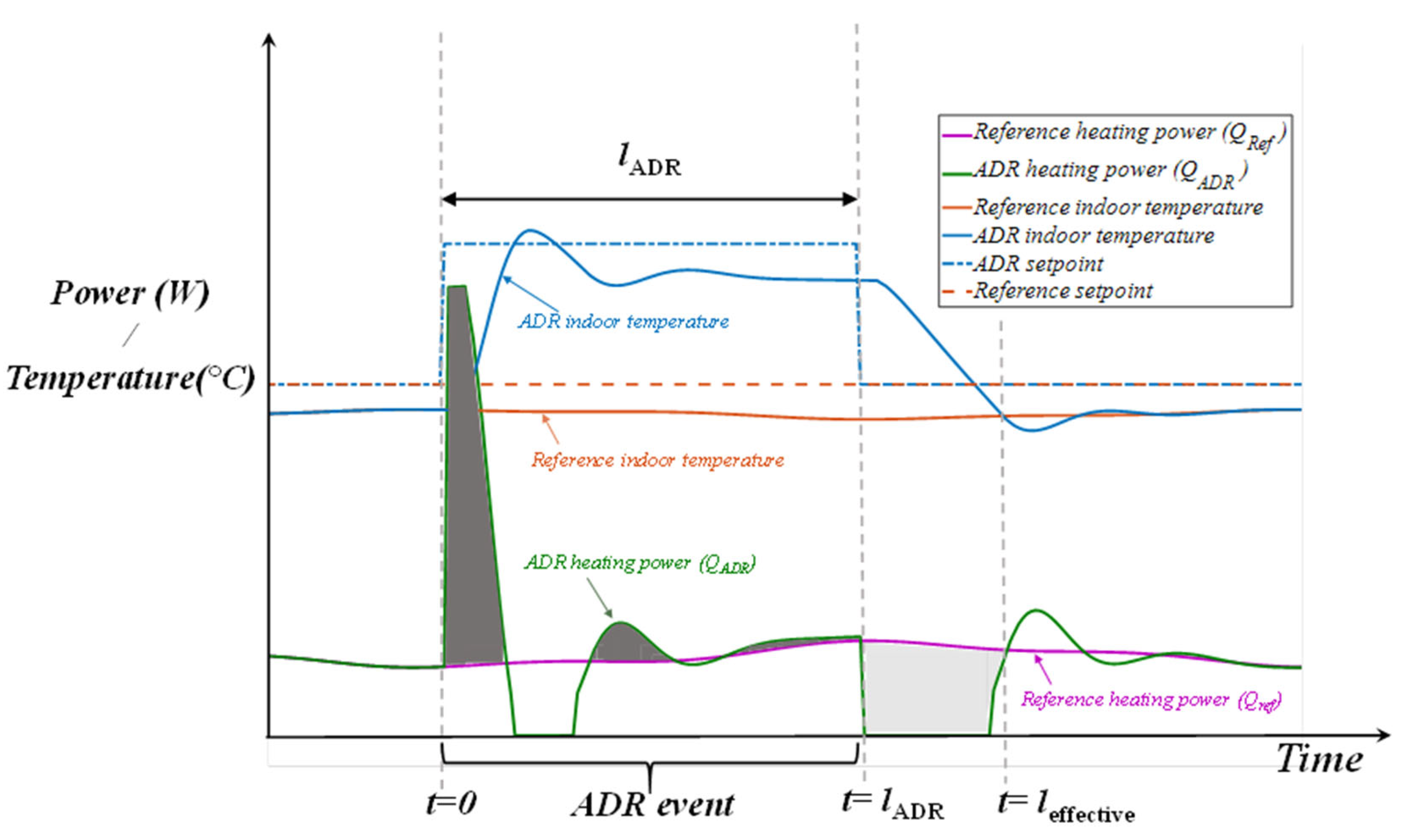
CADR is quantified by the integral of the difference between the heating power during this ADR event (
QADR) and the heating power in normal reference operation (
QRef), represented by the gray area in
Figure 1.
The parameter CADR that is used in this article calculates the building energy flexibility during a desired period which is the active demand response (ADR) event.
2. The storage efficiency (
ηADR) represents the fraction of the heat that is stored during the ADR event that can be used subsequently to reduce the heating power needed to maintain thermal comfort [
14].
Another useful index that quantifies the average power increase/reduction during a specific period of time is the dynamic building energy flexibility index (
) developed by Athienitis et al. [
26] which is defined as:
BEFI defines the amount of power variation over a fixed duration that is available from a building. This index is calculated in this article as well.
3. Methodology
The modeling approach used for this study is based on the low-order lumped-parameter thermal network models which are practical for control studies and especially model predictive control [
28,
29]. In this approach the thermal mass under consideration (radiant floor concrete slab) is discretized into a number of control volumes. Each of the discretized control volumes is represented by a node and considered to be isothermal. Each of the nodes has a lumped thermal capacitance connected to it and thermal conductances connecting it to adjacent nodes. Considering the time interval p and time step Δ
t, the general form of the explicit finite-difference model for the nodes with a lumped thermal capacitance can be stated as:
where
Ti,p represents the temperature of node “
i” at time step “
p”,
Tj,p represents temperature of node “
j” at time step “
p”,
Ci is the thermal capacitance of node “
i”,
Ri,j is the thermal resistance between nodes
i and
j, and
Qi is the heat source at node
i. The time step Δ
t is selected according to this stability criteria:
where for all the nodes
i, the summation is performed for all nodes
j connected to the node
i.
A model with fewer parameters facilitates setting up the initial conditions which is a key parameter for control studies [
28]. When the details of the construction are not known, a low-order grey-box modelling approach is practical and can be developed and calibrated by means of real time data from the building [
30]. The models must be accurate enough to provide reliable information but also flexible enough for quick and computationally efficient decision making [
31,
32] especially in reaction to electric grid’s short notices on the change in price signals.
An important part of a model for zones with radiant floor heating system is the radiative and convective heat transfers, which are inherently nonlinear processes. However, the respective heat transfer coefficients are usually linearized so that the system energy balance equations can be solved with linear algebra techniques and represented with a linear thermal network. In the case of radiant floor heating, this linearization generally introduces less error for the for long-wave radiation heat transfer (
hr) than the convection heat exchange between the radiant floor surface and room air (
hcf) [
33]. For example, in the case of radiant floor heating where usually the floor is hotter than the air and the heat flow is upward
hcf is in the order of 3 W/(m
2K) while for a cold floor and warmer air it is in the order of 1 W/(m
2K) [
33]. Therefore, usually a certain amount of calibration for the convection heat exchange between the radiant floor and room air is required for a model especially when considering the low-order models. Heat flow upwards
hcf can be calculated as [
34]:
where
Tfloor is the floor surface temperature and
Tair is the zone air temperature.
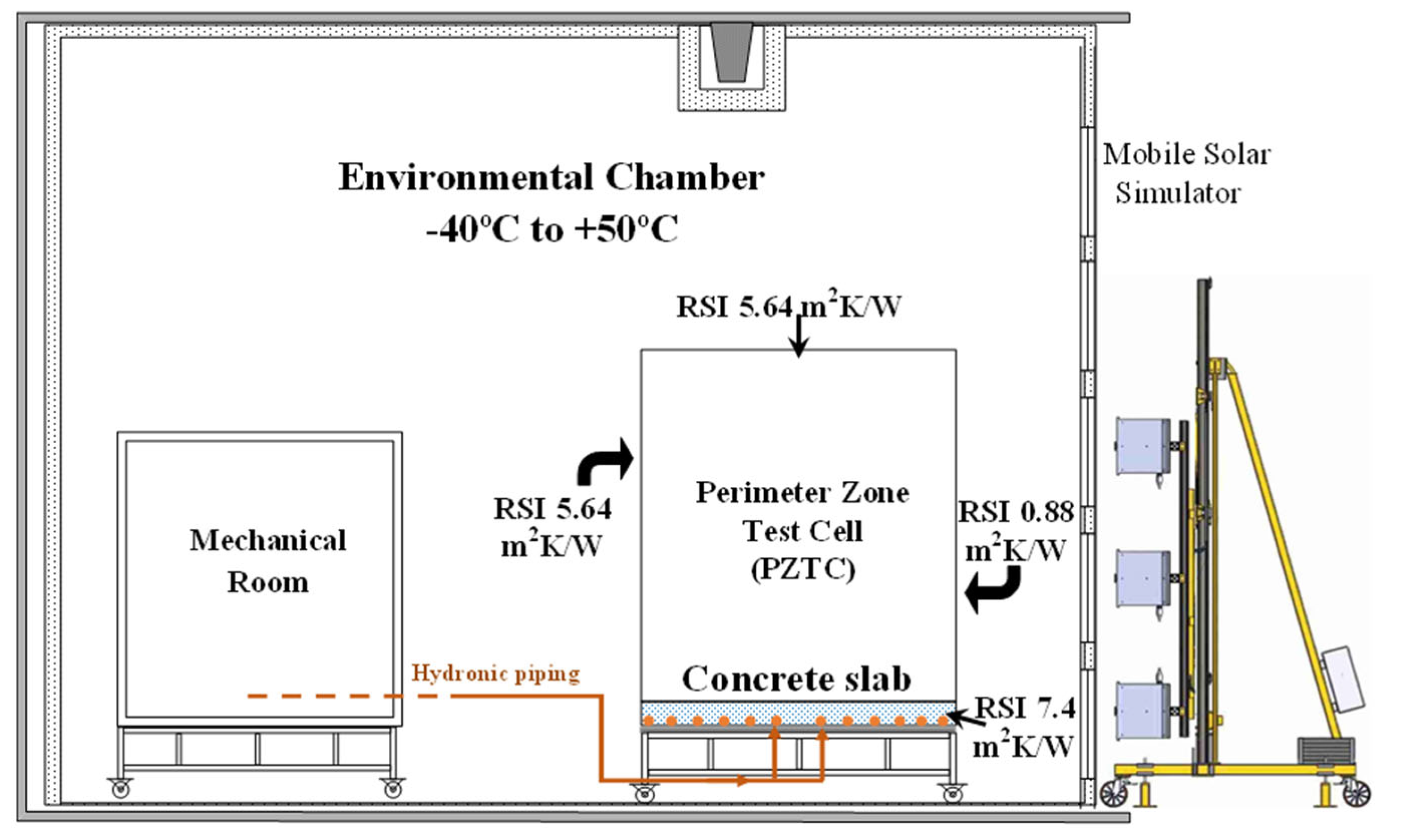
A well-calibrated low-order model can accurately capture the most important thermal dynamics of a zone with a radiant floor heating system. This modeling technique was validated through experiments in a Solar Simulator/Environmental Chamber and PZTC test facility. The Solar Simulator/Environmental Chamber (SSEC) laboratory is an experimental facility located at Concordia University in downtown Montreal, Canada. This facility allows accurate and repeatable testing of solar systems and advanced building envelopes under standard test conditions with simulated solar radiation and indoor plus outdoor conditions. The temperature test range of the environmental chamber is −40 °C to +50 °C. Two solar simulators (large-scale and mobile) are designed to emulate solar radiation to test solar systems such as PV and PV/T modules, solar air collectors, solar water collectors, and building-integrated solar systems. The perimeter zone test cell (PZTC) is a 3 m × 3 m × 3 m office placed inside the Solar Simulator/Environmental Chamber laboratory, and it has a radiant floor heating/cooling system. The side and back walls and ceiling consists of 10 cm of insulation with thermal resistance of 5.64 m
2K/W. The front wall is designed to be modifiable to test different facades and glazing systems and currently has a thin cover with 0.88 m
2K/W thermal resistance. The floor is fabricated of an approximately 8 cm thick concrete slab, with the piping at the bottom of the concrete and insulation of 7.4 m
2K/W under the slab. Thermal properties of the concrete are shown in
Table 1.
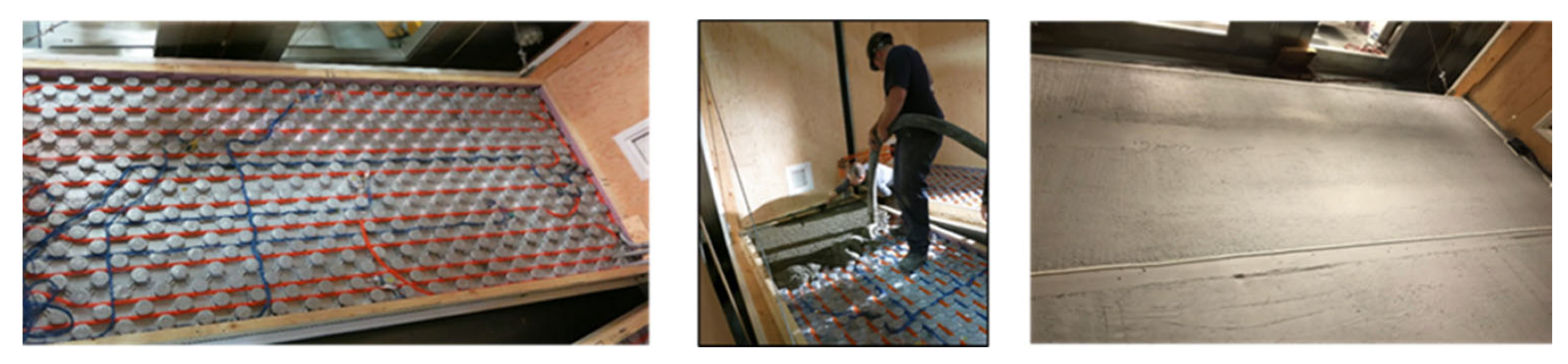
The pipes of the radiant floor system are fabricated of conventional cross-linked polyethylene (PEX) and have an external diameter of 1.75 cm. The pipes are installed in a foam matrix of insulating material that also facilitates keeping them in place. The pipes are spaced at 15 cm.
Figure 2 shows the piping configuration of the radiant floor before the concrete was poured (left), during pouring of concrete, and the final look of the radiant floor slab (right).
A mechanical room provides controlled flow rate of the fluid (propylene-glycol and water mixture) for the radiant floor. The schematic of the environmental chamber and PZTC is shown in
Figure 3.
A low-order (second-order) grey-box model was developed by the authors for the PZTC.
Figure 4 shows thermal network model of the PZTC. To study the effect of variable window to wall ratio (WWR) on energy flexibility, initially 50% WWR was considered for the front façade of the PZTC.
As mentioned before, the floor convective heat transfer can vary significantly depending on the temperature difference between the floor surface temperature and the air in the zone. Therefore, an objective function is defined to find the effective values of
hcf so that the floor surface temperature calculated from the simulations (
Tfloor, simulated) matches with experiment (
Tfloor, measured) as accurately as possible. Therefore, the objective function is defined using the Euclidean norm of the difference as:
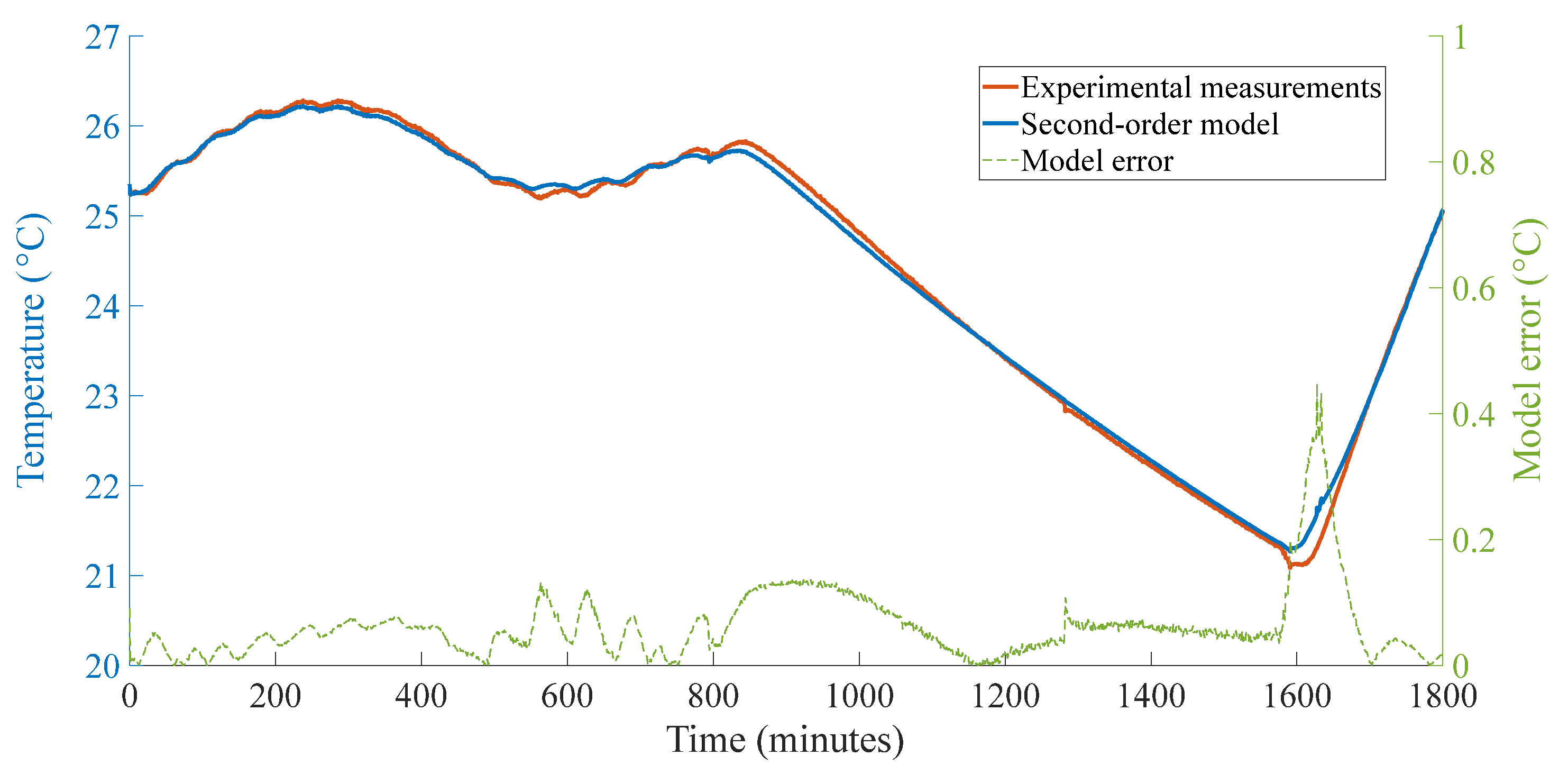
Optimization was performed in MATLAB using the fmincon function which uses the simplex algorithm. The optimization result is shown in
Figure 5.
As observed, a well-calibrated low-order model can capture thermal dynamics of a zone that contains radiant floor heating system with a good accuracy and the maximum error between the model and the measurements is about 0.45 °C. However, for the majority of the time the model error is less than 0.1 °C. Moreover, another fitness metric is the coefficient of variance of the root mean square error (CV-RMSE) shown in Equation (8) in which
Ti is the measured temperature and
is the simulation temperature,
n shows the total number of observation and
is the average of all measurements.
According to ASHRAE Guideline 14 [
35], a model should not exceed a
CV-RMSE of 30%. The
CV-RMSE is calculated here to be 15%.
The validated low-order model is used in the following section to study different control strategies based on the floor surface temperature, zone air temperature, and operative temperature. The quantified energy flexibility for each case is compared with each other. An external façade with 50% WWR double-glazed, low-e windows was considered for the PZTC. The heating is controlled by the proportional control strategy which is defined as:
where
Kp is the proportional constant,
Tsp is the desired setpoint temperature and
Tcontrol is the controlled temperature which here is the floor surface (
Tfloor), air (
Tair), and operative (
Top) temperatures, respectively.
4. Results
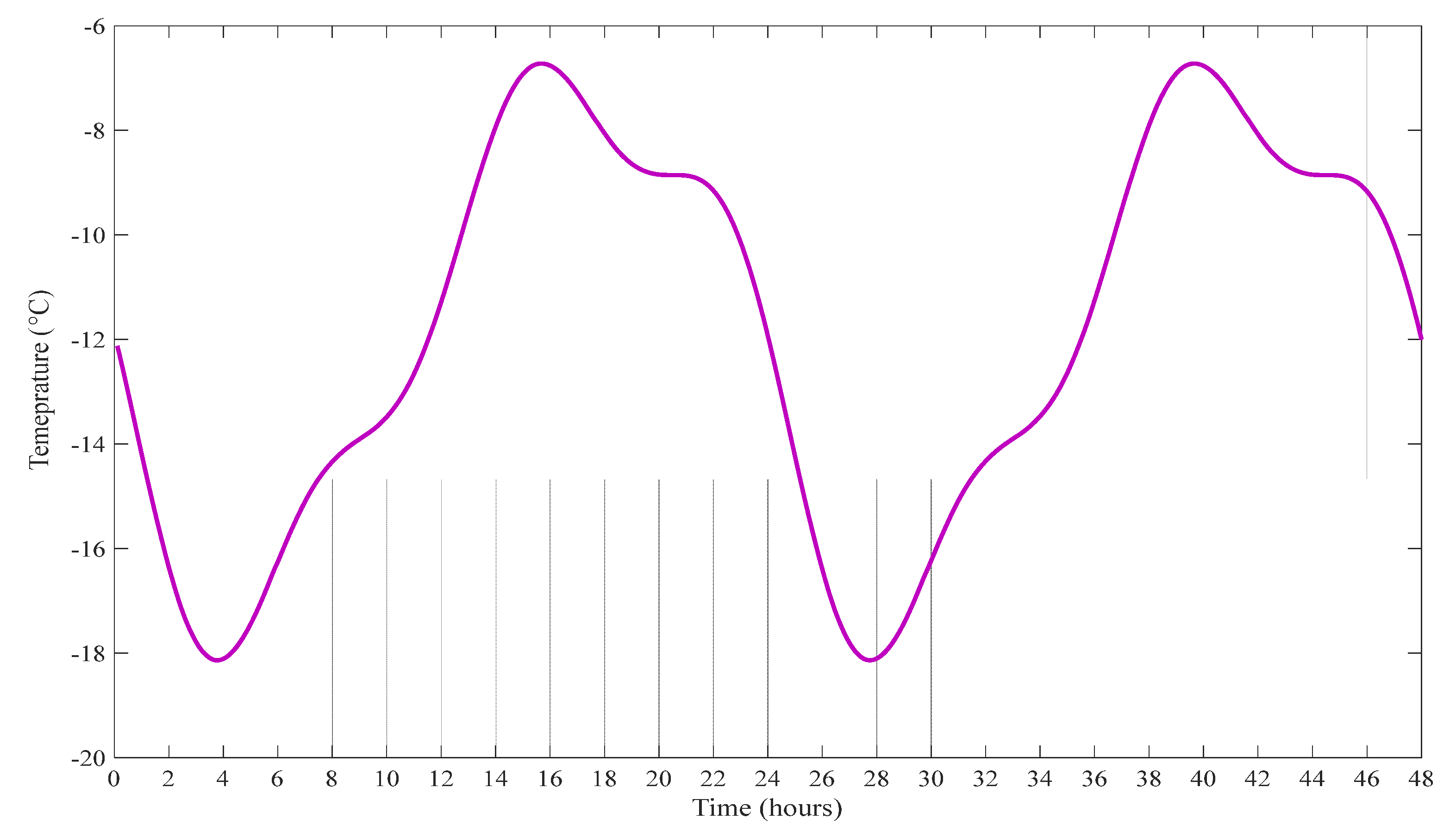
This section presents the simulation results of controlling different temperatures in the thermal zone and their respective energy flexibility by means of the validated second-order model. The outdoor condition is considered as a cloudy cold winter day in Montreal as shown in
Figure 6. The goal here is to evaluate and quantify the downward and upward energy flexibility for the evening and morning peak demand periods respectively for a typical cold winter day. Therefore, in order to let the model stabilize from the initial conditions, two identical days (48 h) were considered for simulations first.
Next section presents results of floor surface temperature control starting from the reference setpoint profile and then showing the results for the downward and upward flexibility strategies.
4.1. Floor Surface Temperature Control
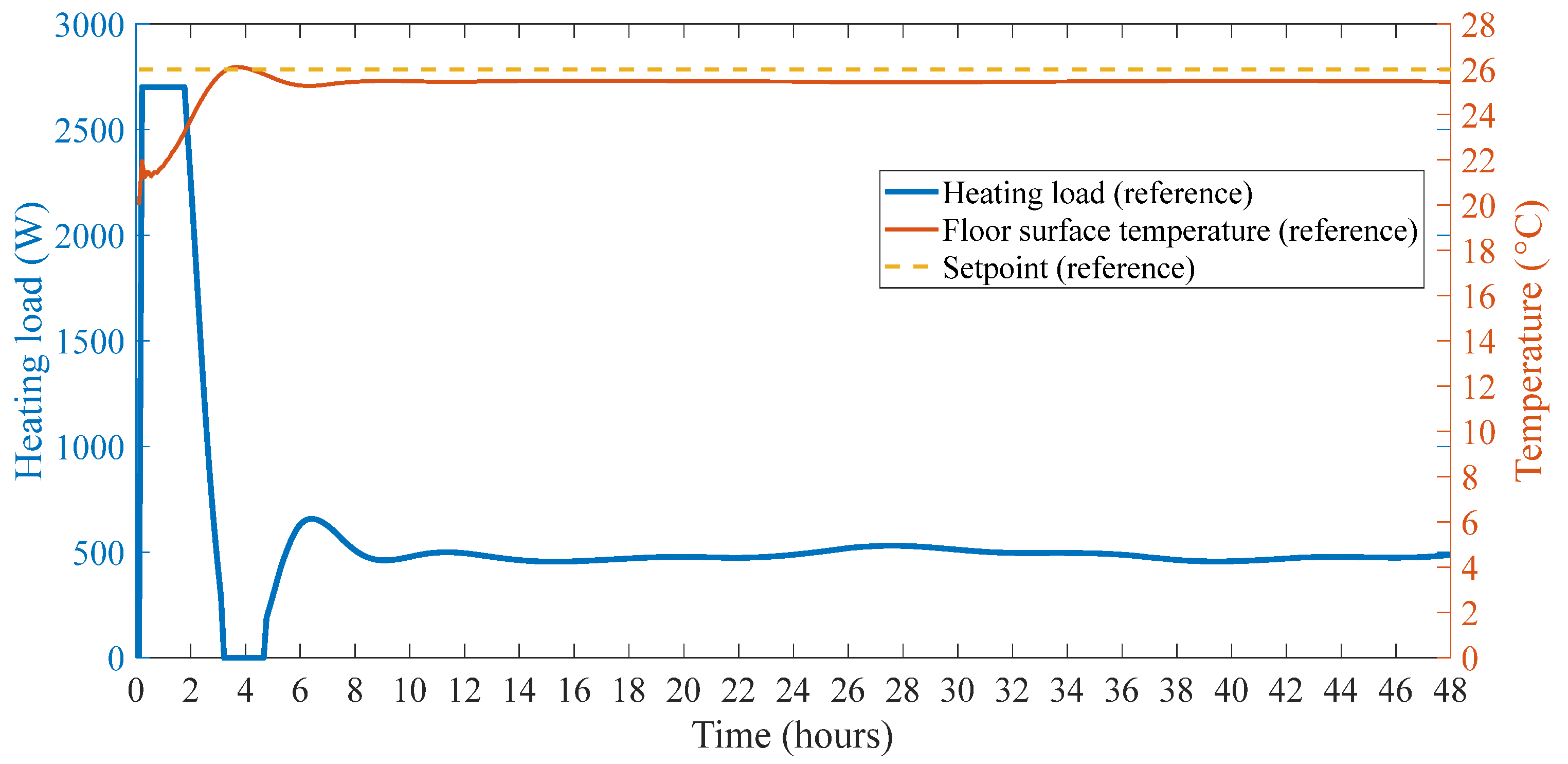
Figure 7 shows the heating load profile for the floor surface temperature control considering the constant, reference setpoint of 26 °C. It can be observed that the heating load changes during this 48-h period and a relatively smooth load profile is seen.
Considering that a higher than usual penalty signal from the grid is observed on the first day during the evening peak demand period, which is around 4 to 8 p.m., if we perform the reactive control and lower the surface temperature setpoint by 2 °C (from 26 °C to 24 °C) during that period, the following change in the heating load is observed and shown in
Figure 8:
As observed, by lowering the setpoint, the heating load drops to zero due to the thermal mass of the concrete slab. For this 4 h period, the downward flexibility, CADR,D is calculated from Equation (1) and is equal to 198 Wh/m2.
With this control strategy, the zone air and operative temperatures stay within the comfort range as observed in
Figure 9.
The
BEFID for this downward flexibility event is 457 W or
BEFID = 50 W/m
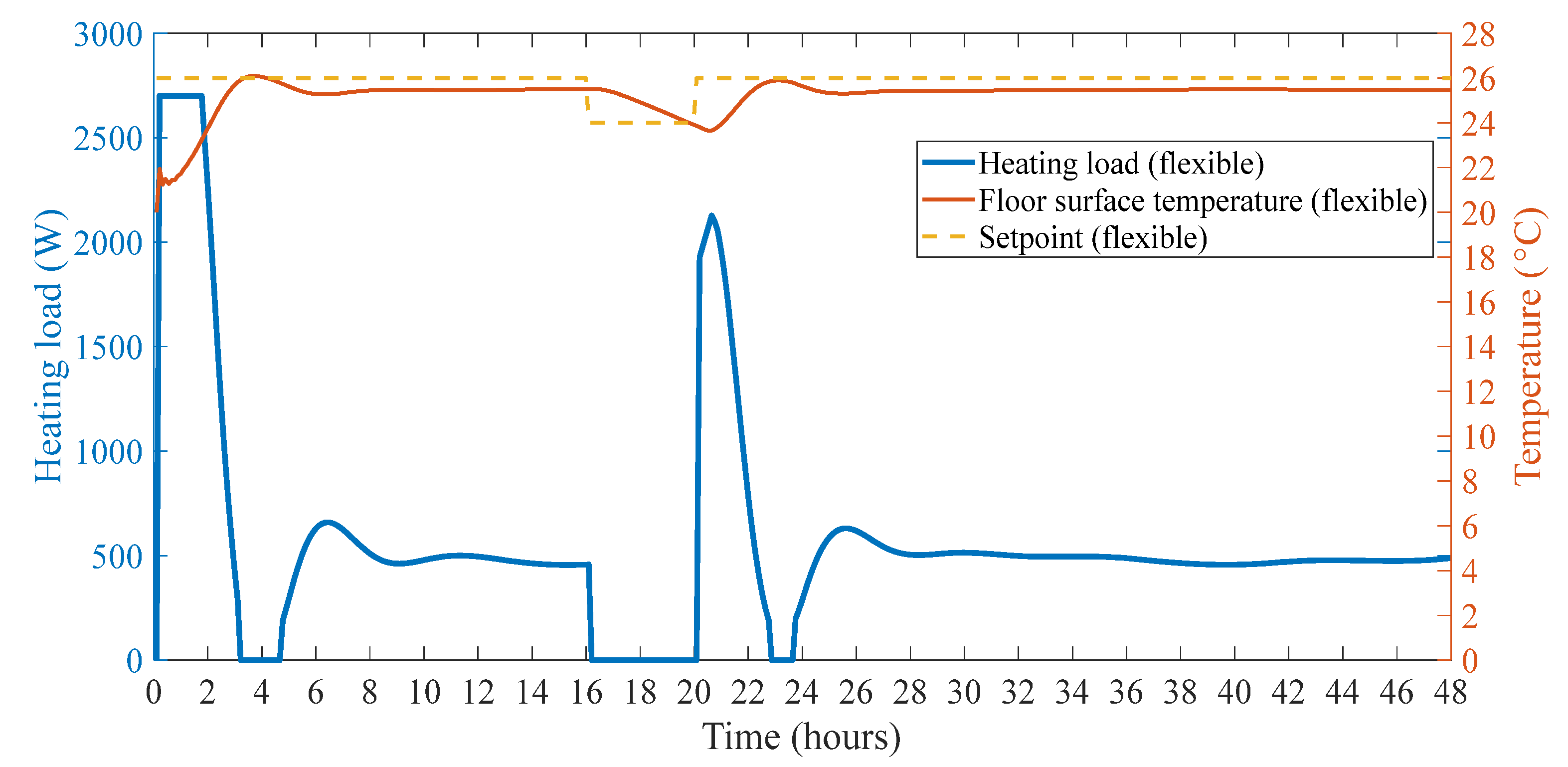
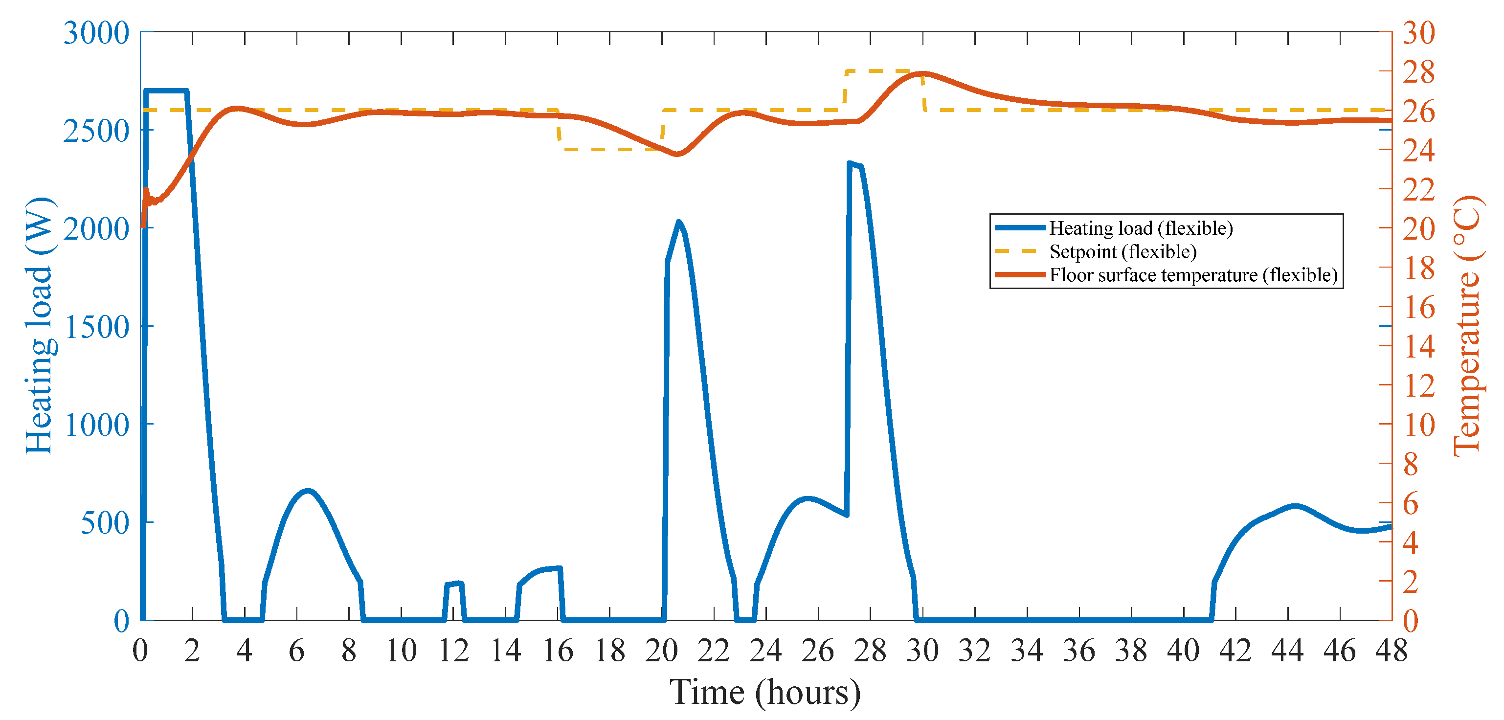
2. For the next day, the morning peak period of 6–9 a.m. (hours 30–33 in the figure), a predictive strategy is considered to preheat the slab by increasing the setpoint to 28 °C at night for 3 h (from 27 to 30) just before the morning peak demand period. As observed in
Figure 10, then the heating load and energy consumption is zero during the peak demand period and even one hour after that (4 h in total). The upward flexibility for this 3 h period is calculated as
CADR,U = 222 Wh/m
2 and the
BEFIU = 76 W/m
2.
The storage efficiency for the rest of the day is calculated as ηADR = 91%. This means that for the rest of the day, 91% of the stored thermal energy during the morning ADR event, equal to 202 Wh/m2, is used to further change and decrease the heating load during the rest of the day compared with the reference case.
4.2. Air Temperature Control
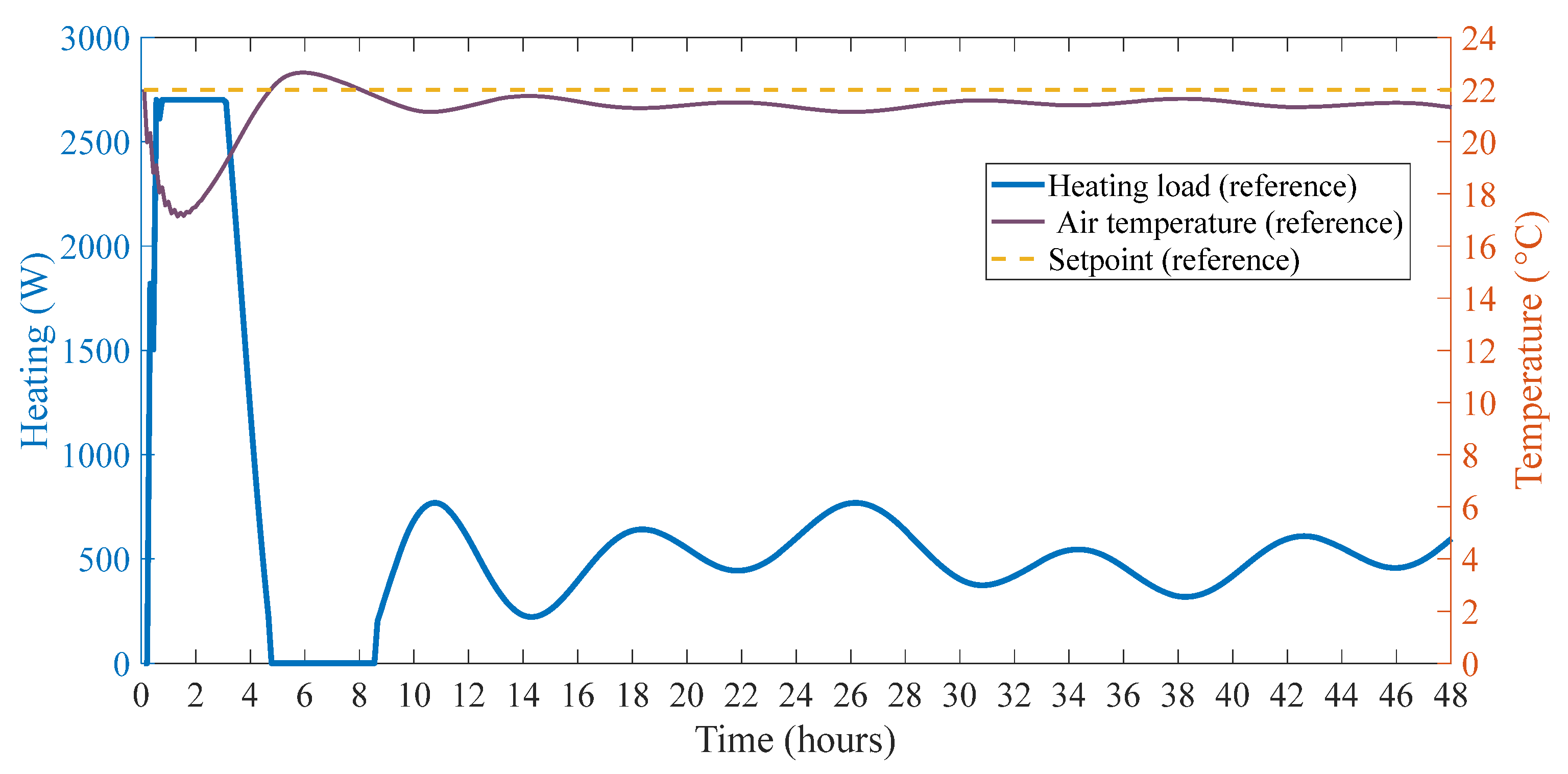
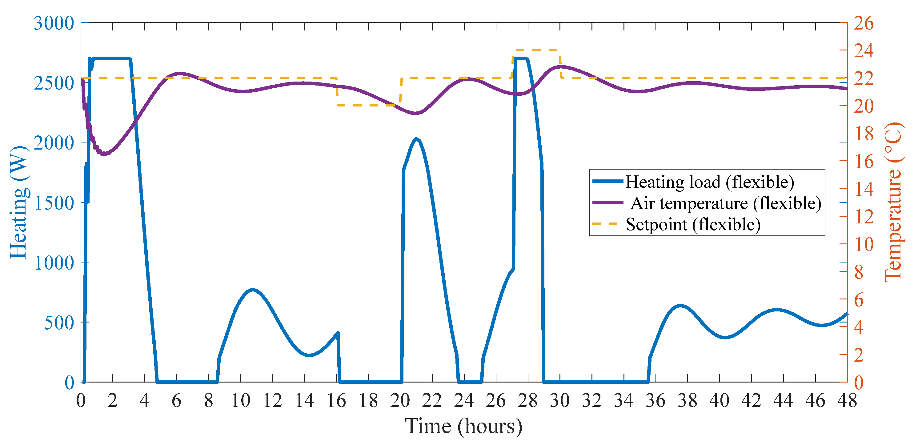
If we consider the zone air temperature control instead of the floor surface, the heating load profile for the reference setpoint of 22 °C is shown in
Figure 11.
Comparing
Figure 10 and
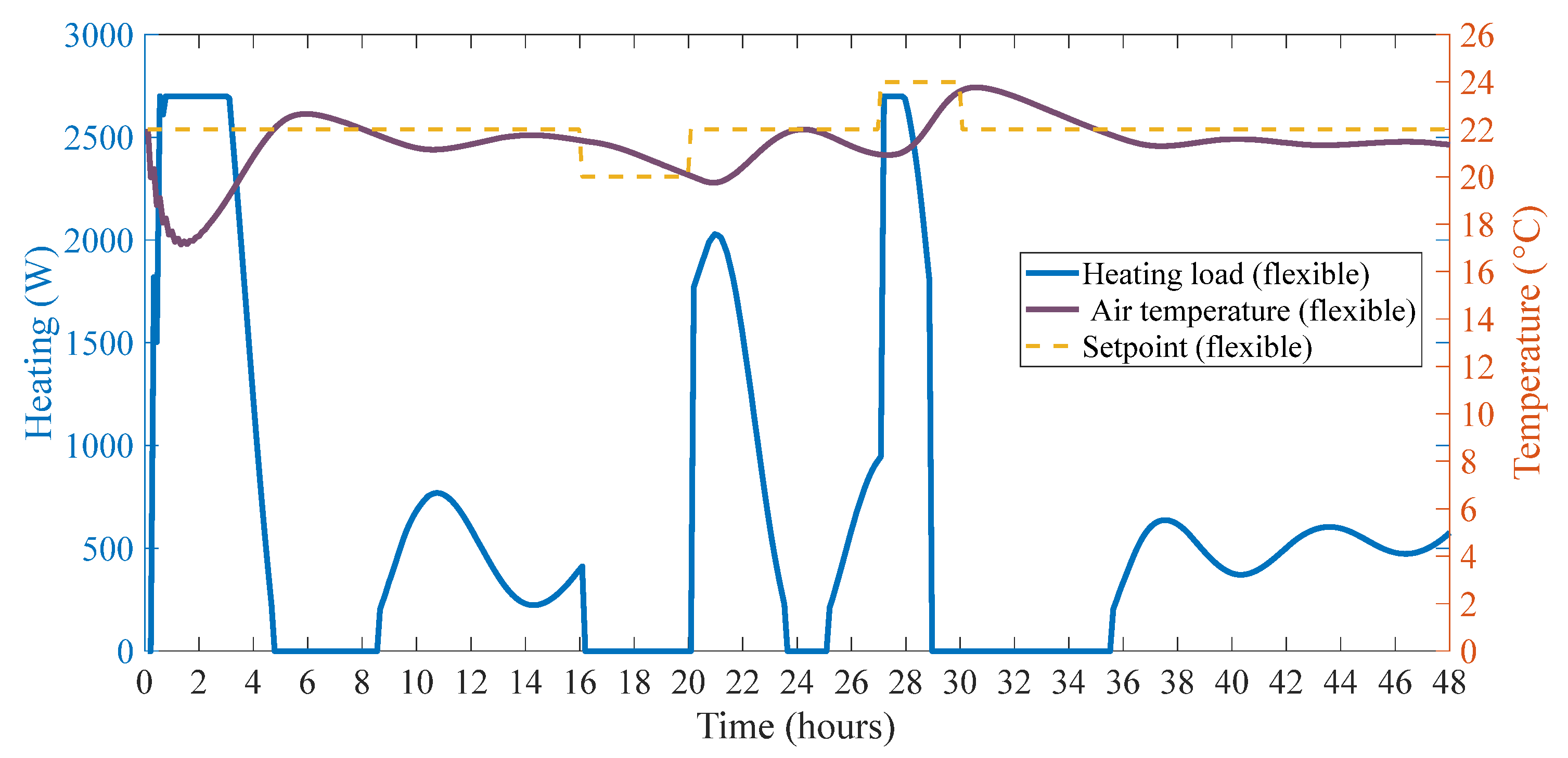
Figure 11, we can see more fluctuations in the heating load profile for the air temperature control compared with the floor surface which is due to the much lower thermal mass of zone air compared with the concrete slab. Now, applying the same strategy, If the air temperature setpoint is decreased by 2 °C (to 20 °C) during the first day evening peak demand period (hours 16–20),
Figure 12 shows the heating load profile.
For this case, CADR,D for the 4 h period is equal to 247 Wh/m2 which considering the same 2 °C drop in the setpoint, shows about a 25% increase compared with the previous case of floor surface temperature control (194 Wh/m2). Furthermore, the average reduction in heating power is equal to: BEFID = 63 W/m2.
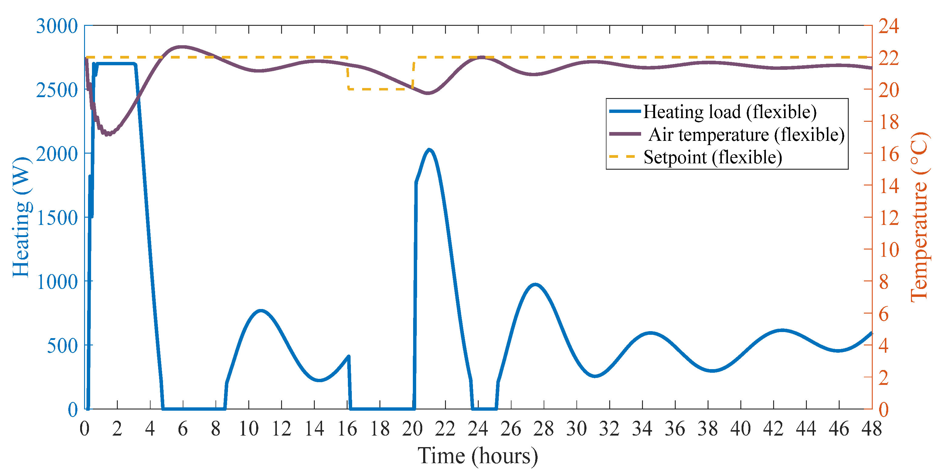
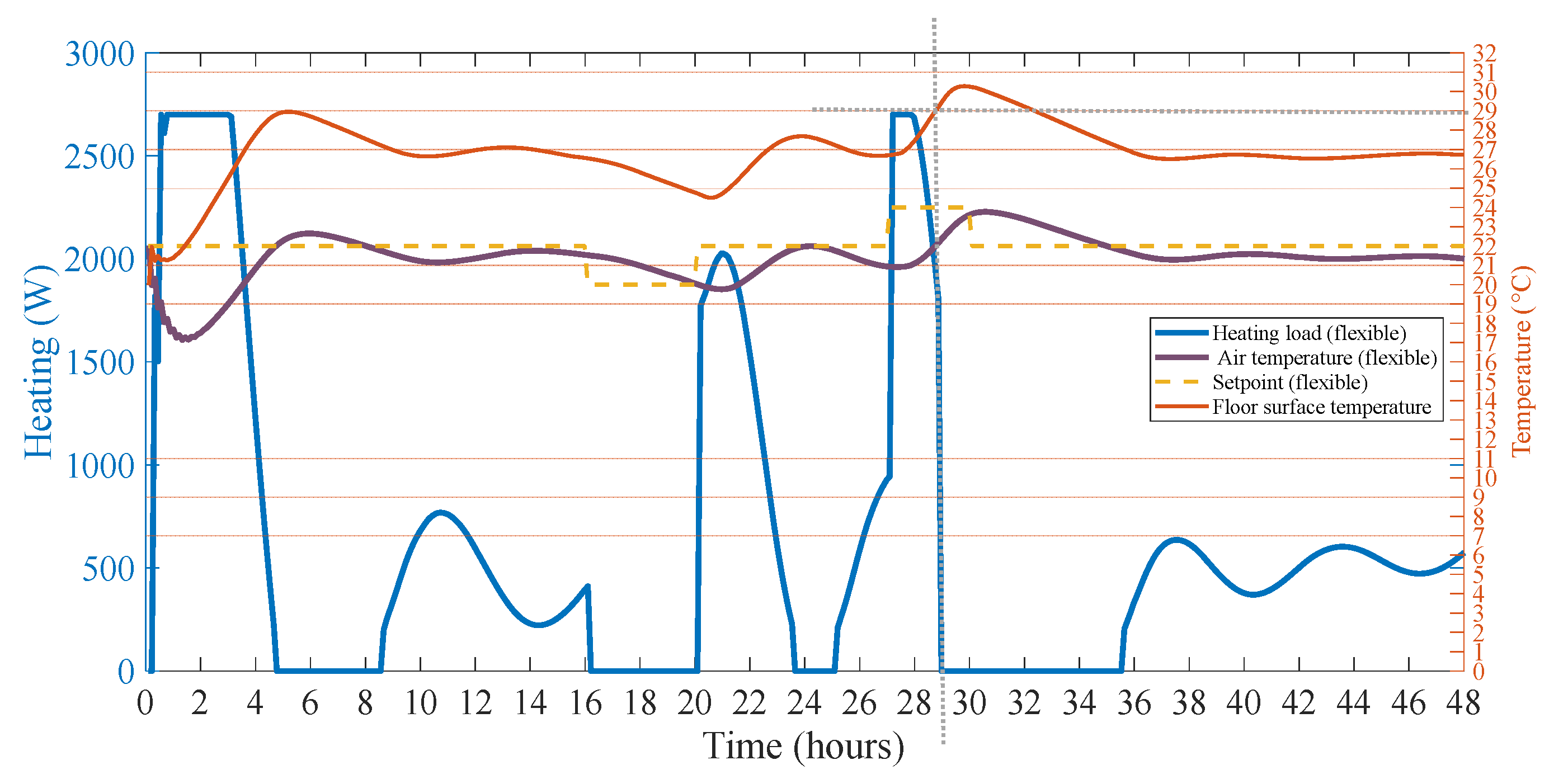
Considering the preheating before the next day’s morning peak period (hours 30–33), the heating profile is shown in
Figure 13. The upward flexibility for this case is calculated as
CADR,U = 313 Wh/m
2 which is 40% higher compared with the case of floor surface temperature control (222 Wh/m
2).
It is observed that this control strategy based on zone air temperature also results in 5.5 h of zero heating load after the upward flexibility event compared with the 4 h with floor surface temperature control. The storage efficiency for the rest of the day is calculated as ηADR = 78%, meaning that after the morning ADR event, 313 × 0.78 = 244 Wh/m2 is used to further reduce the heating load for the rest of the day. The average increase in heating power during this ADR event is equal to BEFIU = 104 W/m2 which shows about a 37% increase compared with the previous case with floor surface temperature control.
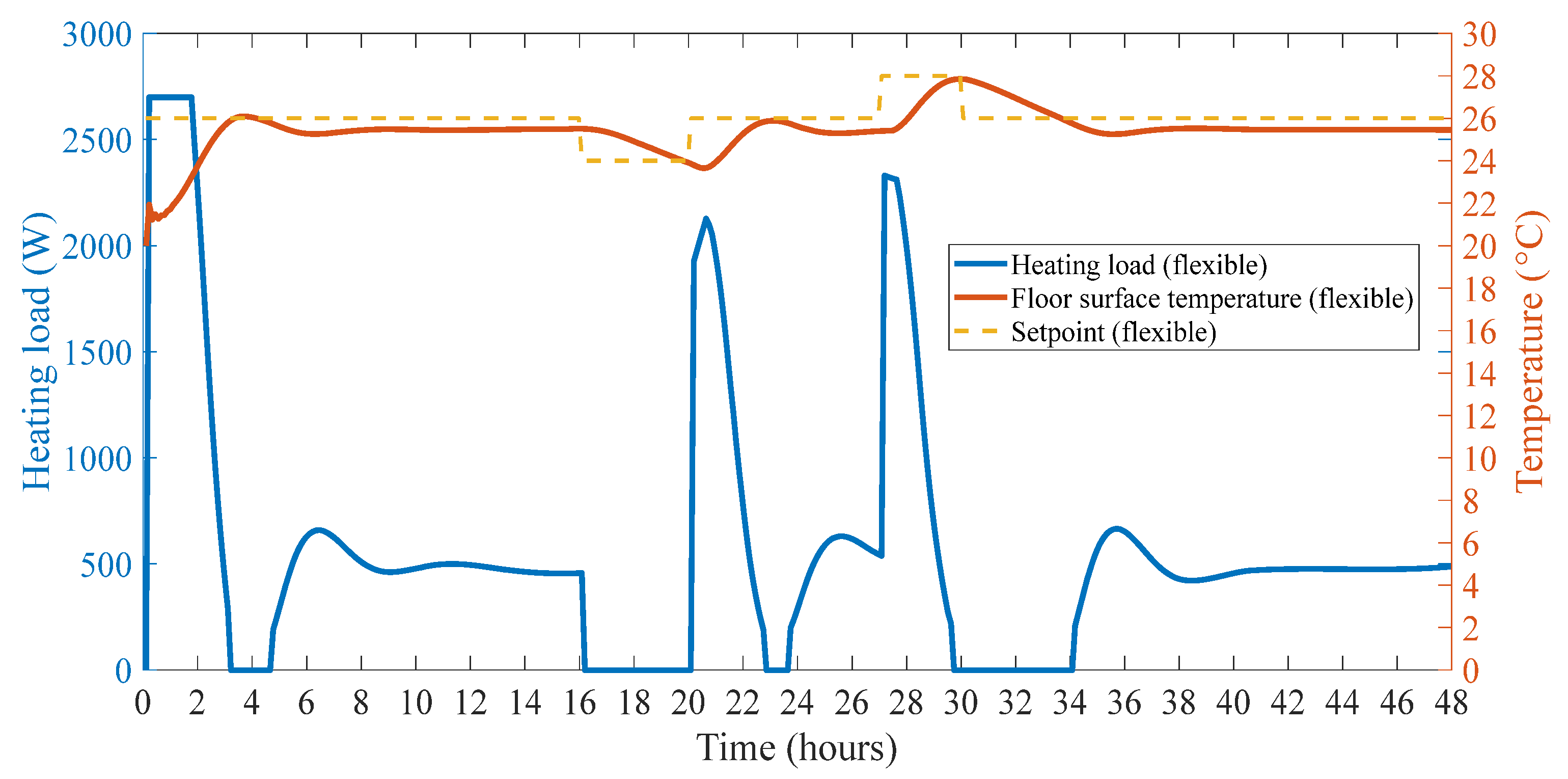
Another important observation in
Figure 13 is that during the upward ADR event, the heating load is stopped around hour 29 while the air temperature did not reach the threshold of 22 °C. The reason for this is that in the radiant heating system, there is a limitation for the floor surface temperature to not exceed 29 °C based on the ASHRAE standard [
35]. Therefore, as seen in
Figure 14, when the floor surface reaches 29 °C, the heating is stopped automatically.
4.3. Operative Temperature Control
Based on ASHRAE standard 55, the operative temperature of a zone is defined as [
35]:
where
Tmr is the mean radiant temperature and
Tair is the zone air temperature.
For the operative temperature control,
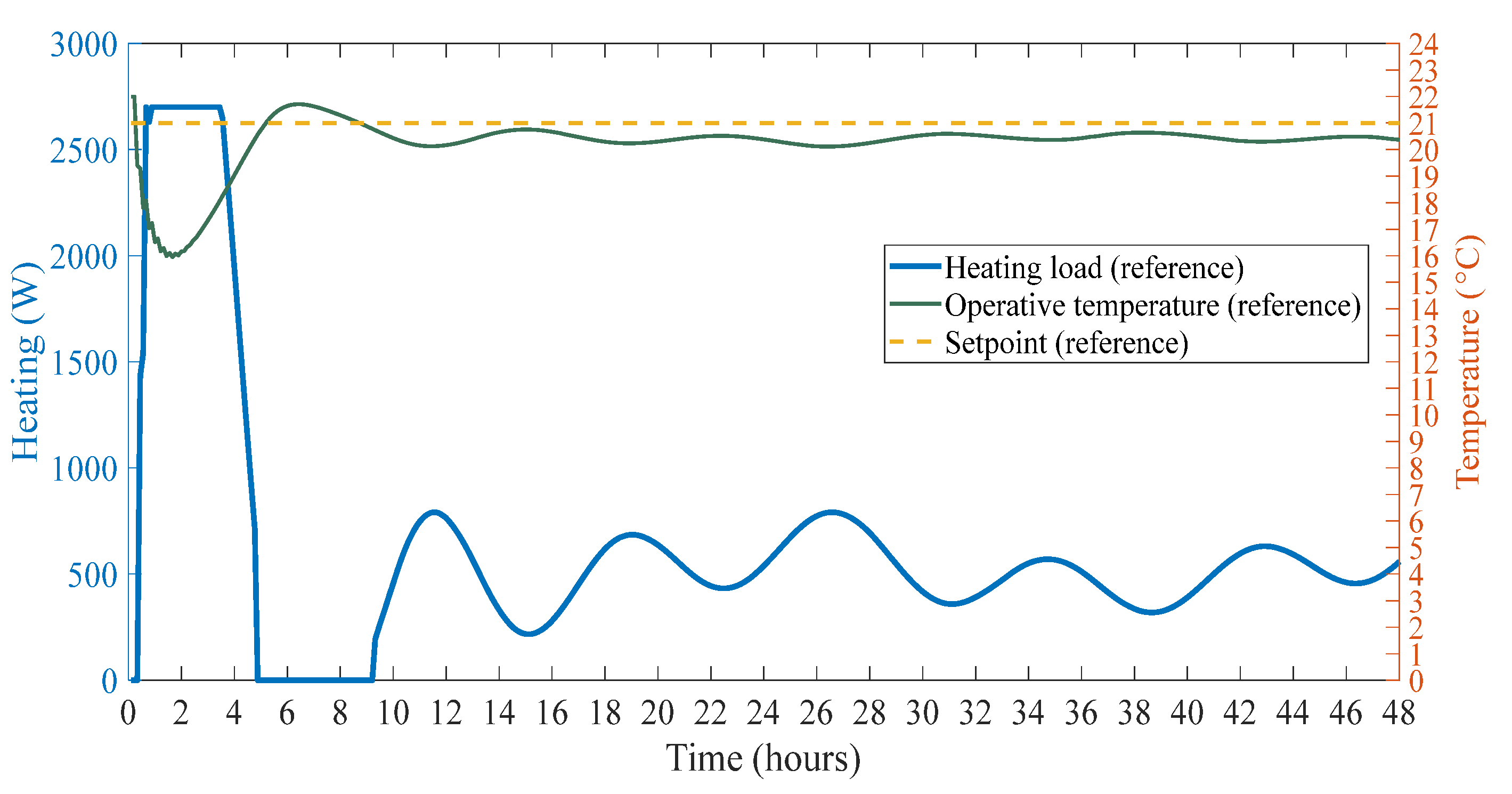
Figure 15 shows the heating load profile for the reference setpoint of 21 °C.
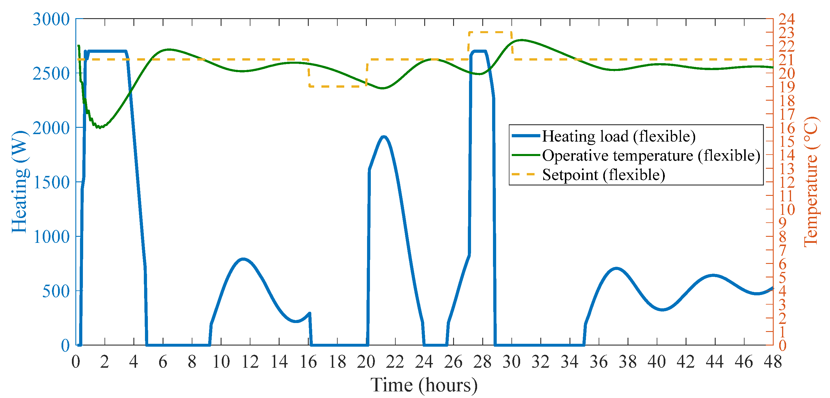
Similar to the previous cases, for the downward and upward flexible case, the heating load is shown in
Figure 16.
For the downward flexible case, CADR,D = 240 Wh/m2 and BEFID = 61 W/m2; and for the upward flexible case, CADR,U = 294 Wh/m2, and BEFIU = 97 W/m2. The storage efficiency for the rest of the day is calculated as ηADR = 73%.
Table 2 sums up the results for different cases and control strategies.
Comparing the three cases, it is observed that for the same reduction or increase of 2 °C in the corresponding setpoint, the air temperature control strategy results in higher CADR and BEFI and therefore higher energy flexibility (both upward and downward) as well as longer hours of zero load compared with floor surface and operative temperature control.
4.4. Effect of Increasing the WWR
The effect of increasing the window area of the exterior façade on the energy flexibility was investigated. The WWR increased from 50% to 75%.
Figure 17 shows the comparison of the two variations for the reference case of air temperature control.
As expected, there is a noticeable increase in the heating load.
Considering the flexible setpoint, the heating load for the 75% WWR is shown in
Figure 18.
The downward and upward energy flexibilities for this case are: CADR,D = 289 Wh/m2 and CADR,U = 182 Wh/m2. Therefore, as the heating load is increased with increasing WWR, the downward flexibility is increased by 17%. However, in the case of upward flexibility, a decrease of 42% (from 313 Wh/m2) was observed.
4.5. Effect of Solar Gains
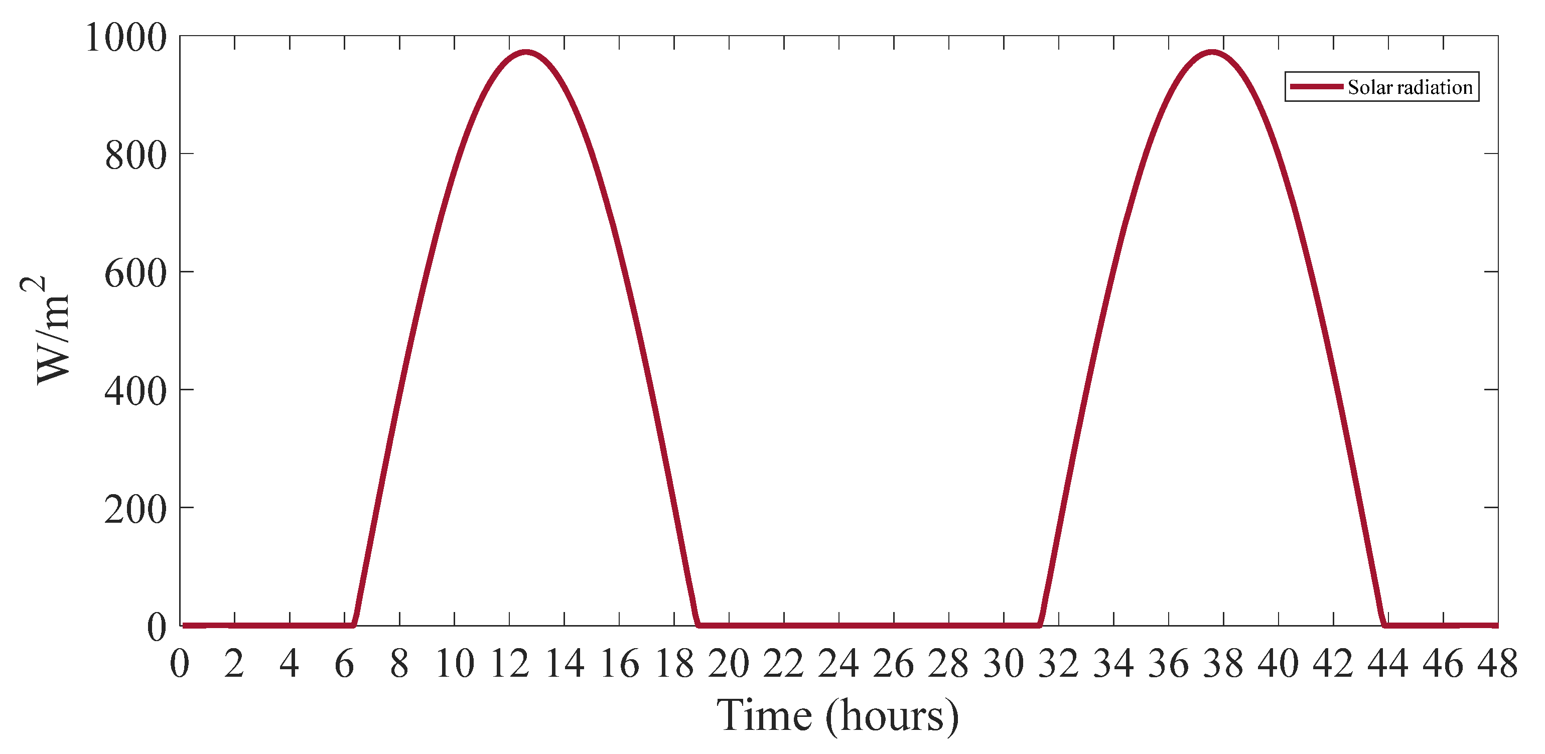
The previous section simulations were performed considering a cloudy day. Having solar gains through a part of the window on a part of the floor can have a noticeable impact on the heating load and indoor temperature and cause significant fluctuations. To evaluate this impact, a half sinusoidal solar radiation profile shown in
Figure 19 was considered and it is assumed that only a small portion of it passes through part of the window and heats part of the floor.
Figure 20 shows the reference profile for floor surface temperature control for this case.
As observed, there are more fluctuations in the floor surface temperature and the heating load profile which shows a significant impact of the solar gain. We can see that for the hours between 9 and 14.5 and for the next day between the hours 33.5 and 39.5, very little heating is required.
For the flexible setpoint case,
Figure 21 shows the load profile for the downward and upward flexibility.
For the downward flexibility case, CADR,D = 185 Wh/m2 which is 6.5% less compared with the cloudy day (198 Wh/m2) since the heating load is also smaller. Moreover BEFID = 47 W/m2, which is also 6% lower than the one for the cloudy day (50 W/m2).
For the upward flexibility, CADR,U = 231 Wh/m2 which is slightly higher (4%) than the cloudy day (222 Wh/m2) and the storage efficiency for the rest of the day is ηADR = 88%. Furthermore, the average increase in power BEFID = 76 W/m2 which is the same as the cloudy day.
As the above analysis showed, there is no major difference between the flexibility indicators and the difference is less than 7% between a cloudy and a sunny day. However, a major difference is observed during the hours of the zero heating load after the upward flexibility event. As shown in
Figure 21, about 11 h (30–41) of zero heating load is achieved with the aid of solar gains. The use of solar gains should be considered with careful considerations of shades as it can seriously fluctuate the indoor temperature and consequently the occupant comfort.
5. Discussion and Conclusions
This study presented a comparative analysis of energy flexibility for different control strategies for zones with radiant floor heating systems with significant thermal mass. It was observed that with every control strategy, a noticeable amount of energy flexibility is achieved by decreasing or increasing the control temperature setpoint during or before the high price signal (peak demand) period. For the control strategy based on the floor surface temperature, downward flexibility of CADR,D = 198 Wh/m2 and the average power reduction in BEFID = 50 W/m2 was achieved during the evening peak demand period. The upward flexibility for this case was CADR,U = 222 Wh/m2 for the 3 h before the morning peak demand period, and the average increase in BEFIU = 76 W/m2 in power was observed. The storage efficiency of ηADR = 91% was obtained for the rest of the day after the upward flexibility event, meaning about 202 Wh/m2 was used subsequently to reduce the heating load.
For the control strategy based on the air temperature control, the calculated variables were CADR,D = 247 Wh/m2 and BEFID = 63 W/m2 for the downward case, and CADR,U = 313 Wh/m2 and BEFIU = 104 W/m2 for the upward case. The storage efficiency for this case was ηADR = 78% for the rest of the day after the upward flexibility event, meaning about 244 Wh/m2 was used subsequently to reduce the heating load.
For the control strategy based on the zone operative temperature control, the calculated variables were CADR,D = 240 Wh/m2 and BEFID = 61 W/m2 for the downward case and CADR,U = 297 Wh/m2 and BEFIU = 97 W/m2 for the upward case. The storage efficiency for this case was ηADR = 73% for the rest of the day after the upward flexibility event, meaning about 216 Wh/m2 was used subsequently to reduce the heating load.
Therefore, it was observed that the control strategy based on air temperature results in a significantly higher energy flexibility compared with the floor surface temperature or operative temperature control. For the downward flexibility, with air temperature control there was a 20% increase compared with the floor surface temperature, and for the upward case an increase of 30% was observed. This is an important consideration in the design of control strategies for the zones with radiant floor system where higher energy flexibility is a major objective.
It was observed that increasing the window to wall ratio (WWR) results in 17% increase in the downward flexibility which is due to the general increase in the reference heating load when the WWR was increased. Moreover, a 42% decrease in upward flexibility was observed.
The effect of solar gains was also investigated, and it was observed that for the case of floor surface temperature control strategy, a 6.5% decrease in downward flexibility and 4% increase in the upward flexibility were observed. The major difference for this case is utilizing the solar gains during the day for a significant increase in the zero load hours which is about 11 h compared with 4 h for the cloudy day.
For future work, it is suggested to perform experimental studies for implementation in large buildings equipped with high-mass radiant systems which can perform both radiant heating and cooling.


