
Artificial Neural Network for Predicting Building Energy Performance: A Surrogate Energy Retrofits Decision Support Framework


Abstract
:1. Introduction
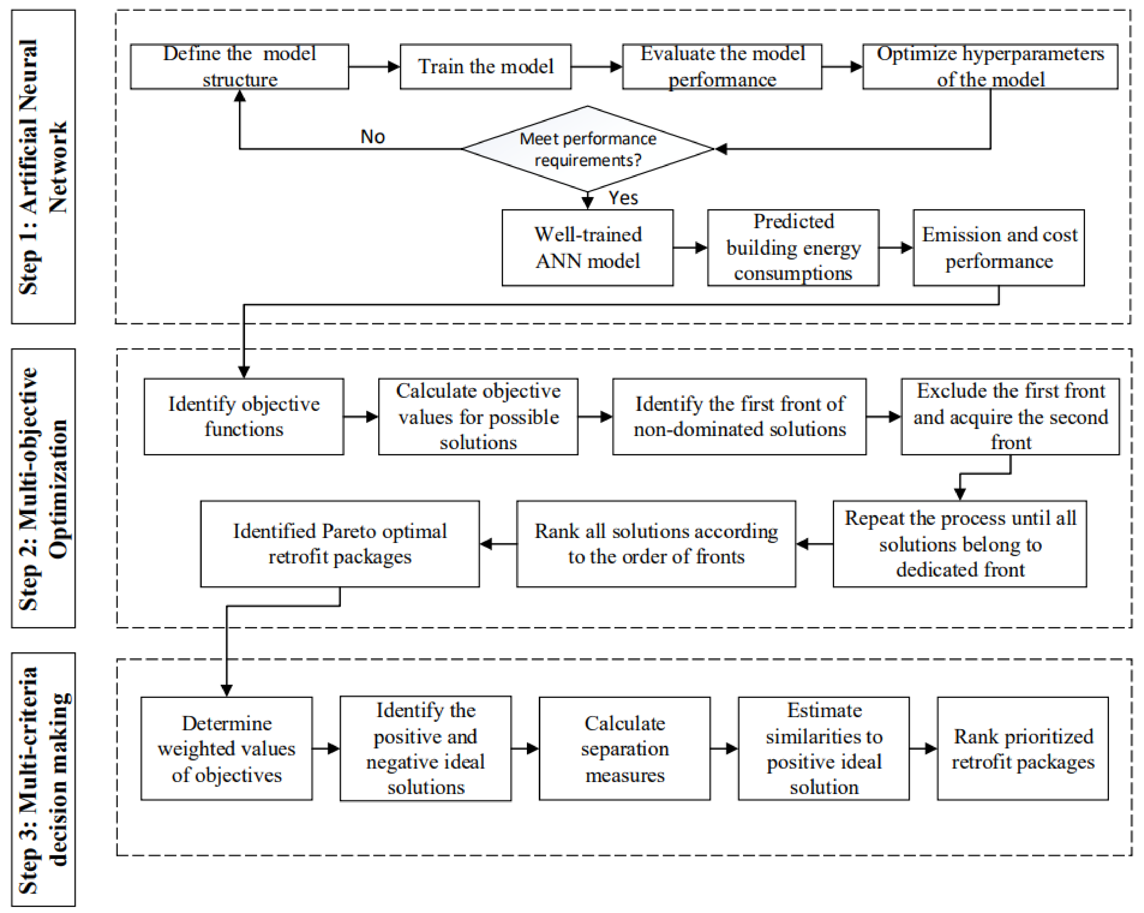
2. Methodology
2.1. Artificial Neural Network
2.1.1. Data Collection and Preparation
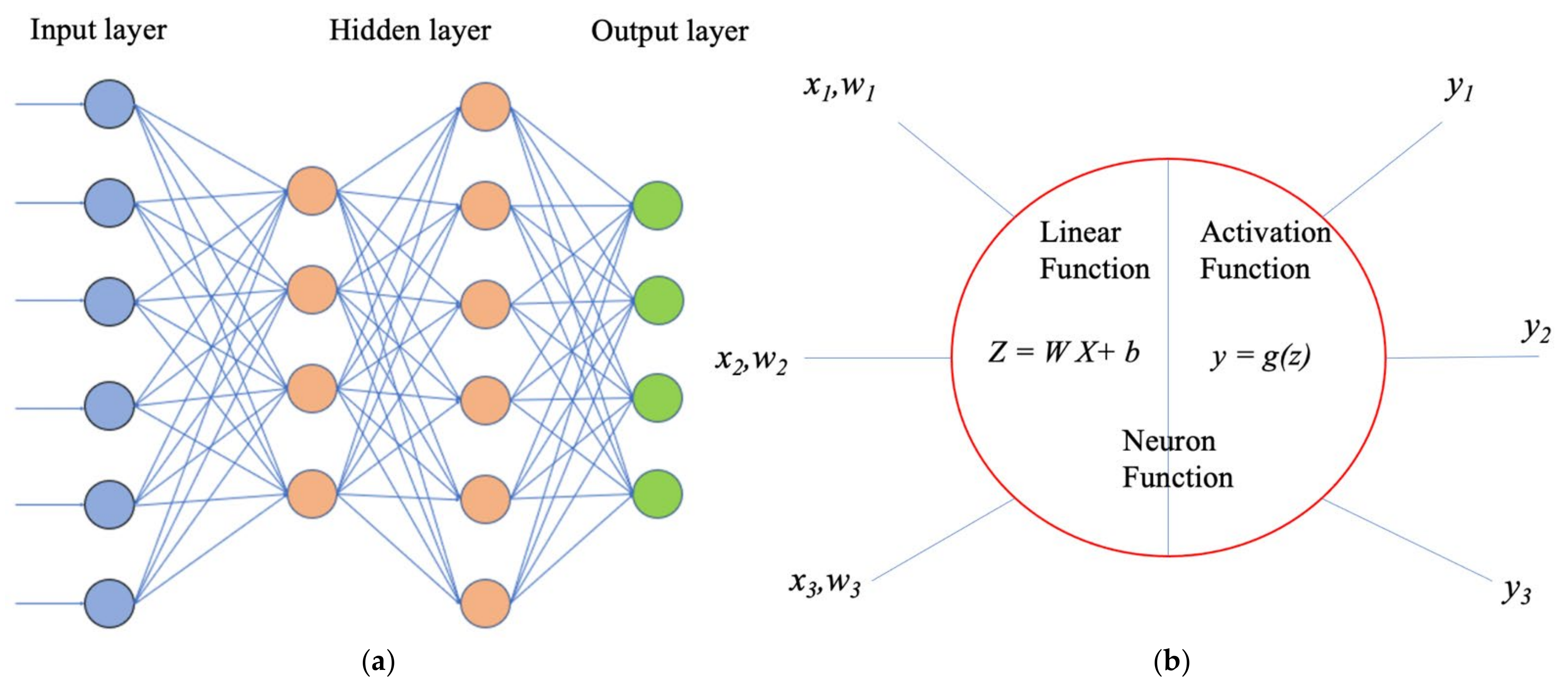
2.1.2. Model Development
- Inputs : The input features of the ANN model.
- Weights : The parameter that needs to be identified by training the model.
- Bias : The parameter that needs to be identified by training the model.
- Activation function : The function of a neuron that defines the outputs of that neuron given a set of inputs.
- Outputs : The output variables of the ANN model.
2.1.3. Model Performance Evaluation
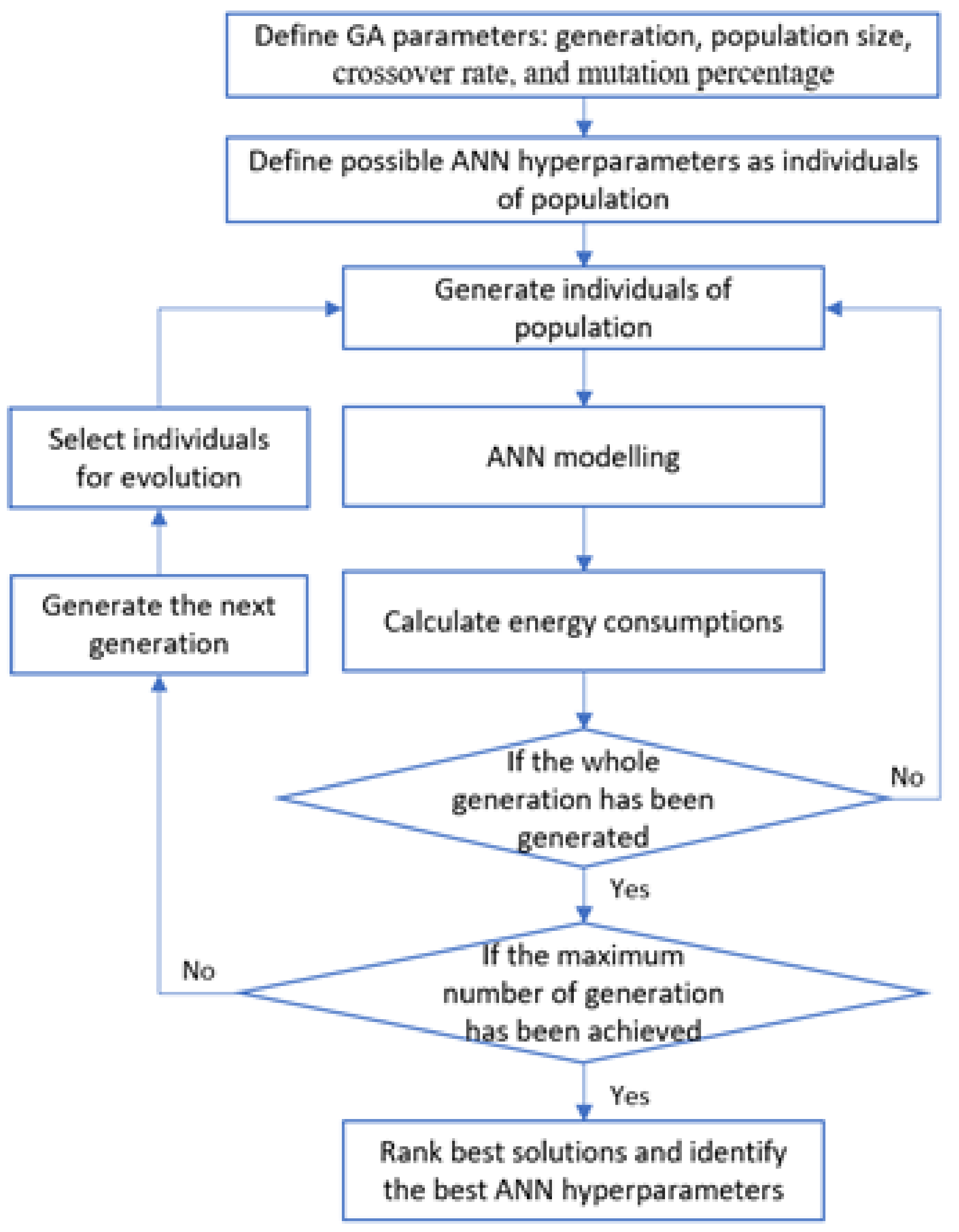
2.1.4. Optimization of Hyperparameters
2.2. Multi-Objective Optimization
2.2.1. Objective Functions
Retrofit Emissions
- = The carbon emission of the base building model by taking the candidate solution (kg CO2e).
- = The electricity consumption of the building model by employing the candidate solution (kWh).
- = The natural gas energy consumption of the building model by taking the candidate solution (GJ).
- = Local electricity grid emission factor (kg CO2e/kWh).
- = Natural gas emission factor (kg CO2e/GJ).
- = The remaining lifetime of the retrofitted building.
Retrofit Costs
- = The initial retrofit cost of the candidate retrofit solution.
- = The initial costs of envelope component materials.
- = The initial costs of energy equipment.
- = The unit initial cost of the insulation material.
- = The initial cost of the energy equipment.
- = The annual operational cost savings by taking the candidate retrofit solution.
- = The local electricity price (CAD/kWh).
- = The local natural gas price (CAD/GJ).
- = The annual maintenance cost.
- = The net present value of operational energy cost savings.
- = The discounted rate (%).
- = The retrofit project lifetime.
- = The life cycle cost of the candidate retrofit solution.
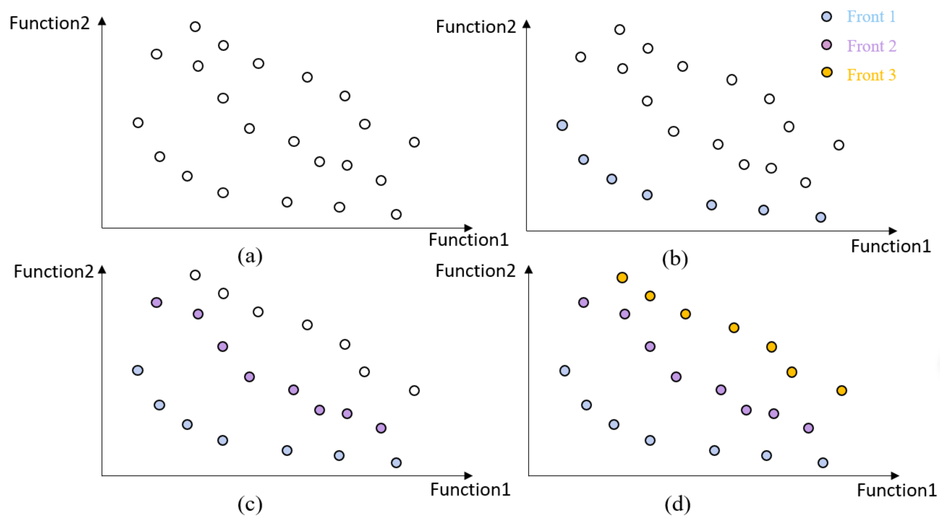
2.2.2. Pareto Optimization
- Determine the inputs and the performance of the system’s outputs (objective functions).
- Produce all the candidate retrofit solutions and determine the objective function values for all the solutions, as presented in Figure 4a.
- Determine the first front (F1) of non-dominated candidate retrofit solutions that other solutions do not dominate by using the approach, as shown in Figure 4b.
- Exclude the candidate retrofit solutions of the first front and repeat Step (3) to obtain the second Pareto optimal solutions that are only dominated by the candidate retrofit solutions of the first front, as shown in Figure 4c.
- Repeat Step (4)’s process until all candidate retrofit solutions belong to different fronts, as presented in Figure 4d.
- Rank all the candidate retrofit solutions based on the order of fronts.
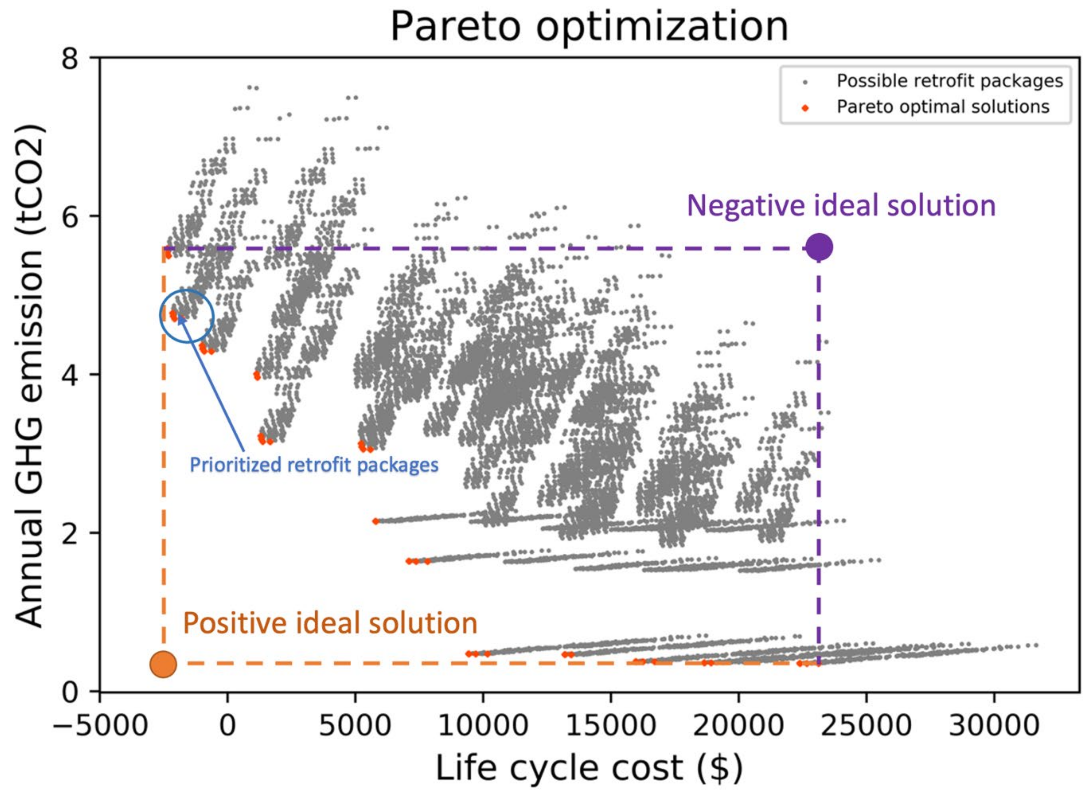
2.3. Technique for Order of Preference by Similarity to Ideal Solution
- (1)
- Weighted values of indicators
- (2)
- The positive and negative ideal solutions
- (3)
- Separation measures
- (4)
- Similarities to the positive ideal solution
3. Case Study
4. Results and Discussion
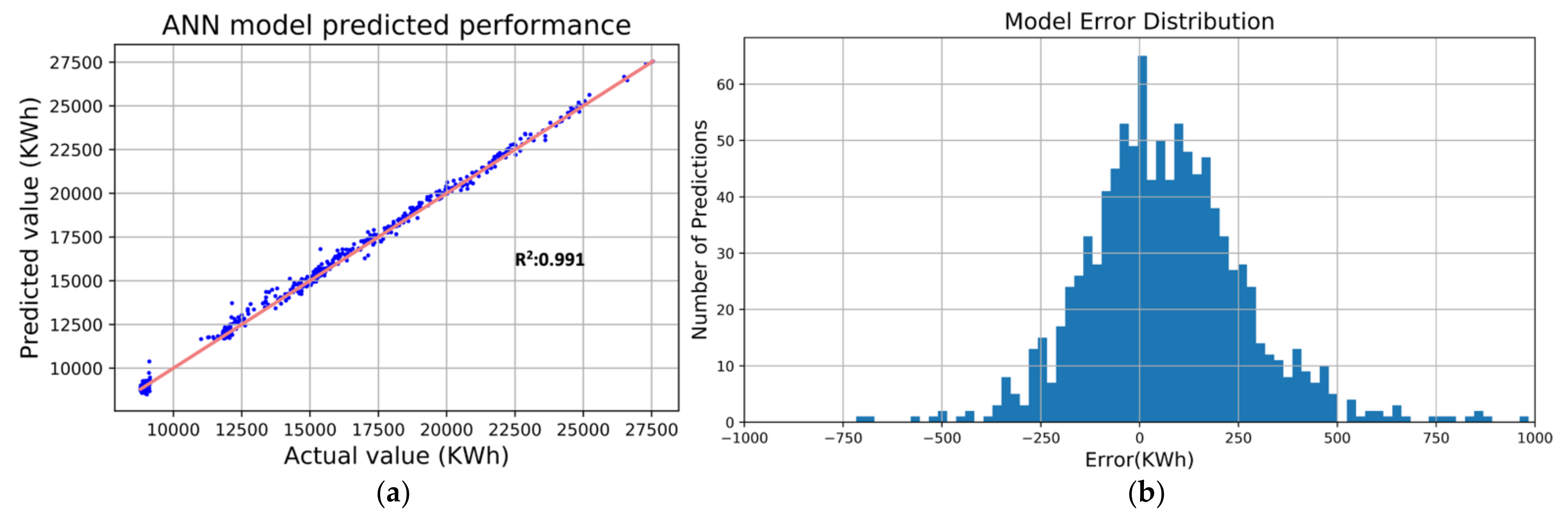
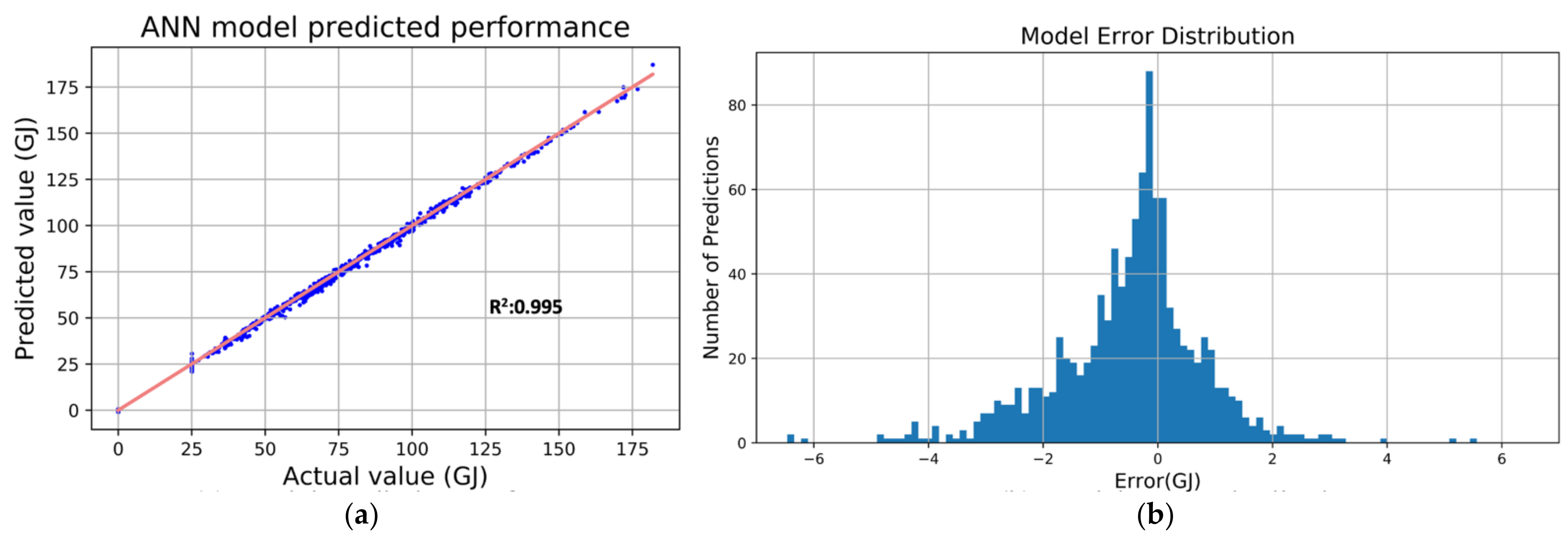
4.1. ANN Model Prediction Performance
- ANN with eight input variables and two output variables.
- Activation function: Relu function.
- Optimizer: Adam.
- Dropout rate: 0.1.
- Batch size: 64.
- Epochs: 100.
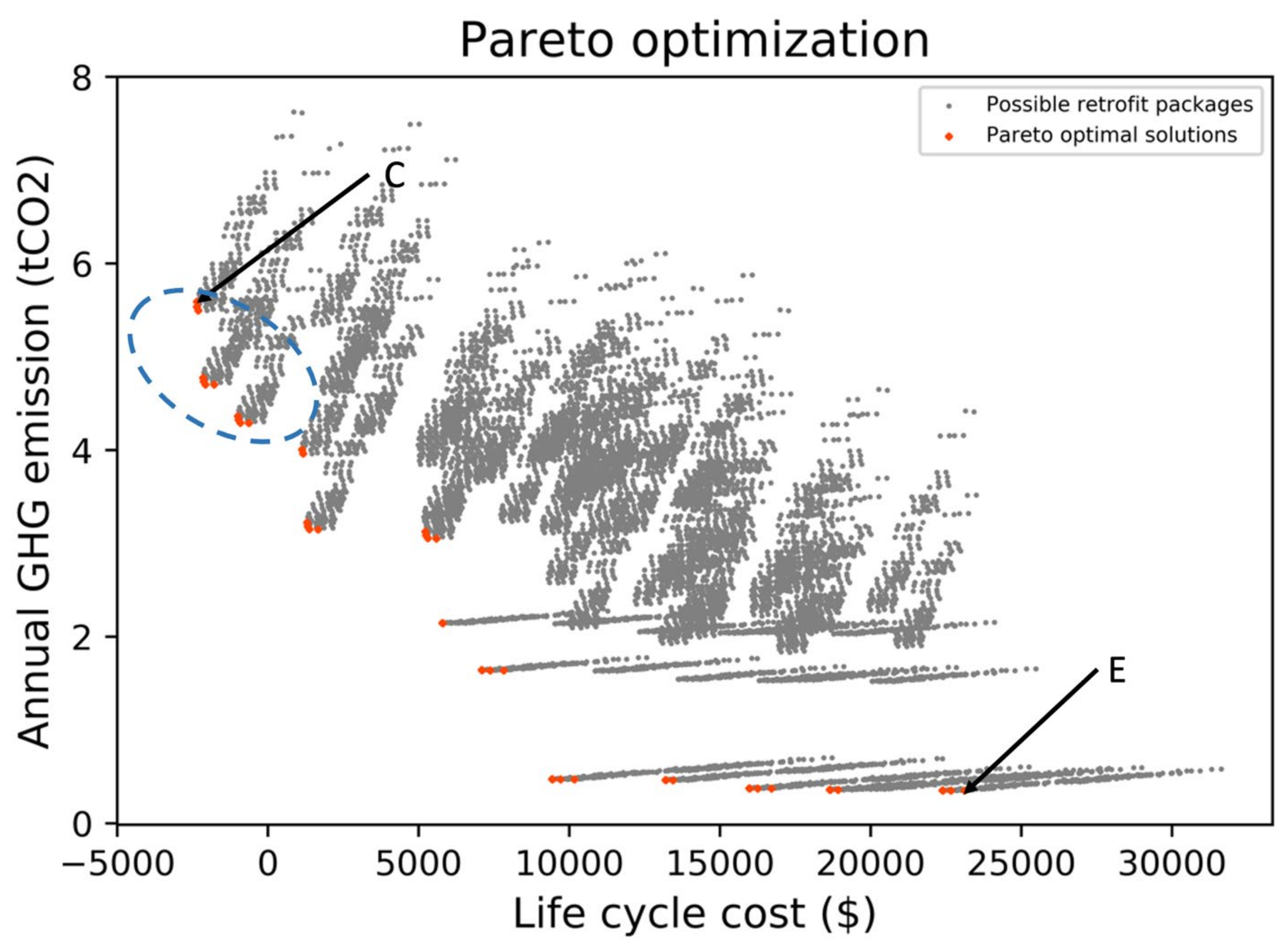
4.2. Pareto Optimal Retrofit Solutions
4.3. Prioritized Retrofit Packages
5. Conclusions
Author Contributions
Funding
Data Availability Statement
Acknowledgments
Conflicts of Interest
References
- Karunathilake, H.; Hewage, K.; Sadiq, R. Opportunities and challenges in energy demand reduction for Canadian residential sector: A review. Renew. Sustain. Energy Rev. 2018, 82, 2005–2016. [Google Scholar] [CrossRef]
- Feng, H.; Zhao, J.; Zhang, H.; Zhu, S.; Li, D. Uncertainties in whole-building life cycle assessment: A systematic review. J. Build. Eng. 2022, 50, 104191. [Google Scholar] [CrossRef]
- Natural Resources Canada. Energy and Greenhouse Gas Emissions. 2018. Available online: https://www.nrcan.gc.ca/science-data/data-analysis/energy-data-analysis/energy-facts/energy-and-greenhouse-gas-emissions-ghgs/20063 (accessed on 24 March 2022).
- Government of British Columbia. How It Works: Energy Step Code. 2018. Available online: https://energystepcode.ca/how-it-works/ (accessed on 24 March 2022).
- Prabatha, T.; Hewage, K.; Karunathilake, H.; Sadiq, R. To retrofit or not? Making energy retrofit decisions through life cycle thinking for Canadian residences. Energy Build. 2020, 226, 110393. [Google Scholar] [CrossRef]
- Zhang, H.; Hewage, K.; Prabatha, T.; Sadiq, R. Life cycle thinking-based energy retrofits evaluation framework for Canadian residences: A Pareto optimization approach. Build. Environ. 2021, 204, 108115. [Google Scholar] [CrossRef]
- Feng, H.; Liyanage, D.R.; Karunathilake, H.; Sadiq, R.; Hewage, K. BIM-based life cycle environmental performance assessment of single-family houses: Renovation and reconstruction strategies for aging building stock in British Columbia. J. Clean. Prod. 2020, 250, 119543. [Google Scholar] [CrossRef]
- Bakhtavar, E.; Prabatha, T.; Karunathilake, H.; Sadiq, R.; Hewage, K. Assessment of renewable energy-based strategies for net-zero energy communities: A planning model using multi-objective goal programming. J. Clean. Prod. 2020, 272, 122886. [Google Scholar] [CrossRef]
- Karunathilake, H.; Hewage, K.; Brinkerhoff, J.; Sadiq, R. Optimal renewable energy supply choices for net-zero ready buildings: A life cycle thinking approach under uncertainty. Energy Build. 2019, 201, 70–89. [Google Scholar] [CrossRef]
- Ma, Z.J.; Cooper, P.; Daly, D.; Ledo, L. Existing building retrofits: Methodology and state-of-the-art. Energy Build. 2012, 55, 889–902. [Google Scholar] [CrossRef]
- Ascione, F.; Bianco, N.; de Stasio, C.; Mauro, G.M.; Vanoli, G.P. Artificial neural networks to predict energy performance and retrofit scenarios for any member of a building category: A novel approach. Energy 2017, 118, 999–1017. [Google Scholar] [CrossRef]
- Pilechiha, P.; Mahdavinejad, M.; Rahimian, F.P.; Carnemolla, P.; Seyedzadeh, S. Multi-objective optimisation framework for designing office windows: Quality of view, daylight and energy efficiency. Appl. Energy 2020, 261, 114356. [Google Scholar] [CrossRef]
- Sharif, S.A.; Hammad, A. Simulation-Based Multi-Objective Optimization of institutional building renovation considering energy consumption, Life-Cycle Cost and Life-Cycle Assessment. J. Build. Eng. 2019, 21, 429–445. [Google Scholar] [CrossRef]
- Dell’Anna, F.; Bottero, M.; Becchio, C.; Corgnati, S.P.; Mondini, G. Designing a decision support system to evaluate the environmental and extra-economic performances of a nearly zero-energy building, Smart Sustain. Built Environ. 2020, 9, 413–442. [Google Scholar] [CrossRef]
- Broday, E.E.; da Silva, M.C.G. The role of internet of things (IoT) in the assessment and communication of indoor environmental quality (IEQ) in buildings: A review, Smart Sustain. Built Environ. 2022. [Google Scholar] [CrossRef]
- Birgonul, Z. A receptive-responsive tool for customizing occupant’s thermal comfort and maximizing energy efficiency by blending BIM data with real-time information, Smart Sustain. Built Environ. 2021, 10, 504–535. [Google Scholar] [CrossRef]
- Tronchin, L.; Manfren, M.; Tagliabue, L.C. Optimization of building energy performance by means of multi-scale analysis—Lessons learned from case studies. Sustain. Cities Soc. 2016, 27, 296–306. [Google Scholar] [CrossRef]
- Ascione, F.; Bianco, N.; de Stasio, C.; Mauro, G.M.; Vanoli, G.P. A new methodology for cost-optimal analysis by means of the multi-objective optimization of building energy performance. Energy Build. 2015, 88, 78–90. [Google Scholar] [CrossRef]
- Thrampoulidis, E.; Mavromatidis, G.; Lucchi, A.; Orehounig, K. A machine learning-based surrogate model to approximate optimal building retrofit solutions. Appl. Energy 2021, 281, 116024. [Google Scholar] [CrossRef]
- Hong, T.; Wang, Z.; Luo, X.; Zhang, W. State-of-the-art on research and applications of machine learning in the building life cycle. Energy Build. 2020, 212, 109831. [Google Scholar] [CrossRef] [Green Version]
- Cecconi, F.R.; Moretti, N.; Tagliabue, L.C. Application of artificial neutral network and geographic information system to evaluate retrofit potential in public school buildings, Renew. Sustain. Energy Rev. 2019, 110, 266–277. [Google Scholar] [CrossRef] [Green Version]
- Grillone, B.; Danov, S.; Sumper, A.; Cipriano, J.; Mor, G. A review of deterministic and data-driven methods to quantify energy efficiency savings and to predict retrofitting scenarios in buildings. Renew. Sustain. Energy Rev. 2020, 131, 110027. [Google Scholar] [CrossRef]
- Seyedzadeh, S.; Rahimian, F.P.; Oliver, S.; Rodriguez, S.; Glesk, I. Machine learning modelling for predicting non-domestic buildings energy performance: A model to support deep energy retrofit decision-making. Appl. Energy 2020, 279, 115908. [Google Scholar] [CrossRef]
- Miller, C.; Nagy, Z.; Schlueter, A. A review of unsupervised statistical learning and visual analytics techniques applied to performance analysis of non-residential buildings. Renew. Sustain. Energy Rev. 2018, 81, 1365–1377. [Google Scholar] [CrossRef]
- Maddalena, E.T.; Lian, Y.; Jones, C.N. Data-driven methods for building control—A review and promising future directions. Control Eng. Pract. 2020, 95, 104211. [Google Scholar] [CrossRef]
- D’Amico, A.; Ciulla, G.; Traverso, M.; Brano, V.L.; Palumbo, E. Artificial Neural Networks to assess energy and environmental performance of buildings: An Italian case study. J. Clean. Prod. 2019, 239, 117993. [Google Scholar] [CrossRef]
- Beccali, M.; Ciulla, G.; Brano, V.L.; Galatioto, A.; Bonomolo, M. Artificial neural network decision support tool for assessment of the energy performance and the refurbishment actions for the non-residential building stock in Southern Italy. Energy 2017, 137, 1201–1218. [Google Scholar] [CrossRef]
- Seyedzadeh, S.; Rahimian, F.P.; Oliver, S.; Glesk, I.; Kumar, B. Data driven model improved by multi-objective optimisation for prediction of building energy loads. Autom. Constr. 2020, 116, 103188. [Google Scholar] [CrossRef]
- Seyedzadeh, S.; Rahimian, F.P.; Rastogi, P.; Glesk, I. Tuning machine learning models for prediction of building energy loads. Sustain. Cities Soc. 2019, 47, 101484. [Google Scholar] [CrossRef]
- Martins, L.A.; Soebarto, V.; Williamson, T.; Pisaniello, D. Personal thermal comfort models: A deep learning approach for predicting older people’s thermal preference. Smart Sustain. Built Environ. 2022. [Google Scholar] [CrossRef]
- Francis, A.; Thomas, A. System dynamics modelling coupled with multi-criteria decision-making (MCDM) for sustainability-related policy analysis and decision-making in the built environment. Smart Sustain. Built Environ. 2022. [Google Scholar] [CrossRef]
- Kerdan, I.G.; Gálvez, D.M. Artificial neural network structure optimisation for accurately prediction of exergy, comfort and life cycle cost performance of a low energy building. Appl. Energy 2020, 280, 115862. [Google Scholar] [CrossRef]
- Hüthwohl, P.; Lu, R.; Brilakis, I. Multi-classifier for reinforced concrete bridge defects. Autom. Constr. 2019, 105, 102824. [Google Scholar] [CrossRef]
- Kaab, A.; Sharifi, M.; Mobli, H.; Nabavi-Pelesaraei, A.; Chau, K.W. Combined life cycle assessment and artificial intelligence for prediction of output energy and environmental impacts of sugarcane production. Sci. Total Environ. 2019, 664, 1005–1019. [Google Scholar] [CrossRef] [PubMed]
- Ouache, R.; Nahiduzzaman, K.M.; Hewage, K.; Sadiq, R. Performance Investigation of Fire Protection and Intervention Strategies: Artificial Neural Network-based Assessment Framework. J. Build. Eng. 2021, 42, 102439. [Google Scholar] [CrossRef]
- Schmidhuber, J. Deep Learning in Neural Networks: An Overview. Neural Netw. 2015, 61, 85–117. [Google Scholar] [CrossRef] [Green Version]
- Ciresan, D.; Meier, U.; Schmidhuber, J. Multi-column Deep Neural Networks for Image Classification. In Proceedings of the 2012 IEEE Conference on Computer Vision and Pattern Recognition, Providence, RI, USA, 16–21 June 2012; pp. 3642–3649. [Google Scholar] [CrossRef] [Green Version]
- Le, Q.V. Building high-level features using large scale unsupervised learning. In Proceedings of the 2013 IEEE International Conference on Acoustics, Speech and Signal Processing, Vancouver, BC, Canada, 26–31 May 2013; pp. 8595–8598. [Google Scholar] [CrossRef] [Green Version]
- Zhang, H.; Hewage, K.; Karunathilake, H.; Feng, H.; Sadiq, R. Research on policy strategies for implementing energy retrofits in the residential buildings. J. Build. Eng. 2021, 43, 103161. [Google Scholar] [CrossRef]
- ISO 15686-5:2017(en); Buildings and Constructed Assets—Service Life Planning—Part 5: Life-Cycle Costing. International Organization for Standardization: Geneva, Switzerland, 2017.
- Delmastro, C.; Mutani, G.; Corgnati, S.P. A supporting method for selecting cost-optimal energy retrofit policies for residential buildings at the urban scale. Energy Policy 2016, 99, 42–56. [Google Scholar] [CrossRef]
- Shaikh, P.H.; Shaikh, F.; Sahito, A.A.; Uqaili, M.A.; Umrani, Z. An Overview of the Challenges for Cost-Effective and Energy-Efficient Retrofits of the Existing Building Stock. In Cost-Effective Energy Efficient Building Retrofitting:Materials, Technologies, Optimization and Case Studies; Elsevier: Amsterdam, The Netherlands, 2017. [Google Scholar] [CrossRef]
- Zavadskas, E.K.; Zakarevicius, A.; Antucheviciene, J. Evaluation of Ranking Accuracy in Multi-Criteria Decisions. Informatica 2006, 17, 601–618. [Google Scholar] [CrossRef]
- MyronZhang13/MachineLearning_Python: This Is a Repository Used for the Machine Learning with Python Course. Available online: https://github.com/MyronZhang13/MachineLearning_Python (accessed on 19 April 2022).
- Galvin, R.; Sunikka-Blank, M. Economic viability in thermal retrofit policies: Learning from ten years of experience in Germany. Energy Policy 2013, 54, 343–351. [Google Scholar] [CrossRef]
- Rana, A.; Sadiq, R.; Alam, M.S.; Karunathilake, H.; Hewage, K. Evaluation of financial incentives for green buildings in Canadian landscape. Renew. Sustain. Energy Rev. 2021, 135, 110199. [Google Scholar] [CrossRef]


| ANN Hyperparameters | GA Parameters |
|---|---|
| Number of layers: 2, 3, 4 | Number of generations: 20 |
| Number of neurons per layer: 1 to 20 | Population size: 30 |
| Activation functions: Relu, Sigmoid, Elu, and Tanh | Crossover rate: 20% |
| Optimizers: Adam, SGD, Adagrad, and RMSProp | Mutation percentage: 30% |
| Dropout rate: 0, 0.1, 0.2, 0.3, 0.4 | |
| Epochs: 30, 50, 100, 200 | |
| Batch size: 32, 64, 128, 256, 512 |
| Components | Building Characteristics | Considered Retrofit Options |
|---|---|---|
| Space heating equipment | Natural gas forced air furnace with 65% annual fuel utilization efficiency (AFUE) | Natural gas furnace (92%AFUE), electric baseboard and heat pump |
| Water heating equipment | Natural gas conventional tank | Natural gas instantaneous, conventional electric tank, electric heat pump |
| Airtightness | 12 Air Change per Hour (ACH) 50 Pa | 5 ACH 50 Pa, 3.5 ACH 50 Pa |
| Above-grade wall insulation | Thermal resistance value R8.49 | Thermal resistance value R17.5, R22, R28, R30, R38 blown-in fibreglass insulation |
| Below-grade wall insulation | Thermal resistance value R3.24 | Thermal resistance value R17.5 blown-in fibreglass insulation |
| Ceiling insulation | Thermal resistance value R8.47 | Thermal resistance value R40, R50, R60 batt insulation |
| Windows | Single-glazed wood frame | Double-pane frame, triple-pane frame |
| Exterior door | Solid wood | Fibreglass polystyrene core |
| Energy Performance | RMSE | MAE | R2 |
|---|---|---|---|
| NG consumptions (GJ) | 1.384 | 0.981 | 0.995 |
| Electricity consumptions (KWh) | 226.023 | 163.552 | 0.991 |
| Rank | Prioritized Retrofit Packages | Cost Savings (Percentages) | Emission Reductions (tCO2) |
|---|---|---|---|
| 1 | Airtightness: 3.5 ACH, below-grade wall insulation: R17.5, water heating equipment: electric heat pump | 2.3 K (75%) | 1.76 |
| 2 | Airtightness: 3.5 ACH, above-grade wall insulation: R28, below-grade wall insulation: R17.5, ceiling insulation: R60, space heating equipment: natural gas furnace | 2.3 K (73%) | 1.80 |
| 3 | Above-grade wall insulation: R22, ceiling insulation: R60, water heating equipment: electric heat pump | 2.3 K (70%) | 1.84 |
| 4 | Above-grade wall insulation: R38, ceiling insulation: R40, water heating equipment: electric heat pump | 2.1 K (48%) | 2.58 |
| 5 | Airtightness: 3.5 ACH, above-grade wall insulation: R22, below-grade wall insulation: R17.5, ceiling insulation: R40, water heating equipment: natural gas, instantaneous | 2.1 K (47%) | 2.62 |
Publisher’s Note: MDPI stays neutral with regard to jurisdictional claims in published maps and institutional affiliations. |
© 2022 by the authors. Licensee MDPI, Basel, Switzerland. This article is an open access article distributed under the terms and conditions of the Creative Commons Attribution (CC BY) license (https://creativecommons.org/licenses/by/4.0/).
Share and Cite
Zhang, H.; Feng, H.; Hewage, K.; Arashpour, M. Artificial Neural Network for Predicting Building Energy Performance: A Surrogate Energy Retrofits Decision Support Framework. Buildings 2022, 12, 829. https://doi.org/10.3390/buildings12060829
Zhang H, Feng H, Hewage K, Arashpour M. Artificial Neural Network for Predicting Building Energy Performance: A Surrogate Energy Retrofits Decision Support Framework. Buildings. 2022; 12(6):829. https://doi.org/10.3390/buildings12060829
Chicago/Turabian StyleZhang, Haonan, Haibo Feng, Kasun Hewage, and Mehrdad Arashpour. 2022. "Artificial Neural Network for Predicting Building Energy Performance: A Surrogate Energy Retrofits Decision Support Framework" Buildings 12, no. 6: 829. https://doi.org/10.3390/buildings12060829
APA StyleZhang, H., Feng, H., Hewage, K., & Arashpour, M. (2022). Artificial Neural Network for Predicting Building Energy Performance: A Surrogate Energy Retrofits Decision Support Framework. Buildings, 12(6), 829. https://doi.org/10.3390/buildings12060829