A Comparative Study of Explicit and Stable Time Integration Schemes for Heat Conduction in an Insulated Wall

Abstract

Calculating heat transfer in building components is an important and nontrivial task. Thus, in this work, we extensively examined 13 numerical methods to solve the linear heat conduction equation in building walls. Eight of the used methods are recently invented explicit algorithms which are unconditionally stable. First, we performed verification tests in a 2D case by comparing them to analytical solutions, using equidistant and non-equidistant grids. Then we tested them on real-life applications in the case of one-layer (brick) and two-layer (brick and insulator) walls to determine how the errors depend on the real properties of the materials, the mesh type, and the time step size. We applied space-dependent boundary conditions on the brick side and time-dependent boundary conditions on the insulation side. The results show that the best algorithm is usually the original odd-even hopscotch method for uniform cases and the leapfrog-hopscotch algorithm for non-uniform cases.

1. Introduction

Energy efficiency in the built environment can make great contributions to a sustainable economy. Building sectors can potentially make significant reductions in energy consumption and thus in greenhouse gas emissions compared with other sectors. Heat transfer calculations in buildings are often performed for different applications such as heat loss and heat gain through the exterior envelope (heat conduction), interior environmental analyses, and material or building element-related problems [1].

Conduction heat transfer problems relevant to buildings include exterior wall conduction, interior mass conduction, conversion from heat gain/loss to cooling and heating load, and ground heat loss from the slab-on-grade floor and basement walls. The wall conduction transient heat transfer responds to climatic effects, such as temperature fluctuation, solar radiation, air convection, and so on. One of the most effective ways to improve the building energy efficiency and consumption is to improve the thermal insulation of the building envelope and reduce the heat loss through walls [2].

Heat conduction through solid materials is described by a partial differential equation (PDE), the so-called heat conduction equation or simply heat-equation, which is analogous to the diffusion equation. Analytical solutions, even new ones [3], exist for spatially homogeneous systems and most numerical methods are developed and tested by mathematicians also for these simple systems. Moreover, some analytical solutions are available for one-dimensional multilayer problems as well, for both steady-state and transient conditions. These solutions are frequently used for heat gain and loss calculations for exterior envelopes and heat storage in interior structures [1]. However, most of the building heat conduction problems are multi-dimensional and transient, while the material properties such as the density and heat conductivity can widely vary in the system [4] (p. 15). Thus, numerical computer simulation cannot be avoided.

There are lots of numerical methods to solve the heat conduction equation, such as several finite difference schemes (FDM) [5,6,7], finite element methods (FEM) [8], or a combination of these [9]. However, they can be computationally demanding since they require the full spatial discretization of the examined system. If the eigenvalues of the problem have a range of several orders of magnitude due to differences in material properties, then the problem is rather stiff and the so-called Courant–Friedrichs–Lewy (CFL) limit can be very small. This means that almost all explicit finite difference methods are unstable when the time step size is larger than this small threshold. This problem will also be demonstrated in the current paper. On the other hand, implicit methods work with the whole system matrix, thus they can be extremely slow with huge memory usage when the number of cells is large. Still, these methods are typically used for solving these kinds of equations, see for example [10,11,12,13,14,15,16].

One can observe that the trend toward increasing parallelism in high-performance computing is reinforced, since unfortunately the CPU clock frequencies nowadays increase much slower than a few decades ago [17,18]. That is one of the reasons why we believe that the importance of easily parallelizable explicit and unconditionally stable methods is going to increase, even if currently not too many scholars work with them (see [19,20,21,22,23,24,25,26] for examples).

During the last few years, our research group developed several explicit unconditionally stable methods to calculate heat conduction in arbitrary space dimensions [27,28,29,30,31,32,33,34,35,36]. Unconditional stability here means that the temperature remains finite (i.e., errors are not amplified without bounds) for arbitrary time step size. These new methods either belong to the family of FDMs or are similar to them. In those of our original papers, we tested the algorithms under general circumstances using discontinuous random parameters and initial conditions, and we have shown that they can provide quite accurate results, and they are much faster than the professionally optimized MATLAB ‘ode’ routines. In this paper, we perform systematic tests in the building walls by varying some parameters of the system and the mesh to examine how the performance of the individual methods changes and which of them is the best choice under different circumstances. We note that no comparative study has been conducted until now even about the four known explicit and stable methods examined in this paper, namely the UPFD, odd-even hopscotch, Dufort-Frankel, and rational Runge-Kutta methods (for the definitions, see the next section).

The outline of the paper is as follows: in Section 2, we present the studied system with the equations, then briefly restate the algorithms, first for the simplest case (one dimensional, equidistant mesh), then for a general, arbitrary mesh as well. In Section 3, the results of the numerical tests are presented. First, in Section 3.1, we verify our code in a 2D case by comparing the results to analytical solutions using one equidistant and some non-equidistant grids. In Section 3.2, we include the insulator, while in Section 3.3 we apply more sophisticated boundary conditions. Finally, in Section 4, we summarize our conclusions, e.g., the advantages and the disadvantages of the applied methods, and then disclose our future research plans.

2. The Studied Problem and the Methods

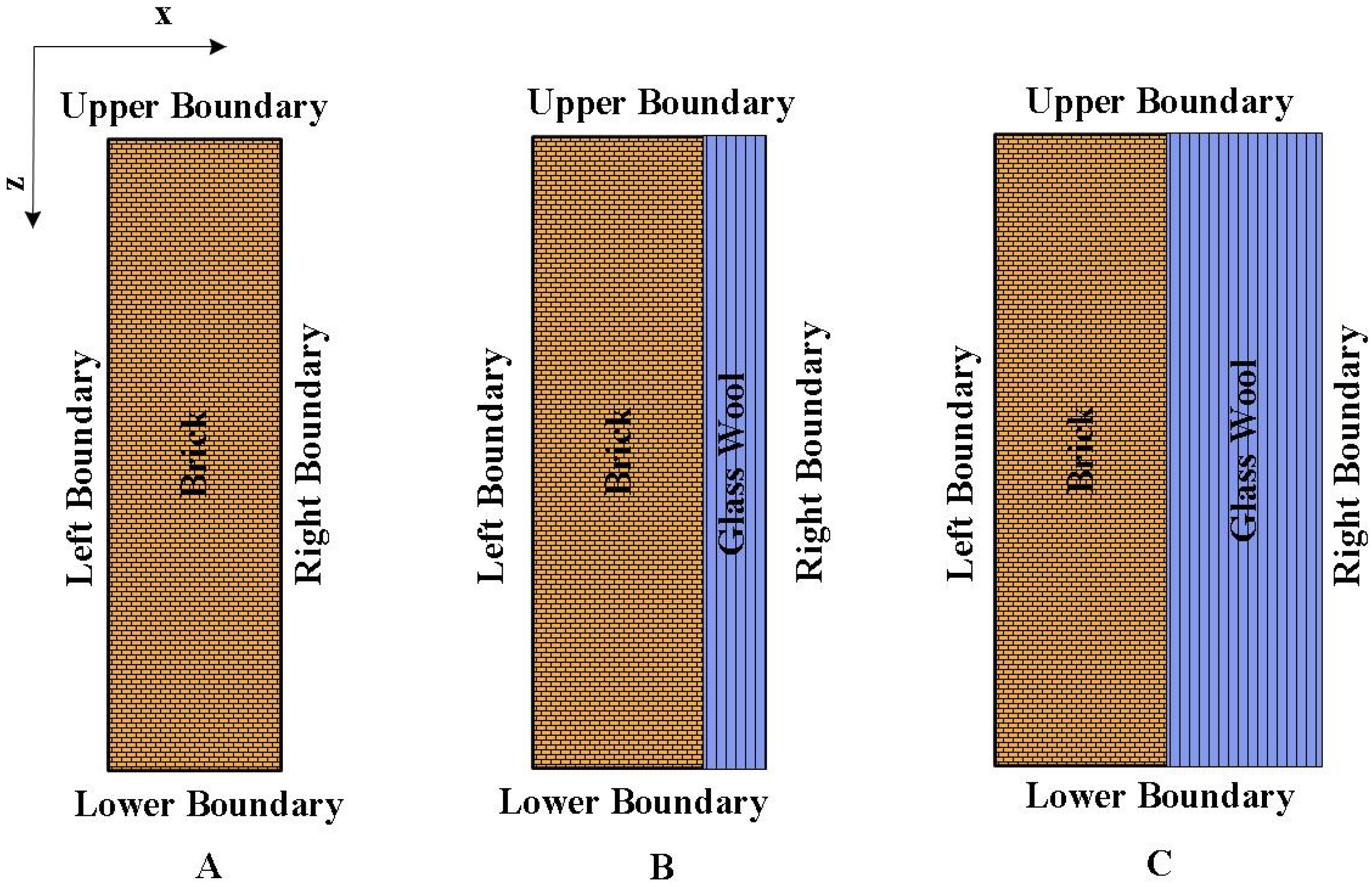
2.1. The Equation and Its Discretization and the Materials

The simplest form of the heat equation which describes the phenomenon of conduction of heat in the case of homogeneous media (typically considered by mathematicians) is the linear parabolic PDE:

$$\frac{\partial u}{\partial t}=\alpha {\nabla }^{2}u.$$

(1)

In more realistic circumstances, we can use a more general form:

$$c\rho \frac{\partial u}{\partial t}=\nabla \left(k\nabla u\right),$$

(2)

where $k=k\left(\overrightarrow{r},t\right)$, $c=c\left(\overrightarrow{r},t\right)$ and $\rho =\rho \left(\overrightarrow{r},t\right)$ are the heat conductivity, specific heat, and mass density, respectively, while $\alpha =k/(c\rho )$ is the thermal diffusivity. In the present work, we take real material properties as listed in

Table 1. The properties of the materials used.

	$\mathit{\rho } \left(\mathbf{kg}\cdot {\mathbf{m}}^{-3}\right)$	$\mathit{k}\left(\mathbf{W}\cdot {\mathbf{m}}^{-1}\cdot {\mathbf{K}}^{-1}\right)$	$\mathit{c}\left(\mathbf{J}\cdot {\mathbf{kg}}^{-1}\cdot {\mathbf{K}}^{-1}\right)$
Brick	1600	0.73	800
Glass wool	200	0.03	800

.

As one can see in Figure 1, we considered a one-layer wall consisting of brick only and two-layer walls consisting of brick and glass wool insulator.

In case of Equation (1) in one dimension, we apply the most standard central difference formula

$$\frac{{\partial }^2}{\partial x^2}u(x_i)\approx \frac{\frac{u(x_{i+1})-u(x_i)}{\Delta x}+\frac{u(x_{i-1})-u(x_i)}{\Delta x}}{\Delta x}=\frac{u_{i-1}-2u_i+u_{i+1}}{\Delta x^2},$$

which is second order in $\Delta x$. Let us now present the discretization of Equation (2) based on the usual discretization of Equation (1). One can find more details about this procedure in Chapter 5 of book [37] for the case of underground reservoirs. Let us suppose that α, k, c, and ρ, the quantities describing the properties of materials, are functions of the space (and time) variables instead of being constants. Examine a one-dimensional, equidistant grid and discretize the second-order space derivatives by the standard central difference formula, where k is a function of x and cannot be simply merged with c and ρ. Thus, we have

$${c(x_i)\rho (x_i)\frac{\partial u}{\partial t}|}_{x_i}=\frac{1}{\Delta x}\left[k\left(x_i+\frac{\Delta x}{2}\right)\frac{u(x_i+\Delta x)-u(x_i)}{\Delta x}+k\left(x_i-\frac{\Delta x}{2}\right)\frac{u(x_i-\Delta x)-u(x_i)}{\Delta x}\right].$$

We change now from node to cell variables, thus $u_i$, ${\rho }_i$, and $c_i$ will be the (average) temperature, density, and specific heat of cell i, respectively, while $k_{i,i+1}$ will be the heat conductivity between cell i and its (right) neighbor. The previous equation will have the form

$$\frac{d{u}_i}{dt}=\frac{1}{c_i{\rho }_i\Delta x}\left(k_{i,i+1}\frac{u_{i+1}-u_i}{\Delta x}+k_{i-1,i}\frac{u_{i-1}-u_i}{\Delta x}\right).$$

We turn to a non-equidistant grid with non-uniform cross section, which is still one-dimensional. If the length and the (average) cross section of the cell is denoted by $\Delta x_i$ and $A_i$, we can write the distance between the center of the cell i and its neighbor j as $d_{ij}=\left(\Delta x_i+\Delta x_j\right)/2$. The area of the interface between the two neighboring cells can be approximated as $A_{i,i\pm 1}\approx A_i\approx A_{i\pm 1}$. Now one can write, more generally than in the previous equation, that

$$\frac{d{u}_i}{dt}=\frac{1}{c_i{\rho }_i\Delta x_i{A}_i}\left(A_{i,i+1}{k}_{i,i+1}\frac{u_{i+1}-u_i}{d_{i,i+1}}+A_{i,i-1}{k}_{i,i-1}\frac{u_{i-1}-u_i}{d_{i,i-1}}\right).$$

The volume and the heat capacity of the cell can be calculated as $V_i=A_i\Delta x_i$ and $C_i=c_i{\rho }_i{V}_i$, respectively, while the thermal resistance between these neighboring cells can be estimated as $R_{ij}\approx d_{ij}/k_{ij}{A}_{ij}$. If one uses these new quantities, the following expression for the time derivative of each cell-variable is obtained:

$$\frac{d{u}_i}{dt}=\frac{u_{i-1}-u_i}{R_i{{}_{-1,}}_i{C}_i}+\frac{u_{i+1}-u_i}{R_i{{}_{+1,}}_i{C}_i}.$$

This can be straightforwardly generalized further, thus the spatially discretized form of Equation (2) with an arbitrary number of neighbors can be written as follows:

$$\frac{d{u}_i}{dt}={\displaystyle \sum _{j\ne i}\frac{u_j-u_i}{R_{i,j}{C}_i}}.$$

(3)

This system of an ordinary differential equation can be used in the case of arbitrary (e.g., unstructured) grids consisting of cells of various shapes and properties. Of course, this kind of discretization can modify the spatial accuracy, but we will see during the verification that the error due to this space discretization is still small.

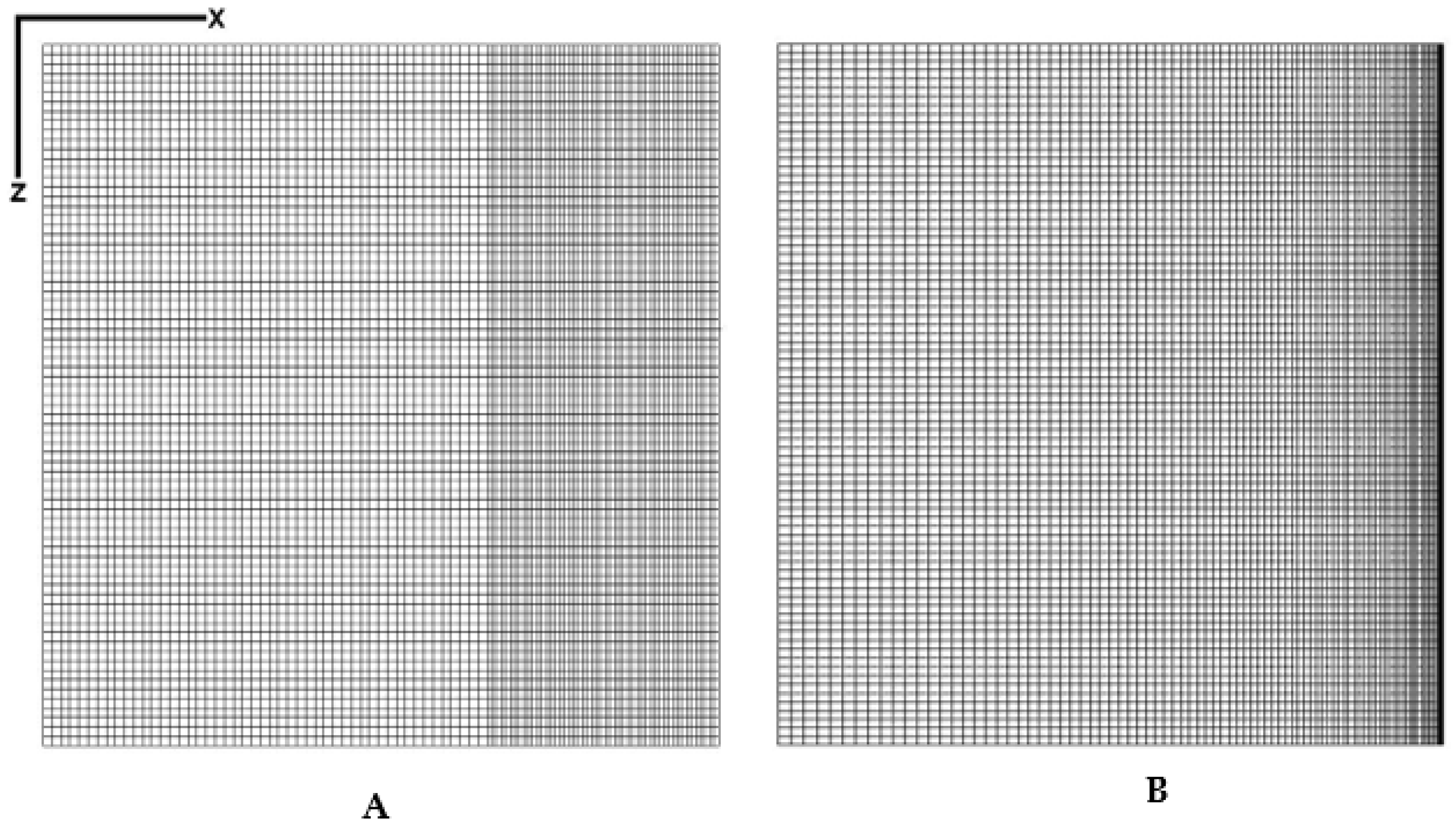
2.2. Mesh Construction

We considered a piece of wall with volume 1 m $\times$ 1 m $\times$ 1 m. However, no physical quantities are changing in the y-direction (perpendicular to the surface of Figure 1 and Figure 2), thus that dimension is irrelevant. It means we deal only with a cross-section, which is a two-dimensional problem from the mathematical point of view and thus we can use $\Delta y_i=1$. So, we constructed several meshes of size 1 m², which means $\left(x,z\right)\in \left[0, 1\right]\times \left[0, 1\right]$. The shape of the cells is square in the equidistant mesh and rectangular in the non-equidistant meshes. The heat capacity of the cells can be given as $C_i=c_i{\rho }_i\Delta x_i\Delta z_i$, while the thermal resistance in the x-direction has the approximate formula $R{x}_i\approx \frac{\Delta x_i}{k_{i}A{x}_i}$, where $A{x}_i$ is the surface element perpendicular to x. Since now it can be given as $A{x}_i=\Delta y_i\Delta z_i=\Delta z_i$, the horizontal and vertical resistances can be given in case of a homogeneous material and uniform mesh as

$$R{x}_i\approx \frac{\Delta x_i}{k_i\Delta z_i} \mathrm{and} R{z}_i\approx \frac{\Delta z_i}{k_i\Delta x_i},$$

respectively. If the material properties or the sizes of the two neighboring cells are different, we can write for the resistance between cells i and i + 1 that

$$R{x}_i\approx \frac{\Delta x_i}{2k_i\Delta z_i}+\frac{\Delta x_{i+1}}{2k_{i+1}\Delta z_{i+1}},$$

and if the cell j is below the cell i, we have

$$R{z}_i\approx \frac{\Delta x_i}{2k_i\Delta z_i}+\frac{\Delta x_j}{2k_j\Delta z_j}$$

for the vertical resistance.

We apply an equidistant grid and some non-equidistant grids to discretize the space variables in both the one layer and the multilayer cases. The cell number along axis x is set to N_x = 100. Similarly, the cell number along axis z is N_z = 100, except in Section 3.3 where $N_x=N_z=80$. Thus, we have a grid with a total cell number $N=N_x{N}_z = \mathrm{10,000}$ (and $N=6400$ in Section 3.3). We have to note that the temperature in the middle of the cell was considered the temperature of the cell. However, we are going to use Dirichlet boundary conditions to reproduce an analytical solution, therefore the boundary of the system should be in the middle of the cells belonging to the boundary. This issue is solved by increasing the size of the cells, so in the case of an equidistant grid and $N_x=N_z=100$, we have $\Delta x=\Delta z=0.0101$ instead of just 0.01.

We also wanted to consider wide cells on the left side of the wall and small ones on the right side of the wall. We implemented this in two different ways. In case of abrupt change, we used an equidistant coarse mesh $\Delta x=0.0105$ at the left 50% of the cells, and an equidistant fine mesh $\Delta x=0.0097$ at the right side.

For a gradual change, the width of the cells were decreased as a geometric series as follows. For $r\ne 1$, the sum of the first n + 1 terms of a geometric series, up to and including the rⁿ term, is

$$a+ar+a{r}^2+a{r}^3+\dots \dots +a{r}^n={\displaystyle \sum _{k=0}^{n}a{r}^k=a\left(\frac{1-r^{n+1}}{1-r}\right)}$$

We used r = 0.98, $n=N_x-1$, and a = 0.0234. This means that on the left side $\Delta x_1=0.0234$ and it is gradually decreased to $\Delta x_{N_x}={0.98}^{99}\cdot \Delta x_1=0.00317$. The same abrupt and gradual change can be implemented in the z-direction.

In the multilayer case, the left 50% of the cells were always brick and the right 50% were insulator. It implies that, if the mesh is equidistant, the volume of the brick and the insulator is the same as in Figure 1C. However, if we have abrupt or gradual change in the x-direction, the thickness of the insulator is smaller, similar to the case in Figure 1B.

We always use equidistant temporal discretization with time step size $\Delta t$, and $u_i^n$ denotes the temperature of cell i at time moment $n\Delta t$.

2.3. The Initial and the Boundary Conditions

We applied different initial and boundary conditions for both the one layer and the multilayer cases as follows:

• Sinusoidal initial condition with zero Dirichlet boundary condition.

The initial condition is the product of two sine functions:

$$u(x,z,t=0)=\sin (\pi x)\sin (\pi z).$$

(4)

The simplest zero Dirichlet boundary conditions are used:

$$u(x=0,z,t)=u(x=1,z,t)=u(x,z=0,t)=u(x,z=1,t)=0.$$

(5)

Anyone can easily check that the analytical solution to this problem is

$$u(x,z,t)=\sin (\pi x)\sin (\pi y){\mathrm{e}}^{-2{\pi }^{2}t},$$

(6)

valid only in homogeneous material, i.e., in a one-layer wall.

II.

Linear initial condition with combined boundary conditions.

The initial condition is a linear function of the z variable:

$$u\left(x,z, t=0\right)=30-15z.$$

Neumann boundary condition at the top and bottom of the wall, meaning thermal isolation:

$$u_z(x,z=0,t)=u_z(x,z=1,t)=0.$$

Space-dependent temperature at the left boundary:

$$u\left(x=0, z,t\right)=30-15z.$$

Time-dependent temperature at the right boundary:

$$u\left(x=1, z,t\right)=\mathrm{u}\left(x=1, z=0,t=0\right)\cdot {\mathrm{e}}^{\lambda \mathrm{t}},$$

where $\lambda$ = 0.00004. Since the final time was 10,000, it means that the temperature at the right boundary is gradually increased from $30 °\mathrm{C}$ to $44.75 °\mathrm{C}$.

We note that in case II we chose such complicated boundary conditions to demonstrate that the methods perform well even in these cases.

2.4. The Applied Numerical Methods

In this section, we give essential information about the algorithms. We first present their formula for the simplest case (one dimensional, equidistant mesh, Equation (1)), then immediately for a general, arbitrary mesh as well. The simplest form is useful for comparison purposes, since numerical schemes are given in this form in most textbooks on numerical methods. The more general forms are necessary because we use only them in this work.

We introduce the usual mesh-ratio $r=\frac{\alpha \Delta t}{\Delta x^2}$ for the 1D equidistant mesh, e.g., for Equation (1). On the other hand, for the case of the general mesh, we introduce the following notations

$$r_i=\Delta t{\displaystyle \sum _{j\ne i}\frac{1}{C_i{R}_{ij}}} \mathrm{and} A_i=\Delta t{\displaystyle \sum _{j\ne i}\frac{u_j^n}{C_i{R}_{ij}}}.$$

(7)

The first quantity is the generalization of r (defined above), while the second one reflects the state and the effect of the neighbors of cell i as well.

1.

The constant neighbor (CNe) method [28,38] for Equation (1) is:

$$u_i^{n+1}=u_i^n\cdot e^{-2r}+\frac{u_{i-1}^n+u_{i+1}^n}{2}\left(1-e^{-2r}\right)$$

While for general grids it is:

$$u_i^{n+1}=u_i^n\cdot e^{-r_i}+\frac{A_i}{r_i}\left(1-e^{-r_i}\right)$$

To proceed, let us recall that the following general time discretization

$$\frac{u_i^{n+1}-u_i^n}{\Delta t}=\frac{\alpha }{\Delta x^2}\left[\theta \left(u_{i-1}^n-2u_i^n+u_{i+1}^n\right)+\left(1-\theta \right)\left(u_{i-1}^{n+1}-2u_i^{n+1}+u_{i+1}^{n+1}\right)\right],$$

implies the so-called theta method:

$$u_i^{n+1}=u_i^n+r\left[\theta \left(u_{i-1}^n-2u_i^n+u_{i+1}^n\right)+\left(1-\theta \right)\left(u_{i-1}^{n+1}-2u_i^{n+1}+u_{i+1}^{n+1}\right)\right],$$

(8)

where $\theta \in \left[0,1\right]$. For $\theta =0,\raisebox{1ex}{$1$}\!\left/ \!\raisebox{-1ex}{$2$}\right., \mathrm{and} 1$ one has the (standard) implicit Euler, the Crank–Nicolson, and the explicit Euler (FTCS) schemes, respectively [39]. If $\theta <1$, the theta method is implicit. It can be modified to be explicit by taking the neighbors into account at the old time level, where their values are already calculated. Thus, one can insert $u_{i\pm 1}^n$ into the theta-scheme (8) instead of $u_{i\pm 1}^{n+1}$ to obtain

$$u_i^{n+1}=u_i^n-2r\theta u_i^n-2r\left(1-\theta \right)u_i^{n+1}+r\left(u_{i-1}^n+u_{i+1}^n\right).$$

With this modification, the final formula is completely explicit:

$$u_i^{n+1}=\frac{\left(1-2r\theta \right)u_i^n+r\left(u_{i-1}^{n+1}+u_{i+1}^{n+1}\right)}{1+2r\left(1-\theta \right)}.$$

(9)

2.

The UPFD method is the theta-method (9) for $\theta =0$. In the case of Equation (1), it reads as follows:

$$u_i^{n+1}=\frac{u_i^n+r\left(u_{i-1}^n+u_{i+1}^n\right)}{1+2r},$$

(10)

and the general form for Equation (2) or (3) is:

$$u_i^{n+1}=\frac{u_i^n+A_i}{1+2r_i}.$$

(11)

3.

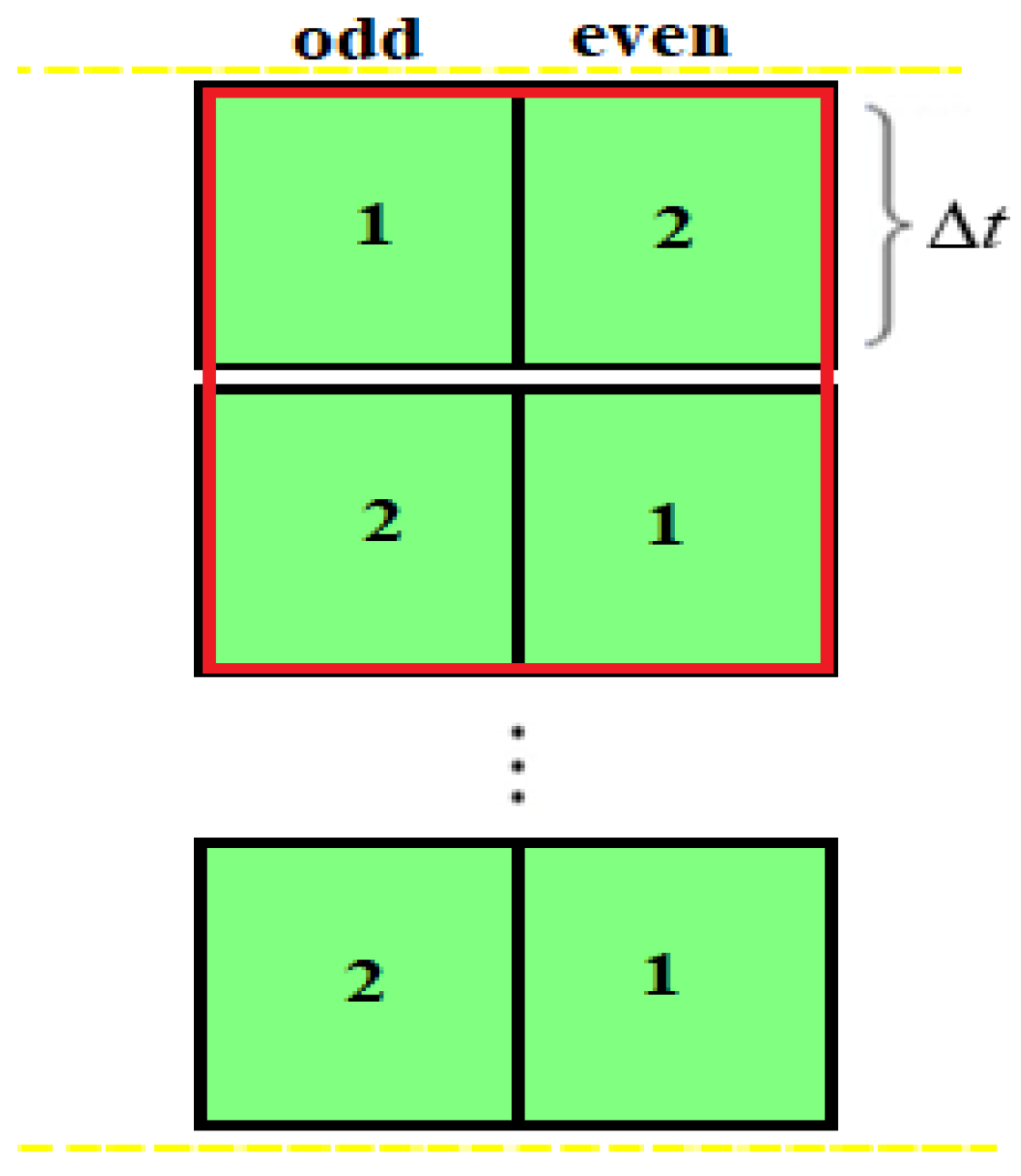
If we would like to apply an odd-even hopscotch method, we need a bipartite grid, where all the nearest neighbors of the odd cells are even and vice versa. In the original odd-even hopscotch (OOEH) method [40], the standard explicit Euler formula was applied in the first stage and the implicit Euler formula was applied in the second stage, as is shown in Figure 3. The special and the general formulas are the following:

$$\mathrm{Explicit} \mathrm{Euler}: u_i^{n+1}=\left(1-2r\right)u_i^n+r\left(u_{i-1}^n+u_{i+1}^n\right) \mathrm{and} u_i^{n+1}=\left(1-r_i\right)u_i^n+A_i.$$

$$\mathrm{Implicit} \mathrm{Euler}: u_i^{n+1}=\frac{u_i^n+r\left(u_{i-1}^{n+1}+u_{i+1}^{n+1}\right)}{1+2r} \mathrm{and} u_i^{n+1}=\frac{u_i^n+A_i^{\mathrm{new}}}{1+r_i},$$

where $A_i^{\mathrm{new}}$ is calculated in the same way as $A_i$ in (7), but using the new values of the temperatures, which make the implicit formula effectively explicit.

Figure 3. Space-time structure of the hopscotch (OOEH) method.

Figure 3. Space-time structure of the hopscotch (OOEH) method.

As we will see, this is a powerful explicit method, but in stiff cases, its error can be extremely large [32].

4.

The reversed odd-even hopscotch method (ROEH) applies the formulas of the OOEH method in the opposite order. However, since the new values of the neighbors are not known when first-stage calculations begin, the implicit formula can be applied only with a trick, which is that of the UPFD method, see Formulas (10) and (11). Obtaining the code of this method is easy, since one only needs to change the order of the two formulas in the code of the original OOEH. We showed that this method produces much smaller errors in the case of very stiff systems than the OOEH method [32].

5.

The next method is the two-stage linear-neighbor (LNe or LNe2) method [38]. It is based on the CNe method, which is used as a predictor to calculate new $u_i^{\mathrm{pred}}$ values valid at the end of the actual time step. Using them we can calculate slopes.

$$s_i=\frac{r}{\Delta t^2}\left(u_{i-1}^{\mathrm{pred}}+u_{i+1}^{\mathrm{pred}}-u_{i-1}^n-u_{i+1}^n\right)$$

and then the corrector values for the two-stage LNe method:

$$u_i^{n+1}=u_i^n{e}^{-2r}+\frac{u_{i-1}^n+u_{i+1}^n}{2}\left(1-e^{-2r}\right)+s_i\frac{\Delta t^2}{2r}\left(1-\frac{1-e^{-2r}}{2r}\right).$$

For the general case,

$$A_i^{\mathrm{new}}=\Delta t{\displaystyle \sum _{j\ne i}\frac{u_j^{\mathrm{pred}}}{C_i{R}_{\mathrm{ij}}}},$$

(12)

with which we can make the corrector step as follows:

$$u_i^{n+1}=u_i^n{e}^{-r_i}+\left(A_i-\frac{A_i^{\mathrm{new}}-A_i}{r_i}\right)\frac{1-e^{-r_i}}{r_i}+\frac{A_i^{\mathrm{new}}-A_i}{r_i}.$$

(13)

6.

The values given in Equation (13) can be used to recalculate $A_i^{\mathrm{new}}$ again, which makes sense to repeat (13) to obtain new results. In this case, we have three stages altogether, thus the method is called the LNe3 method [38]. This algorithm is still second order, but more accurate than LNe2.

7.

The CpC algorithm [35] generally starts with a fractional time step with length $p\Delta t$, but here we take $p=\raisebox{1ex}{$1$}\!\left/ \!\raisebox{-1ex}{$2$}\right.$, because this version usually has better accuracy than for other values of p. So, in the first stage, we calculate new predictor values of the variables with the CNe formula, but with a $\Delta t_1=\Delta t/2$ time step:

$$u_i^{\mathrm{pred}}=u_i^n\cdot e^{-r}+\frac{u_{i-1}^n+u_{i+1}^n}{2}\left(1-e^{-r}\right) \mathrm{and} u_i^{\mathrm{pred}}=u_i^n{e}^{-r_i/2}+\frac{A_i}{r_i}\left(1-e^{-r_i/2}\right).$$

In the second stage, we can use (12) with $\Delta t_1$ and take a full-time step size corrector step using the CNe formula again. Thus, the final values at the end of the time step are

$$u_i^{n+1}=u_i^n\cdot e^{-2r}+\frac{u_{i-1}^{\mathrm{pred}}+u_{i+1}^{\mathrm{pred}}}{2}\left(1-e^{-2r}\right) \mathrm{and} u_i^{n+1}=u_i^n\cdot e^{-r_i}+\frac{A_i^{\mathrm{new}}}{r_i}\left(1-e^{-r_i}\right)$$

8.

Heun’s method, also called explicit trapezoidal rule, may be the most common second-order RK scheme [41]. It starts with an explicit Euler stage as a predictor:

$$u_i^{\mathrm{pred}}=\left(1-2r\right)u_i^n+r\left(u_{i-1}^n+u_{i+1}^n\right) \mathrm{and} u_i^{\mathrm{pred}}=\left(1-r_i\right)u_i^n+A_i,$$

then, using the average of the obtained and the old values a corrector-step follows:

$$u_i^{n+1}=u_i^n-r\left(u_i^n+u_i^{\mathrm{pred}}\right)+r\frac{u_{i-1}^n+u_{i-1}^{\mathrm{pred}}+u_{i+1}^n+u_{i+1}^{\mathrm{pred}}}{2}$$

and

$$u_i^{n+1}=u_i^n-r_i\frac{u_i^n+u_i^{\mathrm{pred}}}{2}+\frac{A_i+A_i^{\mathrm{new}}}{2}.$$

9.

In the case of the pseudo-implicit (PI) method, we took Algorithm 5 from [36] in the case of the pure heat equation with parameter setting $\lambda =1$, which gives the following two-stage algorithm for the special case:

$$Stage 1: u_i^{\mathrm{pred}}=\frac{u_i^n+\raisebox{1ex}{$r$}\!\left/ \!\raisebox{-1ex}{$2$}\right.\left(u_{i-1}^n+u_{i+1}^n\right)}{1+r}$$

$$Stage 2: u_i^{n+1}=\frac{\left(1-r\right)u_i^n+r\left(u_{i-1}^{\mathrm{pred}}+u_{i+1}^{\mathrm{pred}}\right)}{1+r}$$

For a general grid, we have

$$Stage 1: u_i^{\mathrm{pred}}=\frac{u_i^n+A_i}{1+r_i}, \mathrm{where} A_i=\frac{\Delta t}{2}{\displaystyle \sum _{j\ne i}\frac{u_j^n}{C_i{R}_{\mathrm{ij}}}}$$

$$Stage 2: u_i^{n+1}=\frac{\left(1-r_i\right)u_i^n+A_i^{\mathrm{new}}}{1+r_i}, \mathrm{where} A_i^{\mathrm{new}}=\Delta t{\displaystyle \sum _{j\ne i}\frac{u_j^{\mathrm{pred}}}{C_i{R}_{\mathrm{ij}}}}.$$

10.

The Dufort–Frankel (DF) algorithm can be obtained from the so-called leapfrog explicit scheme by a modification [42] (p. 313). It is a known explicit unconditionally stable scheme that has the formula in the special and general case:

$$u_i^{n+1}=\frac{\left(1-2r\right)u_i^{n-1}+2r\left(u_{i-1}^n+u_{i+1}^n\right)}{1+2r} \mathrm{and} u_i^{n+1}=\frac{\left(1-r_i\right)u_i^{n-1}+2A_i}{1+r_i}.$$

As one can see, it is a one-stage but two-step method (the formula contains $u_i^{n-1}$), which is not self-starter, so another method must be applied to start the method by the calculation $u_i^1$. For this purpose, we apply the UPFD formula twice (with halved time step size).

11.

Rational Runge-Kutta methods are a family of nonlinear methods, which means that the new $u_i^{n+1}$ values are not the linear combinations of the old $u_i^n$ values. We chose a two-stage version [43] defined as follows. The first stage is a full step by the explicit Euler (FTCS) to obtain the predicted value:

$$\begin{array}{c}{g}_i^1=r\left(u_{i-1}^n-2u_i^n+u_{i+1}^n\right) \mathrm{and} g_i^1=-r{u}_i^n+A_i\\ u_i^{\mathrm{pred}}=u_i^n+g_i^1\end{array}$$

Then, the increment of a repeated Euler-step is calculated, using the predictor values obtained above:

$$g_i^2=r\left(u_{i-1}^{\mathrm{pred}}-2u_i^{\mathrm{pred}}+u_{i+1}^{\mathrm{pred}}\right) \mathrm{and} g_i^2=-r_i{u}_i^{\mathrm{pred}}+A_i^{\mathrm{new}}$$

If we introduce the scalar products, which are common for the cells, they need to be calculated only once in a time step, thus we can write

$$p_1=\left({\overrightarrow{g}}^1,{\overrightarrow{g}}^1\right)={\displaystyle \sum _{i=1}^N{g}_i^1{g}_i^1},p_{12}=\left({\overrightarrow{g}}^1,{\overrightarrow{g}}^2\right)={\displaystyle \sum _{i=1}^N{g}_i^1{g}_i^2},p_2=\left({\overrightarrow{g}}^2,{\overrightarrow{g}}^2\right)={\displaystyle \sum _{i=1}^N{g}_i^2{g}_i^2},$$

we then obtain the final expression for the new variables:

$$u_i^{n+1}=u_i^n+\frac{2p_1{g}_i^1-2p_{12}{g}_i^1+p_1{g}_i^2}{4p_1-4p_{12}+p_2}.$$

12.

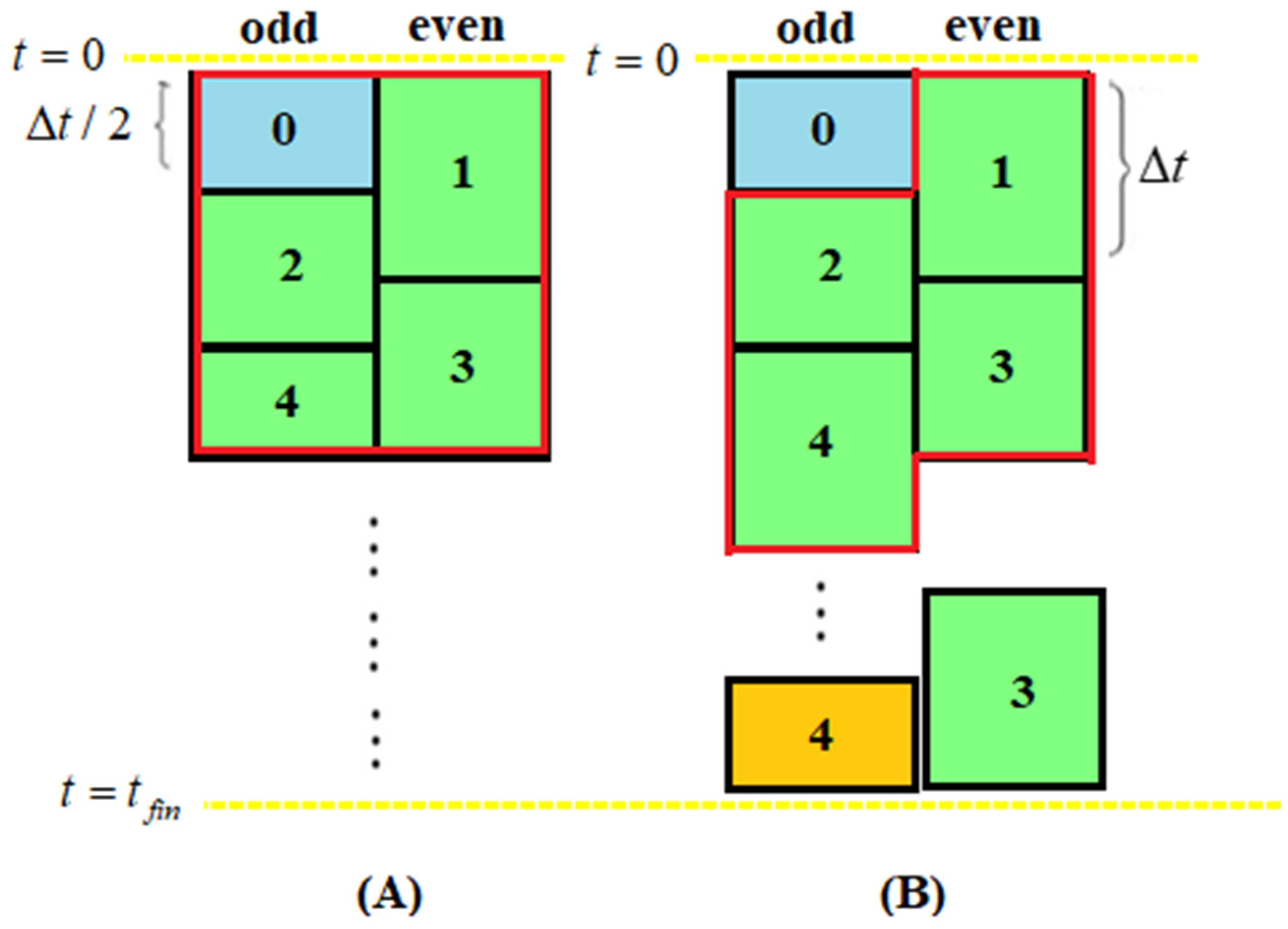
In the shifted-hopscotch (SH) method [33], we have a repeating block consisting of five stages, which corresponds to two half and three full-time steps, which altogether span two time steps for odd as well as even cells, as one can see in Figure 4A. The calculation starts with a half-sized time step for the odd cells which is symbolized by a light blue box with the number 1 in the figure. Then, a full-time step for the even, the odd, and the even cells follows again. Finally, a half-size time step for the odd cells closes the calculation of the values. In our original work [33] we used the $\theta$ Formula (9)

$$u_i^{\mu +1}=\frac{\left(1-2r\theta \right)u_i^{\mu }+r\left(u_{i-1}^{\mu +\raisebox{1ex}{$1$}\!\left/ \!\raisebox{-1ex}{$2$}\right.}+u_{i+1}^{\mu +\raisebox{1ex}{$1$}\!\left/ \!\raisebox{-1ex}{$2$}\right.}\right)}{1+2r\left(1-\theta \right)},$$

(14)

and (in the general case),

$$u_i^{\mu +1}=\frac{\left(1-r_i\theta \right)u_i^{\mu }+A_i}{1+r_i\left(1-\theta \right)}.$$

(15)

Figure 4. (A) The shifted-hopscotch structure. (B) The leapfrog-hopscotch structure.

Figure 4. (A) The shifted-hopscotch structure. (B) The leapfrog-hopscotch structure.

In this paper, we use only the combination already proven to be the best (S4 in [33]), which means $\theta =0$ is used at the first, $\theta =1$ at the fifth, and $\theta =\raisebox{1ex}{$1$}\!\left/ \!\raisebox{-1ex}{$2$}\right.$ in all other stages. The upper index containing µ means that always the latest available values are used when the new values of u are calculated, regardless of the size of the time step.

13.

Finally, in the leapfrog-hopscotch (LH) method [34] we have a structure consisting of two half and several full time steps. The calculation starts again by taking a half-sized time step for the odd nodes using the initial values, then, for the even and odd nodes, full-time steps are taken strictly alternately until the end of the last timestep (orange box in Figure 4B), which should be halved for odd nodes to reach the same final time point as the even nodes. In this paper, we used only the best already proven combination of formulas (L2 in [34]), which means that $\theta =0$ and $\theta =\raisebox{1ex}{$1$}\!\left/ \!\raisebox{-1ex}{$2$}\right.$ are applied in Formulas (14) and (15) at the first and at all other time steps, respectively.

The CNe and the UPFD methods are first order while all other methods are second order in time step size. All the methods used, except, of course, Heun’s method, are unconditionally stable for the linear heat conduction equation, i.e., the previously mentioned CFL limit is not relevant for them. This, however, does not mean they are always accurate. Actually, the price of unconditional stability is conditional consistency, which means that spatial mesh refinement with a constant time step size yields worsening accuracy (in contrast to worsening stability properties as in mainstream methods), which is examined analytically and numerically in our previous papers [44] and [35], respectively. In Section 3.2 we will show examples when the conditionally stable Heun’s method is significantly more accurate for small time step sizes than our methods. We emphasize again that very few explicit methods are unconditionally stable, e.g., no explicit Runge-Kutta method can be A-stable [45] (p. 60).

3. Results

We define the (global) error as the largest absolute difference between the reference temperature $u_i^{\mathrm{ref}}$ and the temperature $u_i^{\mathrm{num}}$ obtained by the studied numerical method at $t_{\mathrm{fin}}=\mathrm{10,000} \left(\mathrm{s}\right)$, which is the end of the examined time interval:

$$MaxError=\underset{1\le i\le N}{\max }\left|u_i^{\mathrm{ref}}(t_{\mathrm{fin}})-u_i^{\mathrm{num}}(t_{\mathrm{fin}})\right|.$$

(16)

The reference solution is either the analytical solution (6) of the PDE or a numerical solution obtained by applying Heun’s method with an extremely small time step size $\Delta t=0.002$. We have chosen Heun’s method for reference because this is the most widely tested algorithm among the examined methods.

If the grid is not uniform, it makes sense to calculate the so-called energy error:

$$\mathrm{Error}(Energy)={\displaystyle \sum _{1\le j\le N}{C}_j\left|u_j^{\mathrm{ref}}(t_{\mathrm{fin}})-u_j^{\mathrm{num}}(t_{\mathrm{fin}})\right|},$$

(17)

where C is the heat capacity defined in Section 2.1 and Section 2.2. This tells us how much energy in the system is not in the proper cell.

For a given problem, spatial mesh, and method, the error is a function of the time step size. We start with a very large time step size $\Delta t$, calculate the error and then decrease $\Delta t$ by a factor of two until reaching small error values to comprehensively investigate the behavior of the methods.

For the simulations where running times are measured, we used a desktop computer with an Intel Core i7-11700 CPU and 64 GB RAM with the MATLAB R2020b software.

3.1. Verification Using the Analytical Solution

We simulated a one-layer brick wall (see Figure 1A). As it is written in point I above, we applied sinusoidal initial temperature distribution (4) and zero Dirichlet boundary condition (5) using the analytical solution (6) at $t_{\mathrm{fin}}=\mathrm{10,000}\left(\mathrm{s}\right)$. We made the simulations in all the possible six cases, which are the following:

(a)

Equidistant mesh.

(b)

Abrupt change in the x-direction, equidistant mesh in the z-direction.

(c)

Abrupt change in both x and z directions.

(d)

Gradual changing in x-direction, equidistant mesh in z-direction.

(e)

Gradual changing in both x and z directions.

(f)

Abrupt change in x-direction, gradual changing in z-direction.

The obtained results are very similar for all the cases and the residual error (the error for very small time step sizes due to space discretization) is below 10⁻⁴. This means that the codes for equidistant and non-equidistant meshes are successfully verified. In Figure 5 and Figure 6, the errors as a function of the time step sizes are presented in log-log diagrams for cases (a) and (f), respectively. One can see that the UPFD and the CNe methods are first order while the others are second order in the time step size, as is expected. Note that the hopscotch algorithms, especially the original OOEH, are more accurate than the other algorithms. The Heun’s method is quite accurate once we are below the CFL limit, but above this limit it produces no meaningful results. In Figure 7 and Figure 8, the errors as a function of the running times are presented for the same cases. To reduce the effect of the fluctuations in running time measurements, we averaged out the running times of five different runs. As we expected, the differences of the running times for a fixed time step size are mostly caused by the different number of stages, e.g., the LNe3 method consists of three stages and therefore its curve is shifted slightly to the right relative to all other methods in Figure 7 and Figure 8.

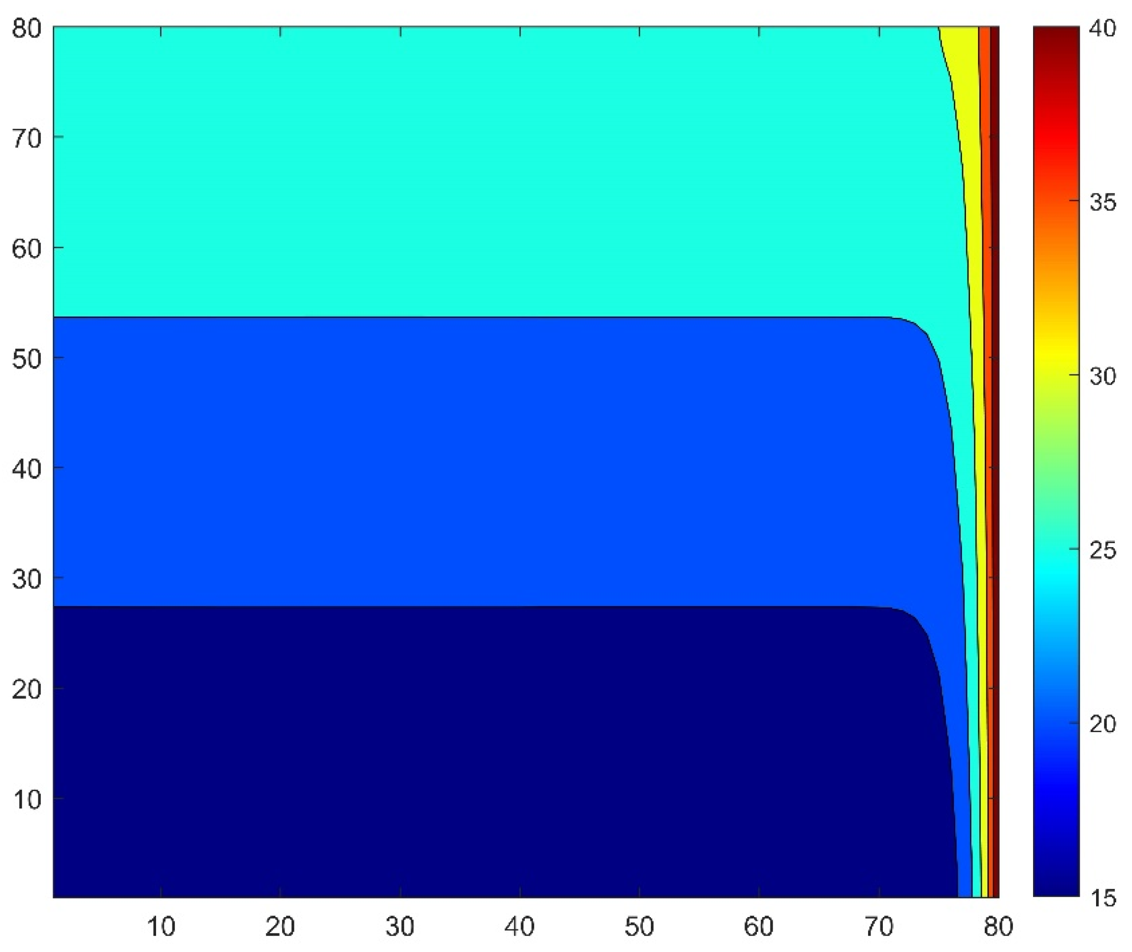
3.2. Brick Wall with Insulation, Dirichlet Boundary Conditions

We applied the sinusoidal initial and Dirichlet boundary condition of the point I for the multilayer wall with t_fin = 10,000. As it was mentioned above, the reference solution was provided by Heun’s method. The errors are plotted for equidistant and non-equidistant mesh in Figure 9 and Figure 10. We also plotted the final temperatures in the middle horizontal line of the wall for the reference solution and also for the LH method with quite a large time step size in Figure 11. One can now visualize the effect of the insulator (slower decrease of the temperature) and also see that the LH method is accurate for this large time step size.

One can see that now there are no residual errors. The reason for this is that the reference solution uses the same space discretization as the examined methods, thus this error disappears when the difference of the solutions is calculated as in Equation (16).

We observed that if we apply the insulator or go from equidistant mesh to increasingly non-equidistant meshes (both increase the stiffness), the OOEH method loses its advantage and the LH method will be the most accurate among the unconditionally stable methods. On the other hand, for very small time step sizes, Heun’s method is extremely accurate. However, this extent of accuracy is redundant in building energetics and in most other fields of engineering. Actually, this is one of the definitions of stiffness: “The step size is dictated by the stability requirements rather than the accuracy requirements” [46]. We stress again that this quoted sentence holds for the mainstream explicit methods, but it is not valid for the unconditionally stable methods, as one can see in the figures.

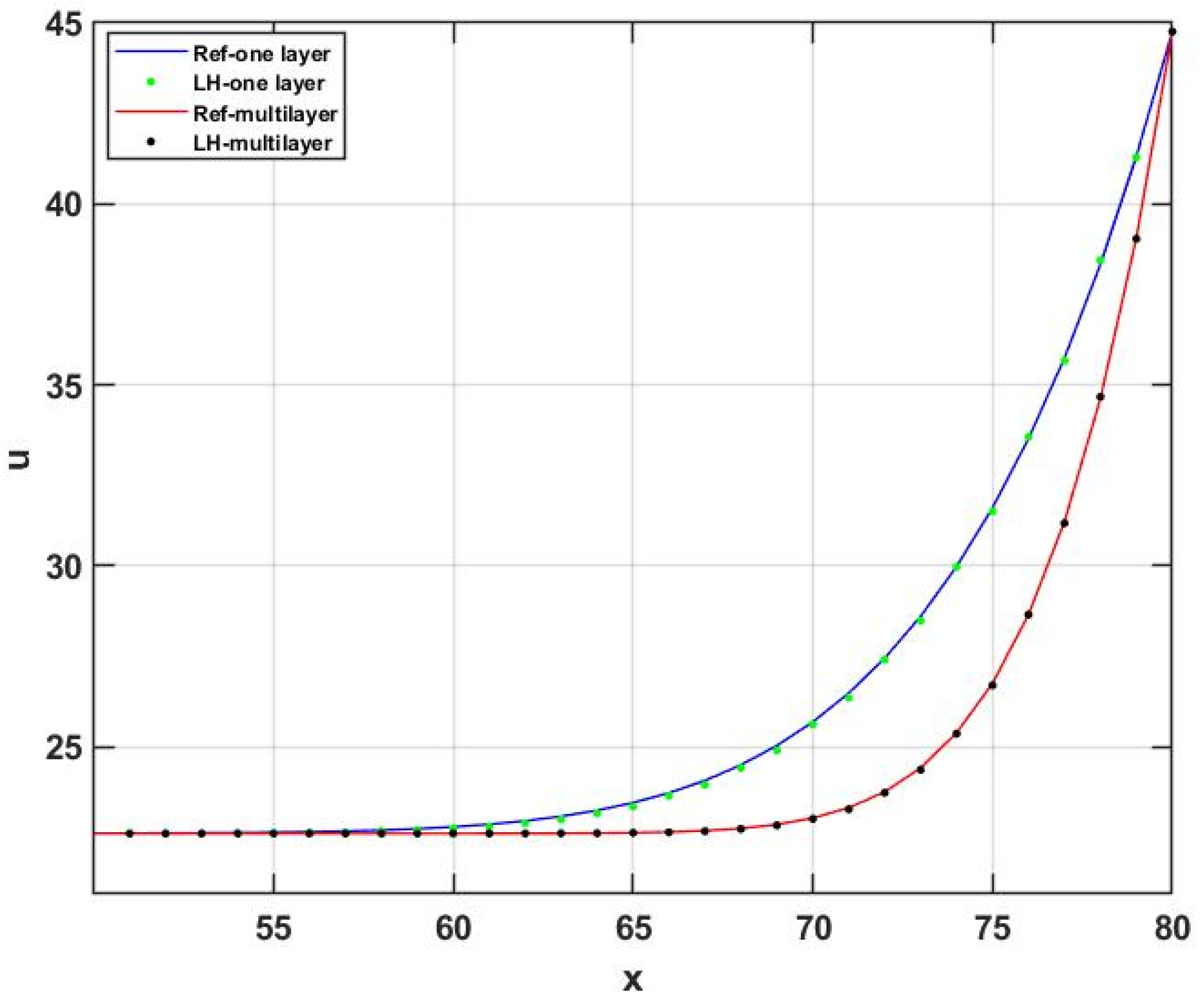
3.3. Realistic Case with Nontrivial Boundary Conditions

In this subsection, the initial condition is a linear function of space, while the boundary conditions are complicated as it is written in point II. The Neumann boundary conditions for upper and lower boundaries are implemented by setting the appropriate resistances to infinity, implying that the matrix elements describing heat transfer through the boundary vanish. First, we perform the simulation for the one-layer wall for two different grids (equidistant and gradual change in both directions), and only then for the insulated wall.

In Figure 12, we present the maximum errors for a one-layer wall with the equidistant mesh, while the temperature distribution contour is shown in Figure 13. For the non-equidistant mesh, the maximum errors and the energy-errors are presented in Figure 14 and Figure 15, respectively. The maximum and the energy error curves behave very similarly, the most significant change is that now the SH method performs better in terms of energy than the DF and the OOEH methods.

Let us now show the results for the multi-layer case. The maximum errors and the final temperature contours are presented in Figure 16 and Figure 17 in the case of the equidistant mesh. For the non-equidistant mesh, the maximum and energy errors are shown in Figure 18 and Figure 19, while the right-side temperature profile at medium height can be seen in Figure 20. From the figures it is evident that the LH method can easily cope with this complicated heat-conduction problem as well. One can also observe that the heat from the outer side of the insulator penetrates more slowly into the wall in the case of the insulated wall.

4. Discussion, Summary, and Future Plans

We numerically studied transient heat conduction in a two-dimensional wall with and without insulation. For this purpose, we applied eight recently invented and four old explicit and stable algorithms and the well-known Heun method.

For verification, an analytical solution of the heat equation was used with one equidistant and five non-equidistant grids but in the case of homogeneous material properties (one layer, brick only). Then, we examined the insulated wall using the same equidistant and non-equidistant grids. The boundary condition depended on space on the brick side of the wall and changes in time on the insulator side of the wall. All of the methods used are confirmed to be convergent, but their performance is not the same and depends on the circumstances.

The advantages and disadvantages of the methods are the following:

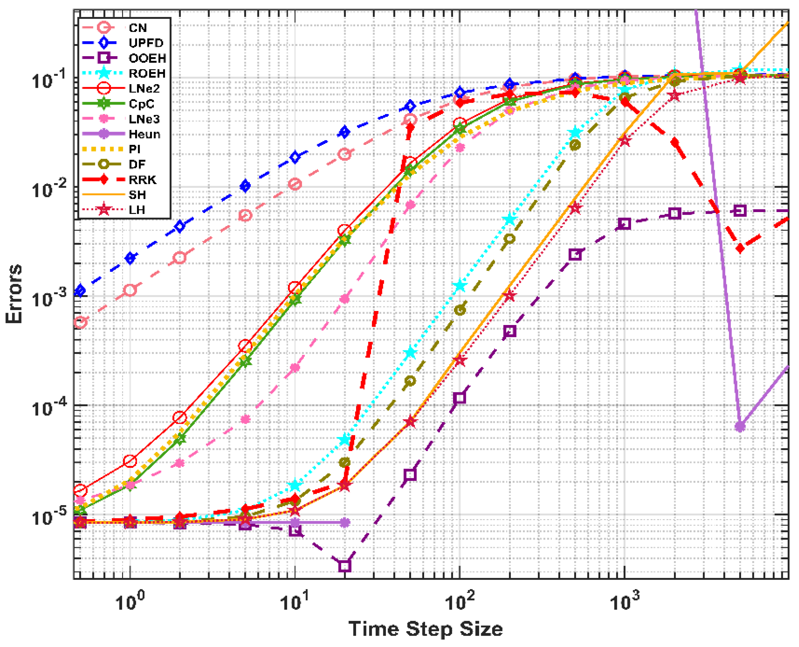
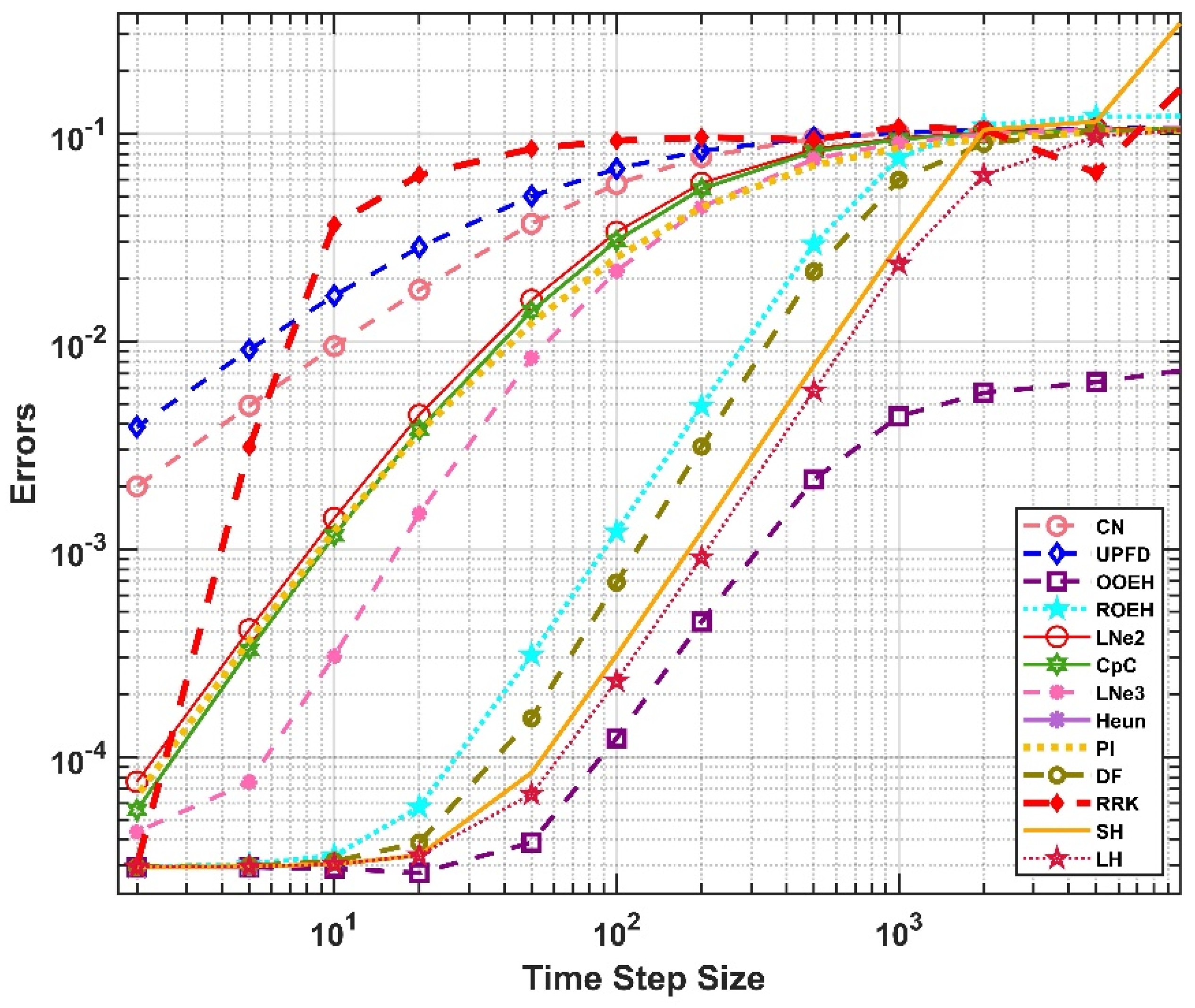
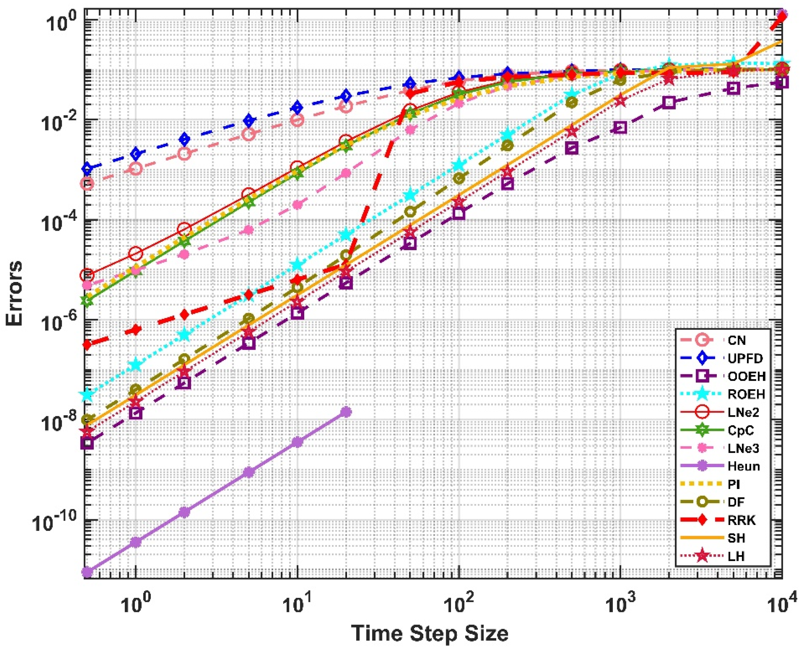
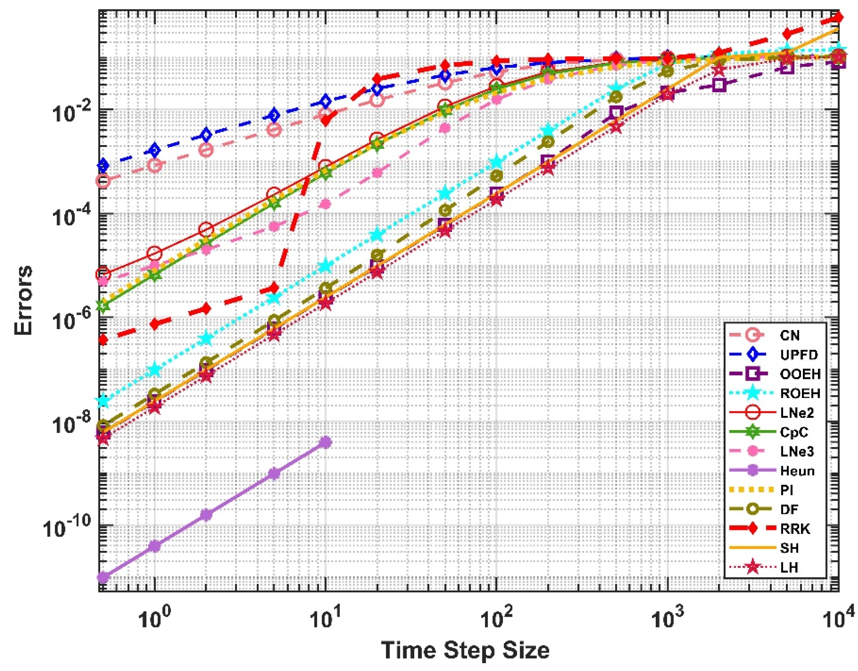
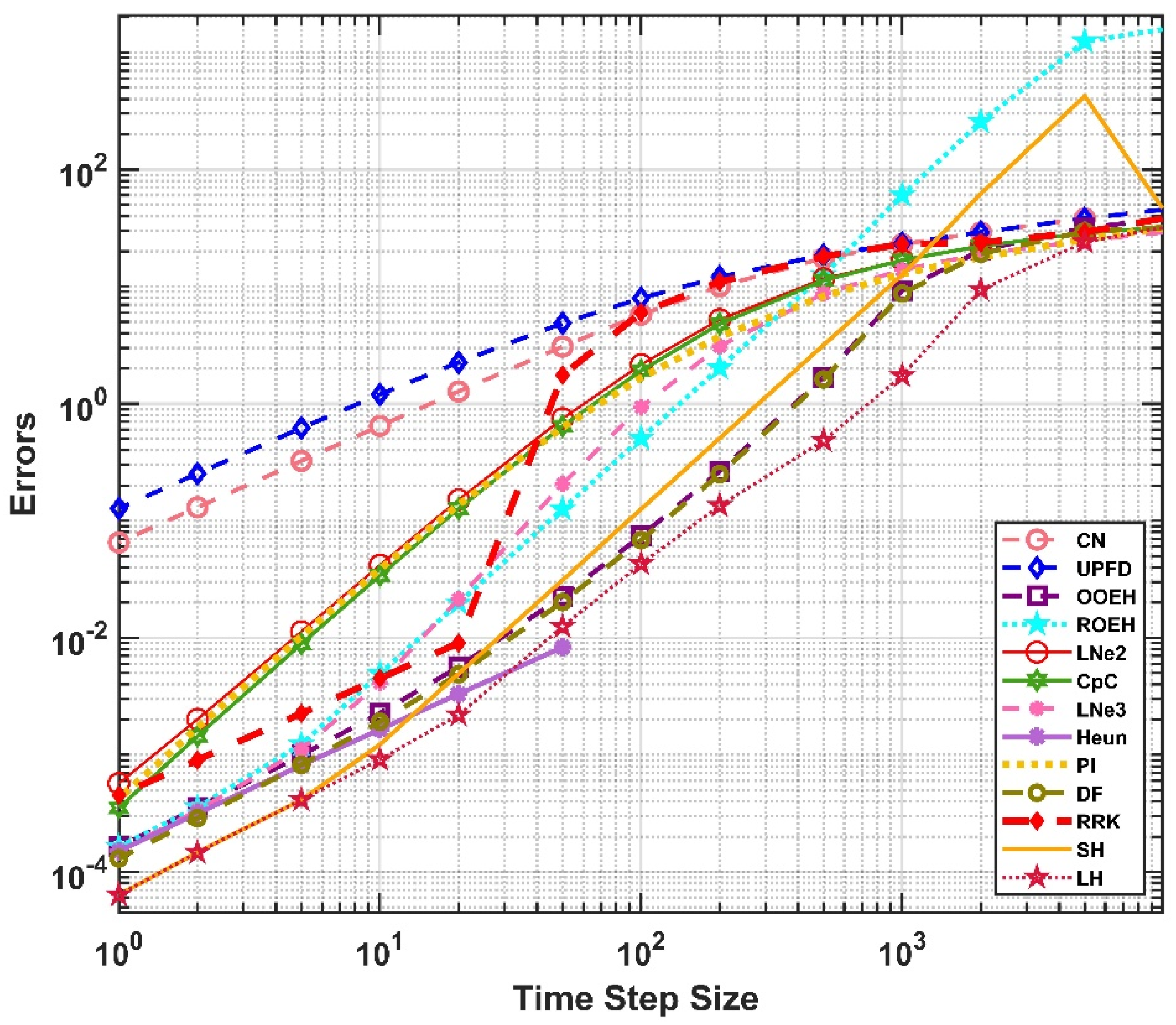
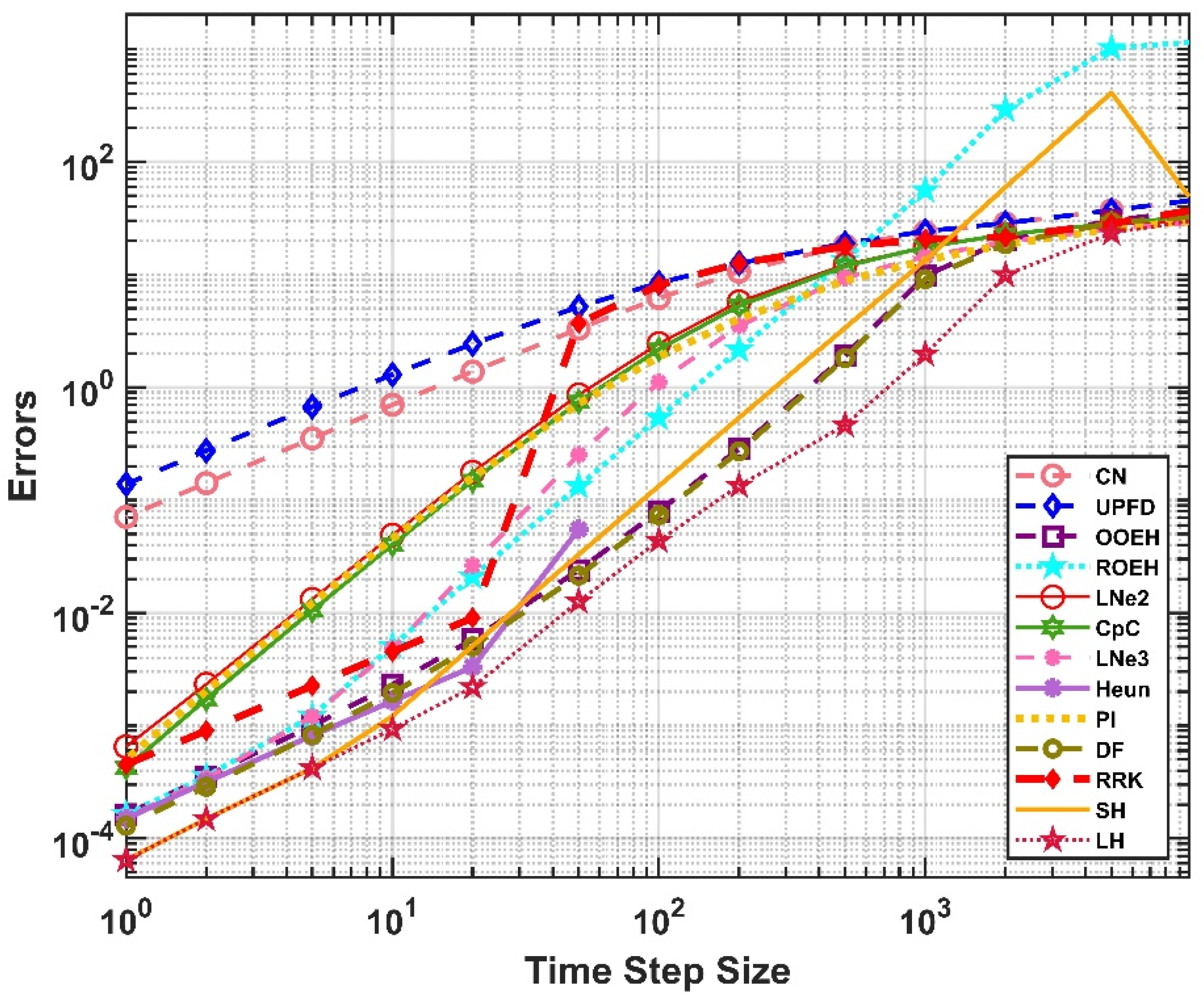
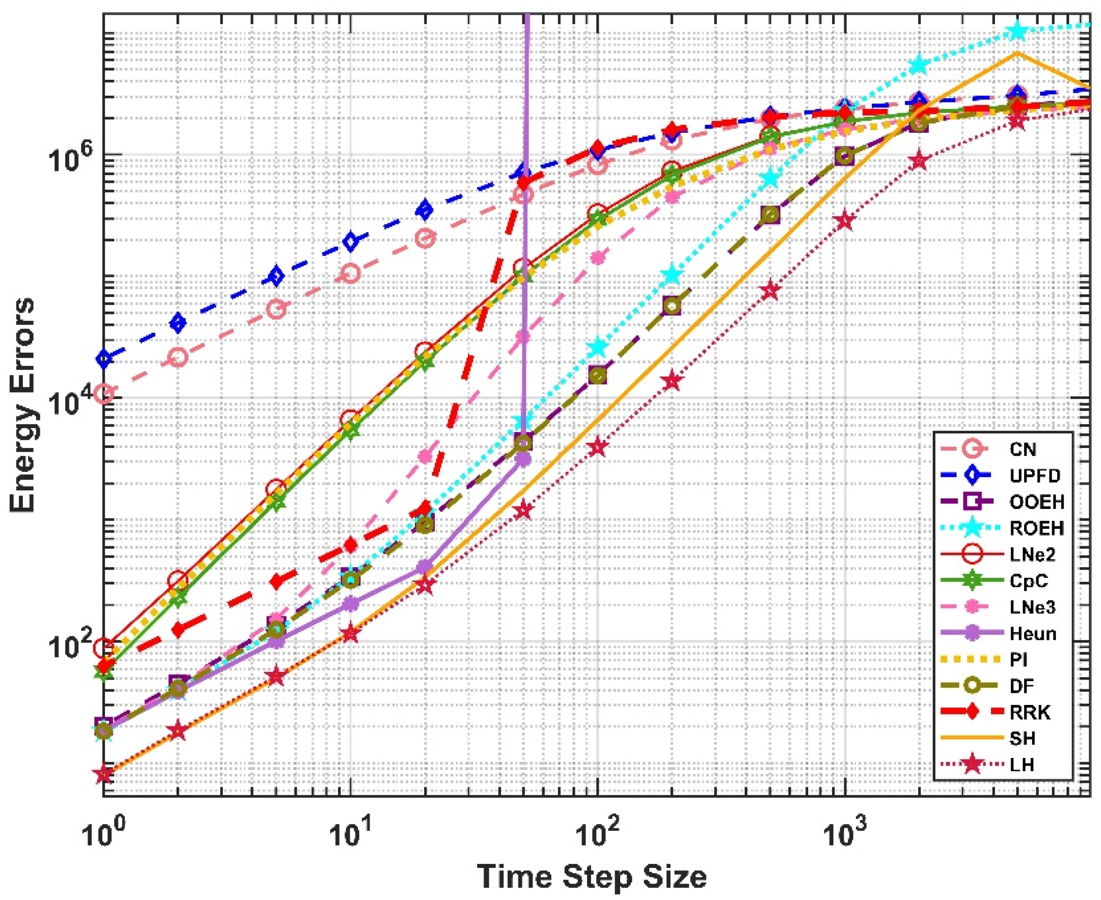
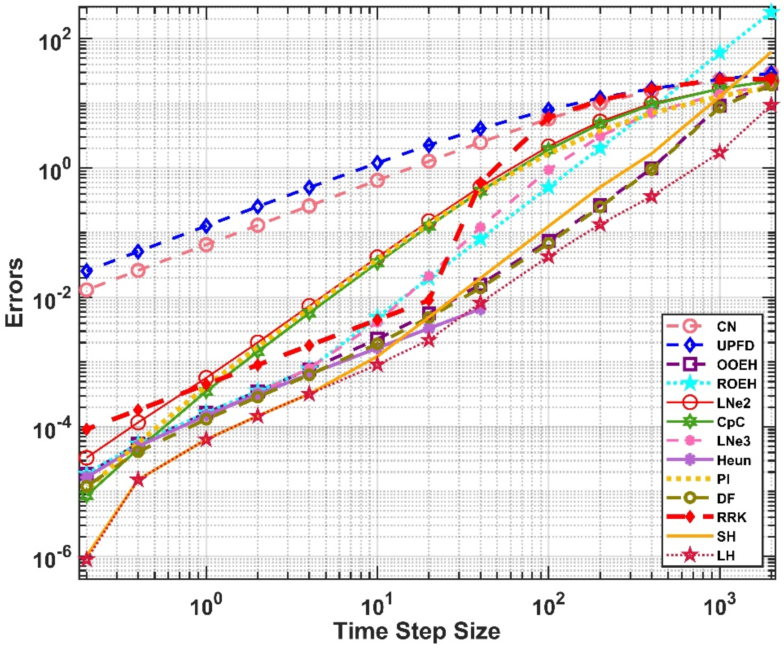
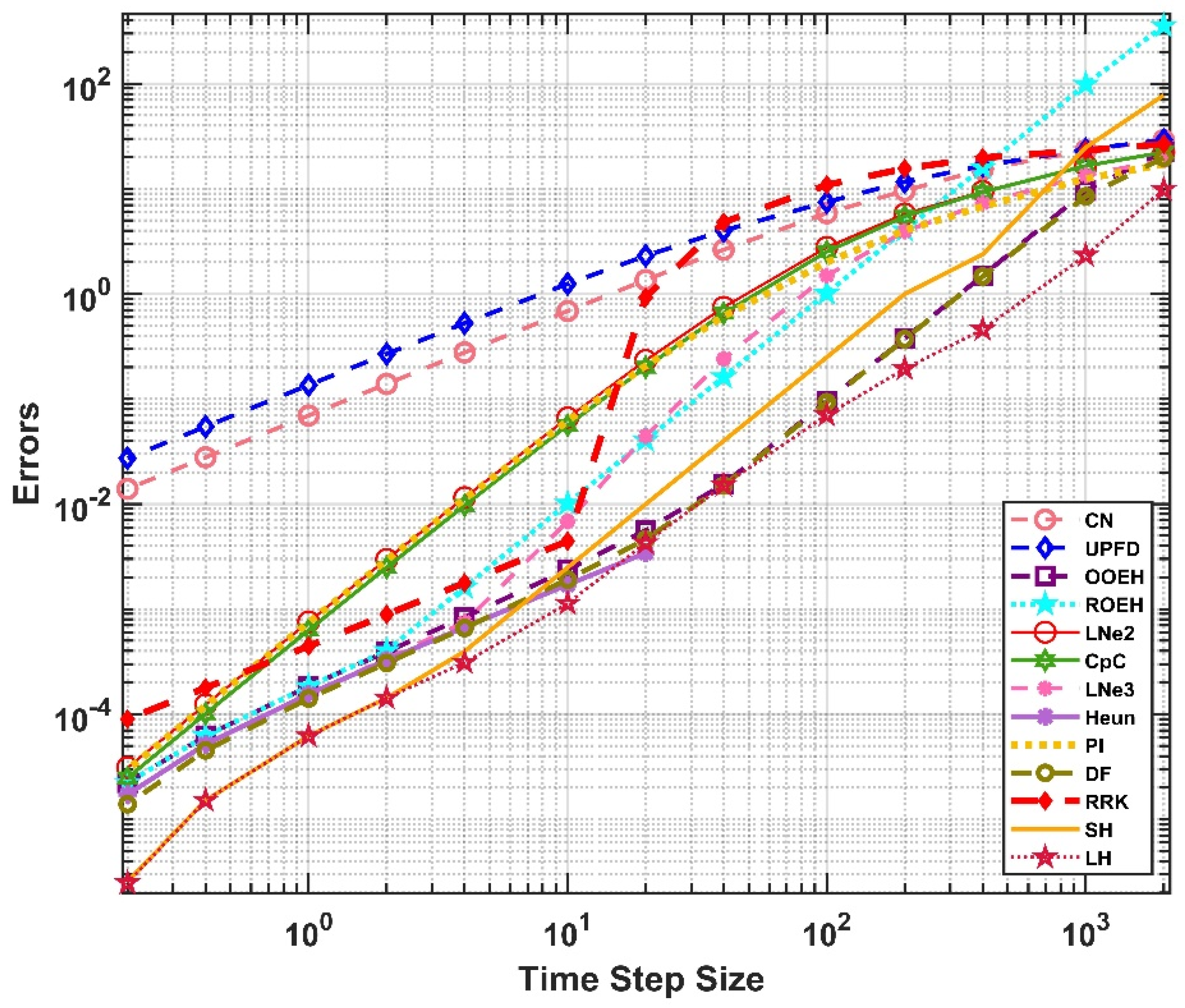
• The CNe and the UPFD are first order, thus not very accurate, all other methods are second order. Nevertheless, the RRK behaves as a first-order method for large and medium time step sizes.
• In the case of uniform (non-stiff) problems, the OOEH method is the most accurate for large and medium time step sizes. However, if stiffness increases, it can produce larger errors for large time step sizes. On the other hand, the LH always produces acceptable errors, and, usually, it is the most accurate for stiff systems.
• Heun’s method is only conditionally stable and was divergent for most of the time step sizes used, while all other methods are unconditionally stable.
• The CNe, the UPFD, the LNe2 and LNe3, and the CpC are positivity preserving for arbitrary time step size, all others are not. However, it implies that for medium and small time step sizes they are the least accurate.
• The hopscotch methods (OOEH, ROEH, SH, and LH) need a special bipartite grid. However, they do not require storing another copy of the array for the temperature, even temporarily, so they have minimal memory requirements. Other methods require the storage at least one extra array with the same number of elements as the array variable for the temperature.
• The level of generalizability of the methods is different. For example, the RRK and Heun’s methods are in principle completely general, so they can handle any modification of the original heat-equation. The UPFD and the pseudo-implicit methods can handle convection and reaction terms quite well, while some other methods have been adapted until now only to the cases of constant source terms and/or Fisher-type reaction terms besides the diffusion term. We note that the LH method has been successfully applied to the Kardar-Parisi-Zhang equation [47] as well.
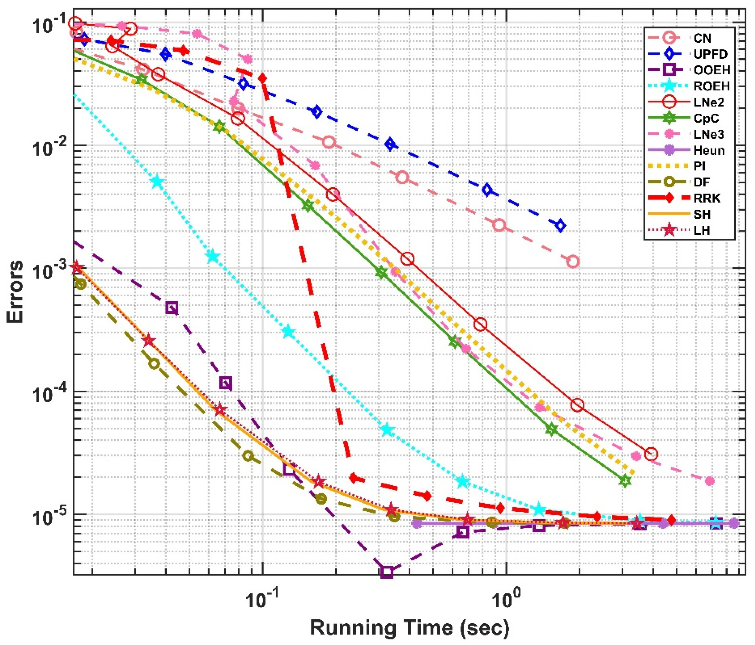
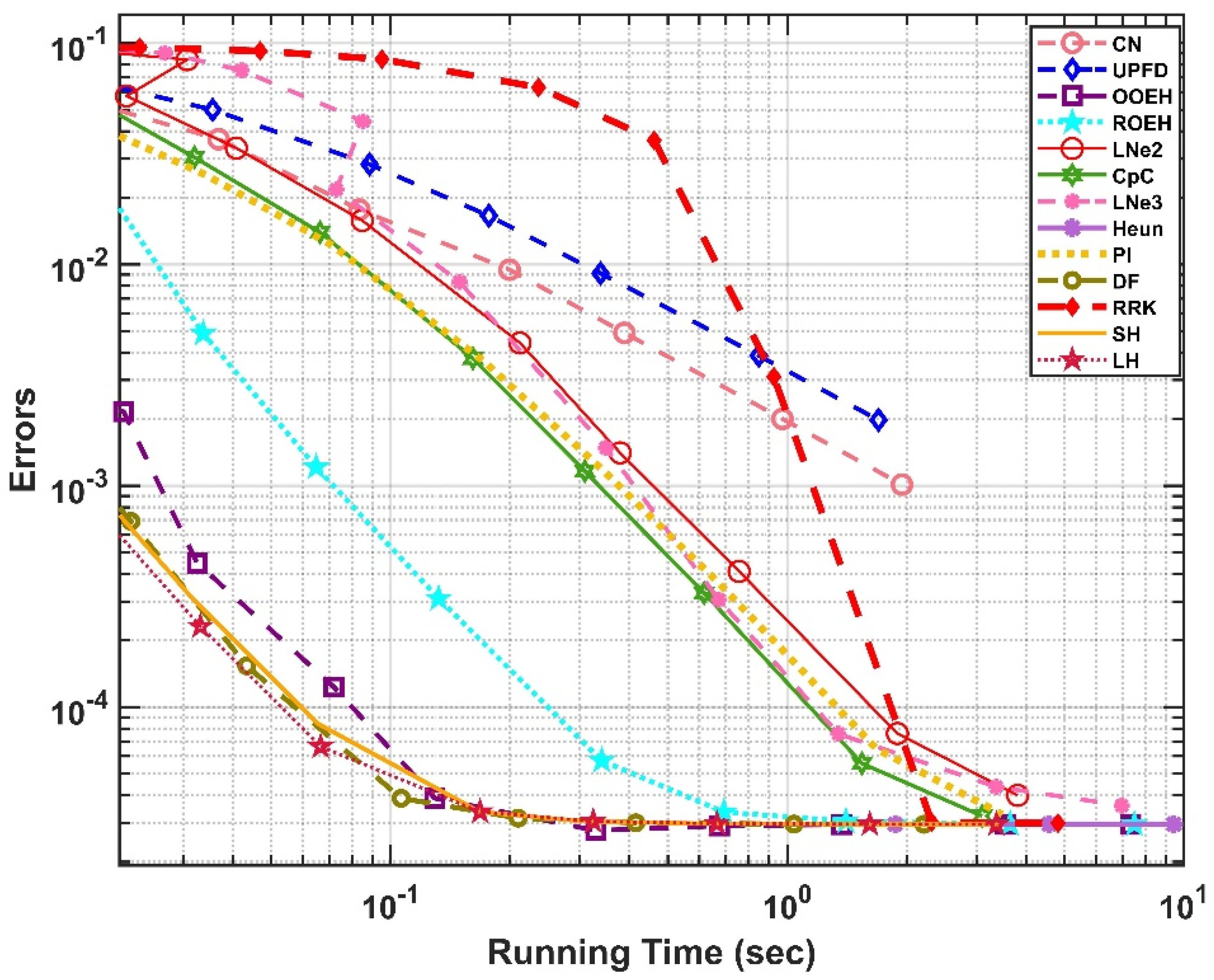
• The CNe, UPFD, OOEH, ROEH, DF, SH, and LH methods require only one calculation of the new temperature values of any cells in any given time step, so they are the fastest. The LNe2, CpC, Heun, PI, and RRK methods require two calculations while the LNe3 needs three calculations per cell per time step, thus it is roughly three times slower than, for example, the CNe method.
• DF is a two-step method; it needs to be started by another method.

To conclude, we can suggest using the OOEH or maybe the LH method in the case of homogeneous material properties and an equidistant grid, while in other cases the LH and maybe the SH and the DF algorithms can be proposed. All of them give quite accurate results with orders of magnitude larger time step size, thus they are much faster than the standard explicit methods stricken by instability. However, if unconditional positivity is crucial, the LNe3 method should be used to simulate heat conduction.

In the immediate future, we are going to adapt the most successful methods (especially the LH and the OOEH) to cases where there is heat transfer by convection and radiation as well. We plan to compare the results and the running times of our methods and that of appropriate commercial software, e.g., ANSYS Fluent. In the next step, we would like to examine nonlinear heat conduction, i.e., when the coefficients themselves depend on the temperature, and validate the results via real physical experiments. Then, we will be ready to apply the methods to real-life engineering problems, most importantly smart walls envelope, the use of phase change material (PCM), or study thermal bridges in buildings to increase energy efficiency. We will also work on the parallelization of the new algorithms, which we think can be done fairly straightforwardly due to the explicit nature of the algorithms.

References

1. Kusuda, T. Fundamentals of building heat transfer. J. Res. Natl. Bur. Stand. 1977, 82, 97. [Google Scholar] [CrossRef] [PubMed]
2. Li, T.; Xia, J.; Chin, C.S.; Song, P. Investigation of the Thermal Performance of Lightweight Assembled Exterior Wall Panel (LAEWP) with Stud Connections. Buildings 2022, 12, 473. [Google Scholar] [CrossRef]
3. Barna, I.F.; Mátyás, L. General Self-Similar Solutions of Diffusion Equation and Related Constructions. Rom. J. Phys. 2022, 67, 101. [Google Scholar]
4. Lienhard, J.H., IV; Lienhard, J.H., V. A Heat Transfer Textbook, 4th ed.; Phlogiston Press: Cambridge, MA, USA, 2017; ISBN 9780971383524. [Google Scholar]
5. Savović, S.; Djordjevich, A. Numerical solution of diffusion equation describing the flow of radon through concrete. Appl. Radiat. Isot. 2008, 66, 552–555. Available online: https://www.sciencedirect.com/science/article/pii/S0969804307002874 (accessed on 13 June 2022). [CrossRef]
6. Suárez-Carreño, F.; Rosales-Romero, L. Convergency and stability of explicit and implicit schemes in the simulation of the heat equation. Appl. Sci. 2021, 11, 4468. [Google Scholar] [CrossRef]
7. Haq, S.; Ali, I. Approximate solution of two-dimensional Sobolev equation using a mixed Lucas and Fibonacci polynomials. Eng. Comput. 2021. Available online: https://link.springer.com/article/10.1007/s00366-021-01327-5 (accessed on 13 June 2022). [CrossRef]
8. Lima, S.A.; Kamrujjaman, M.; Islam, M.S. Numerical solution of convection-diffusion-reaction equations by a finite element method with error correlation. AIP Adv. 2021, 11, 085225. [Google Scholar] [CrossRef]
9. Ivanovic, M.; Svicevic, M.; Savovic, S. Numerical solution of Stefan problem with variable space grid method based on mixed finite element/ finite difference approach. Int. J. Numer. Methods Heat Fluid Flow 2017, 27, 2682–2695. [Google Scholar] [CrossRef]
10. Zhang, J.; Zhao, C. Sharp error estimate of BDF2 scheme with variable time steps for molecular beam expitaxial models without slop selection. J. Math. 2021, 41, 1–19. [Google Scholar]
11. Amoah-Mensah, J.; Boateng, F.O.; Bonsu, K. Numerical solution to parabolic PDE using implicit finite difference approach. Math. Theory Model. 2016, 6, 74–84. [Google Scholar]
12. Mbroh, N.A.; Munyakazi, J.B. A robust numerical scheme for singularly perturbed parabolic reaction-diffusion problems via the method of lines. Int. J. Comput. Math. 2021, 2021, 1–25. [Google Scholar] [CrossRef]
13. Aminikhah, H.; Alavi, J. An efficient B-spline difference method for solving system of nonlinear parabolic PDEs. SeMA J. 2018, 75, 335–348. [Google Scholar] [CrossRef]
14. Ali, I.; Haq, S.; Nisar, K.S.; Arifeen, S.U. Numerical study of 1D and 2D advection-diffusion-reaction equations using Lucas and Fibonacci polynomials. Arab. J. Math. 2021, 10, 513–526. [Google Scholar] [CrossRef]
15. Singh, M.K.; Rajput, S.; Singh, R.K. Study of 2D contaminant transport with depth varying input source in a groundwater reservoir. Water Sci. Technol. Water Supply 2021, 21, 1464–1480. [Google Scholar] [CrossRef]
16. Haq, S.; Hussain, M.; Ghafoor, A. A computational study of variable coefficients fractional advection–diffusion–reaction equations via implicit meshless spectral algorithm. Eng. Comput. 2020, 36, 1243–1263. Available online: https://link.springer.com/article/10.1007/s00366-019-00760-x (accessed on 13 June 2022). [CrossRef]
17. Reguly, I.Z.; Mudalige, G.R. Productivity, performance, and portability for computational fluid dynamics applications. Comput. Fluids 2020, 199, 104425. [Google Scholar] [CrossRef]
18. Gagliardi, F.; Moreto, M.; Olivieri, M.; Valero, M. The international race towards Exascale in Europe. CCF Trans. High Perform. Comput. 2019, 1, 3–13. [Google Scholar] [CrossRef] [Green Version]
19. Appadu, A.R. Performance of UPFD scheme under some different regimes of advection, diffusion and reaction. Int. J. Numer. Methods Heat Fluid Flow 2017, 27, 1412–1429. [Google Scholar] [CrossRef] [Green Version]
20. Karahan, H. Unconditional stable explicit finite difference technique for the advection-diffusion equation using spreadsheets. Adv. Eng. Softw. 2007, 38, 80–86. [Google Scholar] [CrossRef]
21. Sanjaya, F.; Mungkasi, S. A simple but accurate explicit finite difference method for the advection-diffusion equation. J. Phys. Conf. Ser. 2017, 909, 1–5. [Google Scholar] [CrossRef]
22. Pourghanbar, S.; Manafian, J.; Ranjbar, M.; Aliyeva, A.; Gasimov, Y.S. An efficient alternating direction explicit method for solving a nonlinear partial differential Equation. Math. Probl. Eng. 2020, 2020, 1–12. [Google Scholar] [CrossRef]
23. Harley, C. Hopscotch method: The numerical solution of the Frank-Kamenetskii partial differential equation. Appl. Math. Comput. 2010, 217, 4065–4075. [Google Scholar] [CrossRef]
24. Al-Bayati, A.Y.; Manaa, S.A.; Al-Rozbayani, A.M. Comparison of Finite Difference Solution Methods for Reaction Diffusion System in Two Dimensions. AL-Rafidain J. Comput. Sci. Math. 2011, 8, 21–36. [Google Scholar] [CrossRef] [Green Version]
25. Nwaigwe, C. An Unconditionally Stable Scheme for Two-Dimensional Convection-Diffusion-Reaction Equations. 2022. Available online: https://www.researchgate.net/publication/357606287_An_Unconditionally_Stable_Scheme_for_Two-Dimensional_Convection-Diffusion-Reaction_Equations (accessed on 13 June 2022).
26. Savović, S.; Drljača, B.; Djordjevich, A. A comparative study of two different finite difference methods for solving advection–diffusion reaction equation for modeling exponential traveling wave in heat and mass transfer processes. Ric. Mat. 2021, 70, 2. [Google Scholar] [CrossRef]
27. Kovács, E.; Gilicz, A. New stable method to solve heat conduction problems in extremely large systems. Des. Mach. Struct. 2018, 8, 30–38. [Google Scholar]
28. Kovács, E. New Stable, Explicit, First Order Method to Solve the Heat Conduction Equation. J. Comput. Appl. Mech. 2020, 15, 3–13. Available online: http://www.mech.uni-miskolc.hu/jcam/author_card.php?author_id=375 (accessed on 13 June 2022). [CrossRef]
29. Issa, O. New explicit algorithm based on the asymmetric hopscotch structure to solve the heat conduction equation. Multidiszcip. Tudományok 2021, 11, 233–244. [Google Scholar]
30. Saleh, M.; Nagy, Á.; Kovács, E. Part 1: Construction and investigation of new numerical algorithms for the heat equation. Multidiszcip. Tudományok 2020, 10, 323–338. [Google Scholar] [CrossRef]
31. Saleh, M.; Nagy, Á.; Kovács, E. Part 2: Construction and investigation of new numerical algorithms for the heat equation. Multidiszcip. Tudományok 2020, 10, 339–348. [Google Scholar] [CrossRef]
32. Saleh, M.; Nagy, Á.; Kovács, E. Part 3: Construction and investigation of new numerical algorithms for the heat equation. Multidiszcip. Tudományok 2020, 10, 349–360. [Google Scholar] [CrossRef]
33. Nagy, Á.; Saleh, M.; Omle, I.; Kareem, H.; Kovács, E. New stable, explicit, shifted-hopscotch algorithms for the heat equation. Math. Comput. Appl. 2021, 26, 61. Available online: https://www.mdpi.com/2297-8747/26/3/61/htm (accessed on 13 June 2022). [CrossRef]
34. Nagy, Á.; Omle, I.; Kareem, H.; Kovács, E.; Barna, I.F.; Bognar, G. Stable, Explicit, Leapfrog-Hopscotch Algorithms for the Diffusion Equation. Computation 2021, 9, 92. [Google Scholar] [CrossRef]
35. Kovács, E.; Nagy, Á.; Saleh, M. A set of new stable, explicit, second order schemes for the non-stationary heat conduction equation. Mathematics 2021, 9, 2284. Available online: https://www.mdpi.com/2227-7390/9/18/2284 (accessed on 3 November 2021). [CrossRef]
36. Jalghaf, H.K.; Kovács, E.; Majár, J.; Nagy, Á.; Askar, A.H. Explicit stable finite difference methods for diffusion-reaction type equations. Mathematics 2021, 9, 3308. [Google Scholar] [CrossRef]
37. Munka, M.; Pápay, J. 4D Numerical Modeling of Petroleum Reservoir Recovery; Akadémiai Kiadó: Budapest, Hungary, 2001; ISBN 9630578433. [Google Scholar]
38. Kovács, E. A class of new stable, explicit methods to solve the non-stationary heat equation. Numer. Methods Partial Differ. Equ. 2020, 37, 2469–2489. [Google Scholar] [CrossRef]
39. Holmes, M.H. Introduction to Numerical Methods in Differential Equations; Springer: New York, NY, USA, 2007; ISBN 9780387308913. [Google Scholar]
40. Gourlay, A.R.; McGuire, G.R. General Hopscotch Algorithm for the Numerical Solution of Partial Differential Equations. IMA J. Appl. Math. 1971, 7, 216–227. [Google Scholar] [CrossRef]
41. Heun’s Method—Wikipedia. Available online: https://en.wikipedia.org/wiki/Heun%27s_method (accessed on 30 July 2021).
42. Hirsch, C. Numerical Computation of Internal and External Flows, Volume 1: Fundamentals of Numerical Discretization; Wiley: Hoboken, NJ, USA, 1988. [Google Scholar]
43. Sottas, G. Rational Runge-Kutta methods are not suitable for stiff systems of ODEs. J. Comput. Appl. Math. 1984, 10, 169–174. [Google Scholar] [CrossRef] [Green Version]
44. Kovács, E.; Nagy, Á.; Saleh, M. A New Stable, Explicit, Third-Order Method for Diffusion-Type Problems. Adv. Theory Simul. 2022, 5, 2100600. [Google Scholar] [CrossRef]
45. Iserles, A. A First Course in the Numerical Analysis of Differential Equations; Cambridge University Press: Cambridge, UK, 2009; ISBN 9788490225370. [Google Scholar]
46. Bastani, M.; Salkuyeh, D.K. A highly accurate method to solve Fisher’s equation. Pramana-J. Phys. 2012, 78, 335–346. [Google Scholar] [CrossRef]
47. Sayfidinov, O.; Bognár, G.; Kovács, E. Solution of the 1D KPZ Equation by Explicit Methods. Symmetry 2022, 14, 699. [Google Scholar] [CrossRef]
Figure 1. (A) One-layer wall, (B) and (C) wall with insulator.
Buildings 12 00824 g001
Figure 2. (A) Abrupt change. (B) Gradual change in the x direction.
Buildings 12 00824 g002
Figure 5. The maximum errors as a function of the time step size Δ t for the 13 examined methods in the case of an equidistant mesh.
Buildings 12 00824 g005
Figure 6. The maximum errors as a function of the time step size Δ t for the abrupt change in the x-direction and gradual change in the z-direction.
Buildings 12 00824 g006
Figure 7. The maximum errors as a function of the running time for the 13 examined methods in the case of an equidistant mesh.
Buildings 12 00824 g007
Figure 8. The maximum errors as a function of the running time for the abrupt change in the x-direction and gradual change in the z-direction.
Buildings 12 00824 g008
Figure 9. The maximum errors as a function of the time step size Δ t for equidistant mesh.
Buildings 12 00824 g009
Figure 10. The L errors as a function of the time step size Δ t in case of abrupt change in the x-direction and gradual change in the z-direction.
Buildings 12 00824 g010
Figure 11. The temperature as a function of the cell index in the x direction at the middle row ( z 0.5 ) in the case of the reference solution (Ref) and the leapfrog-hopscotch (LH) method for Δ t = 400 in the case of the one-layer wall and the insulated wall using an equidistant grid.
Buildings 12 00824 g011
Figure 12. The L errors as a function of the time step size Δ t for the equidistant mesh.
Buildings 12 00824 g012
Figure 13. The temperature distribution contour for the equidistant mesh at the final time.
Buildings 12 00824 g013
Figure 14. The L errors as a function of the time step size Δ t for the non-equidistant mesh.
Buildings 12 00824 g014
Figure 15. The energy errors defined in (17) as a function of the time step size Δ t for the non-equidistant mesh.
Buildings 12 00824 g015
Figure 16. The maximum errors as a function of the time step size Δ t for the equidistant mesh for a wall with insulation.
Buildings 12 00824 g016
Figure 17. The temperature distribution contour for equidistant mesh in the case of a wall with insulation.
Buildings 12 00824 g017
Figure 18. The maximum errors as a function of the time step size Δ t for the non-equidistant mesh for a wall with insulation.
Buildings 12 00824 g018
Figure 19. The energy errors as a function of the time step size Δ t for the non-equidistant mesh for a wall with insulation.
Buildings 12 00824 g019
Figure 20. The temperature as a function of the cell index in the x direction at the middle row ( z 0.5 ) in the case of the reference solution (Ref) and the leapfrog-hopscotch (LH) method for Δ t = 400 in the case of the one-layer wall and the insulated wall using an equidistant grid.
Buildings 12 00824 g020