Abstract
This paper presented a Computational Fluid Dynamics (CFD) study on the relationship between skyline quantitative factors and the wind environment. At present, most researches on skyline revealed the changes of skyline quantitative factors on the aesthetic degrees but neglected the influence of the factors on the outdoor wind environment. This paper addresses the gap in using the changing factors for the prediction of outdoor wind speed. It provides a standardized range for aesthetic degrees in the comfortable range of the wind environment and an exact relationship between the factors and the wind environment. To validate the effectiveness of the proposed approach, a case study is undertaken on the existing skyline of Qianjiang New City in Hangzhou and extracts the following three skyline quantitative factors in skyline contour: contour tortuosity, building undulation, and skyline rhythm index. The result shows that the proposed range and relationship are ready to provide a quantitative understanding of the skyline under outdoor wind conditions.
1. Introduction
The skyline aesthetic degrees have led to the development of the aesthetic metrics of the skyline. Researchers have proposed different quantification factors to control the morphological changes of skylines. There are the following three aspects to constructing an aesthetic evaluation model of the skyline: spatial form, skyline contour, and architectural form. Spatial openness index and space level evaluate the urban space in quantitative [1,2]. Contour tortuosity, building undulation, and the skyline rhythm index propose a quantitative description of urban skyline form from visual impact [3,4]. Additionally, turn in the outline of the roof and building width for emphasis on the architectural attribution [5]. To evaluate the aesthetic degree of the skyline, researchers have combined public research with quantitative analysis to evaluate aesthetic preferences more objectively. According to the use of building images of different complexity degrees in the investigation to obtain a level of pleasure in people, a positive relationship between building/skyline contour complexity and people’s pleasure is proved [6,7,8].
The changes in architectural form cause not only changes in skyline form but also differences in microclimate. The wind environment, as an important part of the microclimate, is a research priority for researchers today. There is a paucity of studies that research the differences in their wind environments from skyline morphology. Most researchers have focused on the relationship between the layout of the architectural complex at different scales and the outdoor wind environment.
For city-wide scale urban spatial form, the studies are mostly on the influence of large scale, high density, typical high-rise architectural complexes with outdoor wind environments, such as urban centers, high-tech districts, etc. Researchers have used wind environment simulations of typical high-rise building complexes to provide suggestions for improving uncomfortable building layouts to reduce safety risks [9,10,11]. There also exists work which explores the relationship between wind speed and the building density, volume rate, average building height, etc. [12,13]. In general, city-wide scale researches can provide directional guidance for the outdoor wind environment. However, the scope of the studies is too large, and their forms are complex. It is difficult to summarize the variation to guide the morphological changes from the perspective of wind environment optimization.
For eeso-micro-scale urban spatial form, it is the typical layout of architectural complexes, such as neighborhood units, several residential areas, central business districts (CBD), etc. Researchers have researched outdoor wind environments in monolayouts, actual layouts, and ideal layouts. Some researchers have studied the regularity between the plan, height, and the number of monolayout openings and wind speed to induce the climatic environment [14,15,16,17]. Other researchers provide certain suggestions for optimizing the building forms by studying the layout of residential or office buildings in actual and ideal layouts with outdoor wind environments to guide the ventilation and morphology strategies [18,19,20,21,22,23,24,25,26]. Due to its small scale, the optimization suggestions between the layouts and the wind environment are more easily summarized. However, the eeso-micro scale of the studies is the parts of the skyline, which are usually residential or office areas. Additionally, the urban construction factors of the skyline contain both residential and office areas. In general, there is a lack of outdoor wind environment studies in the skyline scale range.
Therefore, the skyline is a special area of the city. There is a relative lack of research on the outdoor wind environment on its scale. This study intends to take the skyline as the object of research and explore the correlation between the skyline’s quantitative factors and the outdoor wind environment. The aim is to pursue the double-optimal goal of aesthetic pleasure and physical comfort.
2. Materials and Methods
2.1. Evaluation Index
2.1.1. Evaluation Index of the Skyline Quantitative
- Contour tortuosity: it represents the wave of the skyline (Figure 1). The contour tortuosity is defined by Equation (1). is contour tortuosity of the whole skyline, is single band of contour tortuosity, is the sum of differences of each band between the low and high points, and refers to the horizontal distance of each band [27].
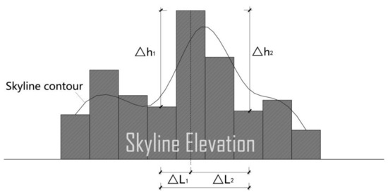 Figure 1. Contour tortuosity.
 - Building undulation: it represents the lengthwise rhythm of the skyline (Figure 2). It is calculated the percentage of elevation difference between the tallest building and the shortest building (except the podium) in all units according to each 100m horizontal distance as a unit. The building undulation is defined by Equation (2). is building undulation of the whole skyline, is the degree of unit building undulation, which means the difference between the highest building and the lowest building in every 100 m units [28].
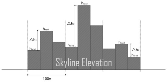 Figure 2. Building undulation.
 - Skyline rhythm index: it represents the transverse rhythm of the skyline (Figure 3). The contour whose elevation difference between adjacent buildings does not exceed 30 m is defined as a flattened contour, and vice versa as a fluctuation contour. The ratio of the flattened contour length to the total skyline length is calculated. The skyline rhythm index is defined by Equation (3). is skyline rhythm index of the whole skyline, is the length of flattened contour, and is the whole length of the skyline [28].
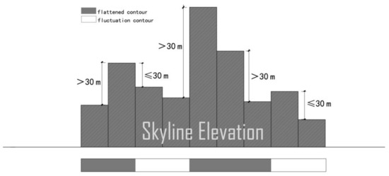 Figure 3. Skyline rhythm index.
2.1.2. Evaluation Index of the Wind Environment
- Wind speed ratio: it represents an index to evaluate the comfort level of wind environment comfort. The wind speed ratio is generated according to Equation (4). Rw is the wind speed ratio, Vs is the absolute value of wind speed at the measuring point at the pedestrian height, and v means the absolute value of initial wind speed at the pedestrian height. Previous studies have shown that the wind speed ratio is more comfortable for pedestrians in the range of 0.5–2.0 [29] (Table 1) The evaluation method of wind speed ratio is more objective and is used in current research. However, its disadvantage is that the evaluation of wind speed ratio is difficult to complete the detection of wind environment in the areas for different measuring points.
 Table 1. The standard of wind speed ratio comfort.
 - Therefore, researchers introduce the average wind speed ratio index to evaluate the regional wind environment. The overall ventilation level of urban scope is reflected by comparing the ratio of average wind speed at pedestrian height to initial wind speed. The average wind speed ratio is generated according to Equation (5). RM is the average wind speed ratio index, Vi is the absolute value of average wind speed at pedestrian height, vr is the absolute value of initial wind speed at the same height [30].
- Wind speed ratio dispersion: it is an important index to evaluate the stability of wind speed. The change in the wind speed is calculated to obtain the dispersion of each district’s wind speed. The high dispersion will cause the unstable distribution of wind speed [31]. Wind speed ratio dispersion is calculated according to Equation (6). is the wind speed ratio dispersion, n means the number of data, and is the average of all values.
2.2. Computational Fluid Dynamics Model
2.2.1. Study Area
Due to the large range of Qianjiang New City skyline in Hangzhou, the range was simplified by the observer’s horizontal viewing angle. With a human height of 1.65 m and a horizontal viewing angle of 120° (Figure 4), the width of the visual viewing field was calculated according to Equation (7). L is the width of the visual viewing field; D is the visual viewing range. Taking the width of Qiantang River 1000 m as the visual viewing range D, the width of the visual viewing field L was calculated as 3464 m. The lateral range was from Qingchun Road Tunnel to Wujiang Road [32].
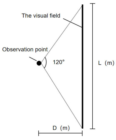
Figure 4.
The field of view for horizontal view.
As the visual range D was 1000m, the viewing range was such that the overall skyline could be seen (Table 2). Thus, the vertical range was the main skyline part of Qianjiang New City between Zhijiang Road and Fuchun Road. The outdoor wind environment simulation scope was the area between Zhijiang Road and Fuchun Road, from Qingchun Road Tunnel to Wugang Road (Figure 5).
Table 2.
Skyline hierarchical classification.
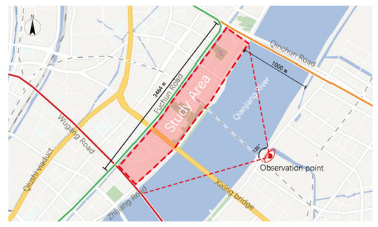
Figure 5.
Study area.
2.2.2. Skyline Model
To obtain the general plan in the research range, it was captured in the CAD mapper and simplified in AutoCAD. The height and morphology information of buildings was obtained in the field measurement and data collection. Then the skyline model was set up in Sketchup. The model in building details (such as the changes of roof, balcony et al.) could be ignored to improve the outdoor wind environment simulation more efficiently. Finally, a simplified model of Hangzhou Qianjiang New City skyline suitable for simulation was obtained (Figure 6).
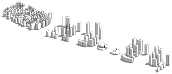
Figure 6.
Model of Simulation area.
2.2.3. Computational Domain
When the model was imported into Phoenics, the building coverage area was less than 3% of the whole calculation area. The radius within 5H, where H was the height of the main building, was the horizontal calculation domain while taking the target building as the center [33]. The calculation area above the buildings should be larger than 3H, so the size of the simulation area in this paper was 22,000 m × 6200 m × 600 m.
2.2.4. Boundary Conditions
In this study, the Reynolds-Averaged Navier–Stokes (RANS) with a standard k-ε turbulence model was used to calculate the airflow. To obtain better convergence and accuracy, the discrete scheme adopted the second-order wind scheme and 10−4 as the convergence basis [34]. Additionally, the time step was set as 1.
The velocity inlet boundary condition was set as the gradient wind with a given wind speed. The main wind direction in Hangzhou is southwest wind in summer and northwest wind in winter. But the dominant wind direction varies due to different geographical conditions. In the riverside area, the Qiantang River coast becomes a natural corridor for water vapor and power transmission because it is guided by southeast winds in summer [35]. And the Qianjiang New City area is also influenced by the transpiration of large water with southeast wind. Thus, the main wind direction in summer is southeast. The initial wind direction was set to southeast in summer and northwest in winter. The wind speed ratio was used for evaluation, and the wind speed of 10 m/s was used for simulation to make the results more intuitive.
Surface friction is generated when the airflow passes through roughness elements (Figure 7). Surface friction force impedes airflow near the ground, which leads to a reduction in wind speed. This friction gradually decreases in the vertical direction as the height of the ground increases until it disappears at a certain height. Then the gradient wind is created. It is defined by Equation (8). U(z) is the average wind speed at height Z, UG is the average wind speed at the standard height ZG and α is a parameter to describe the surface roughness [36] (Table 3).
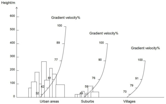
Figure 7.
Variation of gradient wind at different roughness.
Table 3.
Ground roughness index α and corresponding gradient wind height ZG.
Due to the effect of surface friction, the wind speed near the surface decreases with the height above the ground decreases. When it is 300–500 m above the ground, the wind speed will not be affected by the surface friction and the wind can flow freely under the effect of atmospheric gradient. The Qianjiang New City in Hangzhou was a high dense area with a Class D ground roughness. The simulation conditions were set as α = 0.30, = 450 m. Because there were no buildings on the outflow surface to influence the natural flow of wind speed, the outflow interface was set as a natural outflow boundary. The top and sides of the calculation area were flow boundaries. They set as free-slip wall. The ground was fixed, and it was set as no-slip wall (Figure 8) [37].
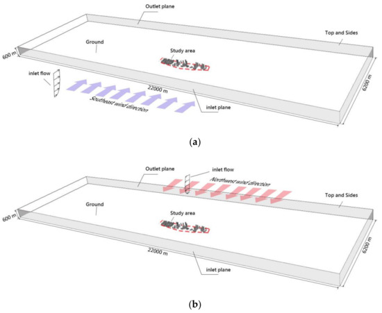
Figure 8.
Computational domain (a) Computational domain in southeast wind; (b) Computational domain in northwest wind.
2.2.5. Grid Discretization
The wind field at pedestrian height was an important content of outdoor wind environment research and adding a ground grid would help to improve the accuracy. Franke et al. [38] propose that the grid between 1.5 m above the ground at the pedestrian speed should not be less than 3 grid units. The height of the measurement point corresponding to the pedestrian height was set as 1.5 m. To improve the calculation accuracy in the study area, the multi-scale grid was used. Therefore, the study area would make the grid size smaller in the study area and larger outside of the area. And the study used the following three kinds of grids: fine grid (minimal grid size was 19 m), middle grid (minimal grid size was 41 m), and coarse grid (minimal grid size was 84 m). The number of x-axis grids was 260 cells, y-axis grids was 148 cells, and z-axis grids was 31 cells. The total was 119,2880 cells (Figure 9).
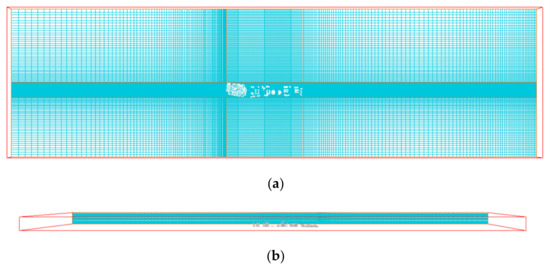
Figure 9.
Grid discretization (a) x-axis and y-axis grid discretization; (b) z-axis grid discretization.
2.2.6. Measuring Points
The wind penetration from different regions will lead to a change in wind environment. For this reason, the change in wind environment was studied in the water area and the street area running through the buildings. According to the skyline model of CFD, 59 measuring points on both north and south sides were selected, which were easily affected by the wind environment. There were 26 measuring points on the north side and 33 measuring points on the south side with frequent activities of people in the area. The specific locations were at the road intersection, the plot entrance of the residential/commercial area, and the building front, as shown in Figure 10.
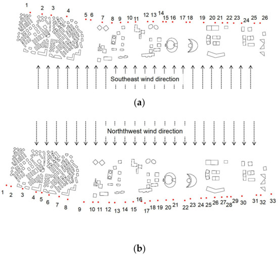
Figure 10.
The measurement points of southeast and northwest wind. (a) The measurement points of southeast wind. (b) The measurement points of northwest wind.
In summary, according to all the conditions (Table 4) were set in Phoenics to simulate outdoor wind environment. From the beginning to the end of the simulation, the run time for both models was 61,402 s, with the total simulation time being 122,804 s. Then the outdoor wind speed distribution at 1.5 m pedestrian height was obtained (Figure 11).
Table 4.
The numerical settings for CFD simulations.
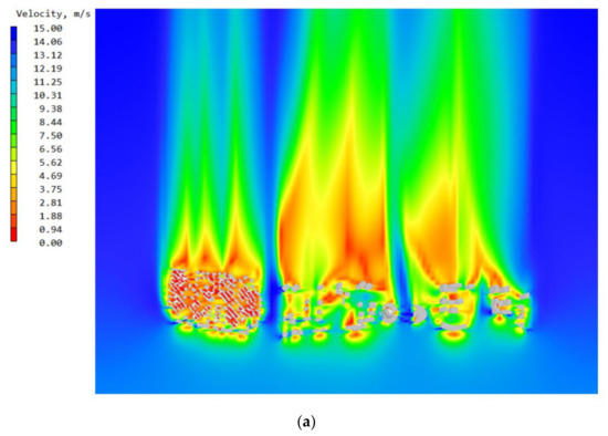
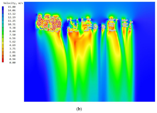
Figure 11.
Southeast and northwest wind simulation (a) Southeast wind simulation, (b) Northwest wind simulation.
2.3. Validation of the CFD Simulation
The reliability of Phoenics was validated by practical measurement in the Qianjiang New City on 1st June 2022. The practical wind direction was selected to be the same as the southeast wind in the study. Then the wind speed data was collected at the site from each measurement point. To obtain the validation results more obviously, the measurement points were divided by plots (Figure 12). And both practical and simulated data of the average wind speed ratio in each plot were calculated by Equation (5) (vr in practice was set as 2.7 m/s according to Hangzhou meteorological data in summer). The practical average wind speed ratio data were compared with Phoenics simulation outputs. It was clear that the average wind speed ratio of each practical measurement point coincided with the corresponding simulated values (Figure 13). The Pearson correlation value R between two data sets was 0.93, and the mean square error was 0.29. This proved the reliability of Phoenics software used in this study.
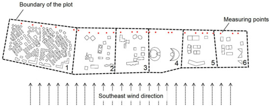
Figure 12.
The subdivision plots with the corresponding measuring points.
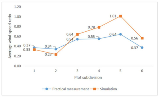
Figure 13.
Average wind speed ratio of practical measurement and simulation results in southeast wind.
3. Results
3.1. Skyline Morphological Characteristics
3.1.1. The Virtual Viewing Field of Hangzhou Qianjiang New City Skyline
The virtual viewing field was calculated according to Equation (9), in which the sight distance D was 1000 m and the height of the viewing field H was calculated at 708 m (Figure 14) [32]. The virtual viewing field was set to 3464 m × 1416 m (Figure 15). The main range of our research was 3464 m × 579 m, which was the main location of the urban construction factors.
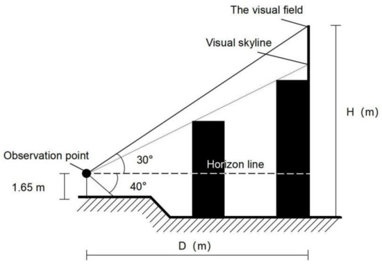
Figure 14.
The field of view for vertical view.
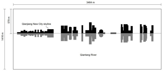
Figure 15.
Hangzhou Qianjiang New City skyline’s virtual view surface.
3.1.2. The Contour Tortuosity of Hangzhou Qianjiang New City Skyline
The skyline contour was drawn according to the skyline model of Hangzhou Qianjiang New City (Figure 16). The skyline was divided into six fluctuations (F) based on the undulation of the skyline. And every fluctuation was formed as a trough-peak-trough. Then, each value of contour tortuosity corresponding to the six fluctuations was calculated according to Equation (1) (Table 5).
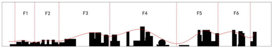
Figure 16.
Hangzhou Qianjiang New City skyline’s contour.
Table 5.
Contour tortuosity data for each wave.
3.1.3. The Building Undulation of Hangzhou Qianjiang New City Skyline
The building undulation of the skyline in Qianjiang New City was calculated in units of a horizontal distance of 100 m (Figure 17). In order to obtain the relationship between building undulation and wind environment, the building undulation was divided into six districts (D) according to the functional regions, and it was calculated in separate districts according to Equation (2) (Table 6).
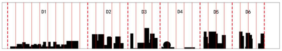
Figure 17.
Hangzhou Qianjiang New City skyline’s building undulation.
Table 6.
Building undulation data for each districts.
3.1.4. The Skyline Rhythm Index of Hangzhou Qianjiang New City Skyline
The skyline rhythm index of the skyline in Qianjiang New City was calculated in the ratio of the fluctuated length of adjacent buildings with a height difference that was more than 30 m to the total skyline length (Figure 18). The skyline rhythm index was divided into six segments (S) according to the functional regions, and it was calculated in separate segments according to Equation (3) (Table 7).
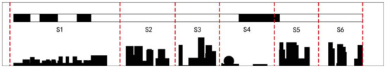
Figure 18.
Hangzhou Qianjiang New City skyline’s skyline rhythm index.
Table 7.
Skyline rhythm index data for each segments.
3.2. Analysis of Wind Environment Results
3.2.1. Data Processing
According to the selection of the location of the measuring points in Figure 10. The measuring points were calculated as the average wind speed ratio and wind speed dispersion for different parts in Equations (5) and (6) (Table 8, Table 9 and Table 10).
Table 8.
Average wind speed ratio and wind speed dispersion at different wind directions for contour tortuosity.
Table 9.
Average wind speed ratio and wind speed dispersion at different wind directions for building undulation.
Table 10.
Average wind speed ratio and wind speed dispersion at different wind directions for skyline rhythm index.
3.2.2. Correlation Test
The study was conducted by using K-S sample analysis in Statistical product and Service Solutions (SPSS) software. The test proved that the significance value P of contour tortuosity, building undulation, skyline rhythm index, with the average wind speed ratio, and wind speed dispersion in different directions, was greater than 0.05. Thus, the data was a normal distribution, and it could perform the Pearson correlation analysis (Table 11).
Table 11.
The significance test.
After the data were normally distributed, the study was conducted by bivariate statistics in SPSS software. Following that, the correlation values R of contour tortuosity, building undulation, and skyline rhythm index with the average wind speed ratio and wind speed dispersion in different wind directions were obtained. The values of R were greater than 0.30, which proved the variables were correlated. It was possible to research the relationship between them (Table 12).
Table 12.
The Pearson correlation.
3.2.3. The Relationship between Wind Environment and Contour Tortuosity
The Relationship between the Average Wind Speed Ratio and Contour Tortuosity
The average wind speed ratio corresponding to 6 fluctuations (F) was integrated with the contour tortuosity (Table 13). The curve fitting was based on the scatter point distribution under southeast and northwest winds (Figure 19). Then the curves between contour tortuosity x and average wind speed ratio y were presented.
Table 13.
The data of the average wind speed ratio and contour tortuosity.
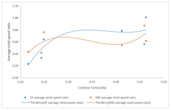
Figure 19.
The relationship between the average wind speed ratio and contour tortuosity.
We defined the curves of the southeast and northwest wind as follows:
Contour tortuosity and average wind speed ratio were positive correlations. This proved that when contour tortuosity increased, the wind permeability would be better. The trends of the curves were both increasing, then decreasing, and increasing again. This indicated that the amplification or attenuation effect of different contour tortuosities on wind speed was consistent in different seasons. In terms of values, the two curves indicated different conditions in summer and winter. The average wind speed was greater in summer than in winter. And the average wind speed ratio changed more significantly in summer than in winter, when the ventilation efficiency was higher.
For the curve inflection points, the presence of two inflection points indicated that when the contour tortuosity exceeded a value, the average wind speed ratio would increase or decrease instead. The average wind speed ratio increased when contour tortuosity was at the two southeast wind inflection points, at 0.34 and 0.42. When the contour tortuosity was 0.34, the average wind speed ratio reached its first large value of 0.8. Then it is followed by an increase in x value and a decrease in y value with a more moderate downward trend. And when x was 0.42, this trend reversed again. The northwest wind had the same trend as the southeast wind, and the values fluctuated to a greater extent. These two inflection points were 0.25 and 0.44, respectively, corresponding to y values of 0.60 and 0.64. In the actual planning to optimize contour tortuosity, the values at the inflection points need to be concerned to balance their wind environment.
While ensuring that the wind speed ratio met the comfort interval (0.50, 2.00), the contour tortuosity x values were in the interval [0.25, 0.59] under the southeast wind and [0.23, 0.55] under the northwest wind. The designer could find the optimal solution for the skyline from within the range.
The Relationship between the Wind Speed Dispersion and Contour Tortuosity
The wind speed dispersion corresponding to 6 fluctuations (F) was integrated with the contour tortuosity (Table 14). The curve fitting was based on the scatter point distribution under southeast and northwest wind (Figure 20). Then the curves between contour tortuosity x and wind speed dispersion y were presented.
Table 14.
The data of the wind speed dispersion and contour tortuosity.
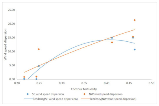
Figure 20.
The relationship between wind speed dispersion and contour tortuosity.
We defined the curves of the southeast and northwest wind as follows:
As can be seen, both curves were parabolic with a downward opening, and the wind speed dispersion in both wind directions showed an increasing and then decreasing trend. Maximum wind speed dispersion existed for both curves. This proved that when the contour tortuosity increased, the wind distribution would be more unstable. It needed to focus on the value of tortuosity corresponding to the maximum value of dispersion.
For the trend of two curves, the wind speed dispersion became larger with increasing contour tortuosity in winter, while the inflection point occurred earlier in summer. This indicated that increasing contour tortuosity caused unstable wind speeds in the winter riverfront area. Designers needed to show special attention to the outdoor wind environment distribution in winter when the contour tortuosity was high. For the values, the maximum values of southeast wind in summer and northwest wind in winter were x = 0.41, y = 14.20 and x = 1.00, y = 31.58, respectively. Within the range of contour tortuosity to satisfy the visual pleasure, when the contour tortuosity was farther from 0.41, the outdoor wind environment would be more steadily distributed in summer. When the contour tortuosity was far from 1.00, the outdoor wind environment would be steadier in winter.
3.2.4. The Relationship between Wind Environment and Building Undulation
The Relationship between the Average Wind Speed Ratio and Building Undulation
The average wind speed ratio corresponding to 6 districts (D) was integrated with the building undulation (Table 15). The curve fitting was based on the scatter point distribution under southeast and northwest winds (Figure 21). Then the curves between building undulation x and average wind speed ratio y were presented.
Table 15.
The data of the average wind speed ratio and building undulation.
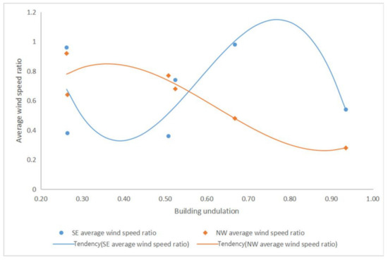
Figure 21.
The relationship between the average wind speed ratio and building undulation.
We defined the curves of the southeast and northwest wind as follows:
For the trend of the curves, the two curves went in the opposite trend. The curve in the southeast wind decreased, then increased and decreased again, while the curve in the northwest wind was the opposite. This proved that the effect of different building undulations on the amplification or attenuation of wind speed in different seasons was the opposite. Meanwhile, the southeast wind curve was steep with a large variation in the average wind speed ratio. The northwest wind curve, in contrast, was relatively flat. Thus, the changes in building undulation had a greater impact on the summer wind environment.
For the curves, when the two curves intersected at x = 0.25, 0.56, and 0.95, the winter to summer average wind speed ratio was equal. The inflection points of the southeast wind curve appeared at x = 0.39 and x = 0.77, corresponding to a minimum point of y = 0.33 and a maximum point of y = 1.15 for the average wind speed ratio. The two inflection points for the northwest wind were x = 0.88 and x = 0.36, corresponding to y values of 0.26 and 0.85.
While the comfort interval requirement of (0.50, 2.00) was ensured to be met, the values of the building undulation x for the two curves were taken to be in the range of [0.13, 0.30] ∪ [0.50, 0.93] for the southeast wind and [0.15, 0.65] ∪ [1.06, 1.30] for the northwest wind.
The Relationship between the Wind Speed Dispersion and Building Undulation
The wind speed dispersion corresponding to 6 districts (D) was integrated with the building undulation (Table 16). The curve fitting was based on the scatter point distribution under southeast and northwest winds (Figure 22). Then the curves between building undulation x and wind speed dispersion y were presented.
Table 16.
The data of the wind speed dispersion and building undulation.
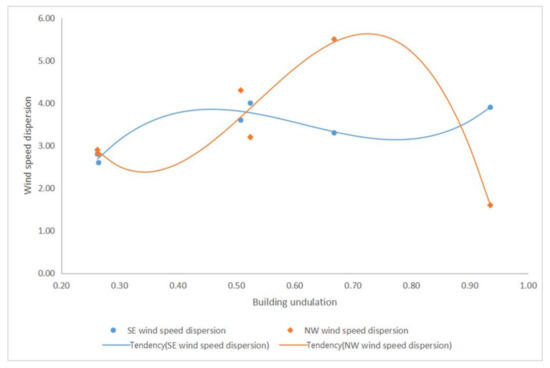
Figure 22.
The relationship between wind speed dispersion and building undulation.
We defined the curves of the southeast and northwest wind as follows:
For the trend of the curves, the two curves were in a complementary state. The southeast wind speed dispersion curve was stable with less fluctuation. And the northwest wind curve was relatively steep and would increase rapidly as the building undulation increased after the minimum value occurred. Especially when the building undulation was greater than 0.72, the wind speed dispersion decreased sharply, and the wind environment tended to be stable. This indicated that the changes in building undulation have a large impact on the uniform distribution of the wind environment in winter, which caused unstable wind speeds in the riverfront area in winter. Therefore, designers needed to pay special attention to the outdoor wind distribution in winter when improving the building’s undulation. The maximum values of southeast wind in summer and northwest wind in winter were x = 0.46, y = 3.85, x = 0.72, y = 5.62, and the minimum values were x = 0.77, y = 3.13, x = 0.34, y = 2.38, respectively.
3.2.5. The Relationship between Wind Environment and Skyline Rhythm Index
The Relationship between the Average Wind Speed Ratio and Skyline Rhythm Index
The average wind speed ratio corresponding to six segments (S) was integrated with the skyline rhythm index (Table 17). The curve fitting was based on the scatter point distribution under southeast and northwest winds (Figure 23). Then the curves between skyline rhythm index x and average wind speed ratio y were presented.
Table 17.
The data of the average wind speed ratio and skyline rhythm index.
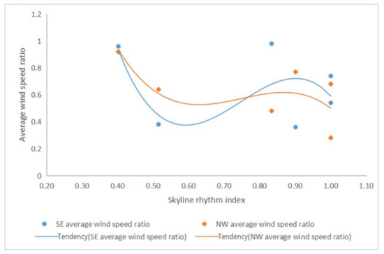
Figure 23.
The relationship between the average wind speed ratio and skyline rhythm index.
We defined the curves of the southeast and northwest wind as follows:
For the trend of the curves, both curves have a negative correlation in trend. When the skyline rhythm index increased, the curves of the average wind speed ratio both decreased, then increased and decreased again. This meant that the effect of different skyline rhythm indexes on the amplification or attenuation of wind speed was similar for different seasons. It was found that the changes in the wind speed ratio in the summer wind environment were more sensitive to the numerical changes, and the curve fluctuations were much more intense in the curves of the relationship between the three quantitative factors and the average wind speed ratio. For the curve inflection points, two inflection points indicated that when the skyline rhythm index exceeded a value, the average wind speed ratio increased or decreased conversely. The y value gradually decreased to 0.38 during the southeast wind curve index from 0 to 0.59. And the x value gradually increased to 0.90 and the average wind speed ratio increased to 0.72. Subsequently, the y decreased as x increased. The northwest wind had the same trend as the southeast wind, and the two inflection points were x = 0.63 and x = 0.87, respectively, corresponding to y values were 0.53 and 0.62.
To ensure that the two curves were in the range of (0.5, 2), the values of the skyline rhythm index x were taken in the range of [0.29, 0.49] ∪ [0.72, 1.03] for the southeast wind and [0.24, 1] for the northwest wind, respectively.
The Relationship between the Wind Speed Dispersion and Skyline Rhythm Index
The wind speed dispersion corresponding to six segments (S) was integrated with the skyline rhythm index (Table 18). The curve fitting was based on the scatter point distribution under southeast and northwest winds (Figure 24). Then the curves between skyline rhythm index x and wind speed dispersion y were presented.
Table 18.
The data of the wind speed dispersion and skyline rhythm index.
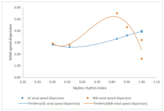
Figure 24.
The relationship between wind speed dispersion and skyline rhythm index.
We defined the curves of the southeast and northwest wind as follows:
For the trend of the curves, the two curves showed different trends. The skyline rhythm index of the southeast wind curve becomes larger as the dispersion shows an overall increasing trend. And the curve was relatively stable. The northwest wind curve was more variable. After the minimum value of wind speed dispersion appeared, it increased sharply to 5.23. Then it decreased to a maximum value of wind speed dispersion at x = 0.81. We found that the changes in the wind environment in winter were more sensitive to the numerical changes, and the curves mostly showed intense fluctuation. When x was less than 0.81, the wind environment would be steadily distributed. This meant that the skyline rhythm index should be far from 0.81 to ensure a stable distribution of the wind environment.
In summary, the equation of the skyline quantitative factors with the average wind speed ratio/wind speed dispersion and their comfort judgment were shown in the following Table 19 and Table 20.
Table 19.
The relationships between skyline quantification factors and average wind speed ratio.
Table 20.
The relationships between skyline quantification factors and wind speed dispersion.
4. Discussion
This paper is to discover the distribution pattern of the wind environment in the skyline area. To our knowledge, it is the first study in the literature to reveal the relationship between the skyline quantitative factors and the outdoor wind environment, which is our major contribution to the literature. Nonetheless, there are several issues deserving further discussion.
Skyline morphological changes bring different aesthetic perceptions. Visual perception is the dominant sensory perception in the European Landscape Convention (ELC), accounting for 87% of all senses [39]. And it is the first way for people to perceive the urban style. Zhu [40] proposed that the aesthetic experience of the city skyline depends on the interweaving of material and perceptual. People can get visual feelings and aesthetic perception from the changing morphology of the skyline. Thus, it is essential to discuss how to control the skyline morphology in urban design so that it can bring visual aesthetics.
The city skyline is composed of natural and urban construction factors, which will affect the microclimate. It is crucial for the skyline to create a comfortable microclimate while ensuring its aesthetics. The wind environment is one of the important factors affecting the urban microclimate. Nevertheless, the current stage of skyline designs often ignores the significance of the outdoor wind environment. Hence, the balance between aesthetics and microclimate should be considered in the process of urban construction. It is important to discuss the range to ensure the aesthetics of the city skyline while guaranteeing the comfort of the outdoor wind environment.
However, there are still some limitations to this paper. First, the skyline contour formed by the combination and variation of building groups in the city is strongly correlated with aesthetic perception. It should be mentioned that the paper only researched the following three factors of the skyline contour: contour tortuosity, building undulation, and skyline rhythm index. It lacked the analysis of other skyline quantitative factors such as hierarchy, roof turnings, and other complex elements.
Second, in order to make the results more intuitive, we ignored the influence of buildings outside the area and focused only on the wind environment changes within the study area. Moreover, the relationship between the wind environment and quantitative factors in this paper took Hangzhou as an example. And we only analyzed the weather conditions in Hangzhou, which led to a weak generalization of the relational equation. Later studies should select more cities for wind environment simulation in order to obtain optimization strategies with a wider range of applications.
Third, this paper explored the relationship between correlated factors (R > 0.3). However, it does not distinguish between strong (R > 0.5) and weak (0.5 > R > 0.3) correlations. The next step would be explored in depth when more factors are introduced, depending on the different levels of correlation.
Fourth, the paper was mainly a study on the skyline of Qianjiang New City in Hangzhou, hence the Equations (10)–(21) could only be used in Hangzhou and could not be applied to other cities. In subsequent studies, more cities should be selected for comprehensive consideration to obtain more universal equations with corresponding comfort ranges that can be applied to all cities.
5. Conclusions
In this study, the coupling relationship is proposed to balance visual pleasure and physical comfort intuitively. The study was conducted in Hangzhou, China. The results suggested that there were equations between the skyline quantization factors (contour tortuosity, building undulation, and skyline rhythm index) and the wind environment. The correlation of the factors were individual differences, as follows: a positive correlation between contour tortuosity and wind environment; a negative correlation between building undulation and wind environment. The skyline rhythm index was relatively special, as follows: a negative correlation in the average wind speed ratio and a positive correlation in wind speed dispersion. Meanwhile, the wind environmental curves had inflection points. It should be noted that the increase in quantization factors could cause the wind environment to deteriorate in practical optimization.
For the evaluation method of wind environment, as for the average wind speed ratio, the equations ensured that when the factors were within the appropriate range, the wind speed was guaranteed to be comfortable. As for the wind speed dispersion, it was used as an auxiliary criterion to ensure visual pleasure while judging the wind speed uniformity under different values of factors.
We also found that the changes in the contour tortuosity, building undulation, and skyline rhythm index affected the wind environment with seasonal differences. The average wind speed ratio in summer and the wind speed dispersion in winter were more sensitive to the factor value change. In practical applications, designers should pay particular attention to the changes in ventilation capacity in summer and continuous physical comfort in winter. Our results can provide decision support for the relevant designs on sustainable urban design and deepen the understanding of the living environment from a people-centric perspective.
Author Contributions
Data curation, Z.L., X.Q., J.C., L.S. and X.H.; Methodology, X.Y.; Writing–original draft, J.G. All authors have read and agreed to the published version of the manuscript.
Funding
This research was funded by National Natural Science Foundation of China grant number 51878608, and also funded by Zhejiang Provincial Natural Science Foundation grant number LY22E08004.
Institutional Review Board Statement
Not applicable.
Informed Consent Statement
Not applicable.
Data Availability Statement
Not applicable.
Conflicts of Interest
The authors declare no conflict of interest.
Abbreviations
| CFD | Computational fluid dynamics | ||
| CBD | Central business districts | ||
| SPSS | Statistical product and Service Solutions | ||
| SE | Southeast | ||
| NW | Northwest | ||
| F | Fluctuations | ||
| D | Districts | ||
| S | Segments | ||
| ELC | European Landscape Convention | ||
| KC | Contour tortuosity | ||
| kn | Single band of contour tortuosity | ||
| △H | The sum of differences of each band between the low and high points | meter/meters | m |
| △L | The horizontal distance of each band | meter/meters | m |
| U | building undulation | ||
| △hn | The degree of unit building undulation | meter/meters | m |
| n | The units of building undulation | ||
| Rf | Skyline rhythm index | ||
| w | The length of fluctuation contour | meter/meters | m |
| L | The whole length of the skyline | meter/meters | m |
| Rw | Wind speed ratio | ||
| Vs | The absolute value of wind speed at the measuring point at the pedestrian height | meters per second | m/s |
| v | the absolute value of initial wind speed at The pedestrian height | meters per second | m/s |
| RM | The average wind speed ratio index | ||
| Vi | The absolute value of average wind speed at pedestrian height | meters per second | m/s |
| vr | The absolute value of initial wind speed at the same height | meters per second | m/s |
| σ | Wind speed ratio dispersion | ||
| n | The number of data | ||
| μ | The average of all values | meters per second | m/s |
| L | The width of the visual viewing field | meter/meters | m |
| D | The visual viewing range | meter/meters | m |
| H | The height of viewing field | meter/meters | m |
| U(z) | The average wind speed at height | meters per second | m/s |
| Z | Height | meter/meters | m |
| UG | The average wind speed at the standard height ZG | meters per second | m/s |
| ZG | The standard height | meter/meters | m |
| α | a parameter to describe the surface roughness | ||
| P | The significance value | ||
| R | The correlation values | ||
References
- Fisher-Gewirtzman, D.; Burt, M.; Tzamir, Y. A 3-d visual method for comparative evaluation of dense built-up environments. Environ. Plan. B Plan. Des. 2003, 30, 575–587. [Google Scholar] [CrossRef]
- Zhang, J.; Pan, L. Arrangement and creation of urban horizon landscape in coastal city around mountains—Case study on the coastal skyline of Yantai City. Urban Stud. 2010, 17, 77–84. [Google Scholar]
- Niu, X.; Li, K. A quantitative to visual impact analysis of city skyline. Urban Plan. Forum 2013, 3, 99–105. [Google Scholar]
- Shi, Y.; Cao, J.; Zhu, X. City skyline aesthetic analysis based on evaluation model. Mod. Urban Res. 2018, 10, 67–74. [Google Scholar]
- Stamps, A.; Nasar, J.L.; Hanyu, K. Using pre-construction validation to regulate urban skylines. J. Am. Plan. Assoc. 2005, 71, 73–91. [Google Scholar] [CrossRef]
- Imamoglu, Ç. Complexity, liking and familiarity: Architecture and non-architecture Turkish students’ assessments of traditional and modern house facades. J. Environ. Psychol. 2000, 20, 5–16. [Google Scholar] [CrossRef]
- Stamps, A. Fractals, skylines, nature and beauty. Landsc. Urban Plan. 2002, 60, 163–184. [Google Scholar] [CrossRef]
- Nasar, J.; Terzano, K. The desirability of views of city skylines after dark. J. Environ. Psychol. 2010, 30, 215–225. [Google Scholar] [CrossRef]
- Le, D.; Li, N.; Su, L.; .Li, J.; Wei, X. Numerical simulation of wind environment in the urban areas. Saf. Environ. 2012, 12, 257–262. [Google Scholar]
- Zhou, X.; Chen, H. A research on the impact of different city development models on climates in central urban areas: A case study of Wuhan. Archit. Pract. 2019, 2, 27–28. [Google Scholar]
- Zhao, Q.; Zhang, T. A preliminary study on the integration of evaluation methods and strategies for urban outdoor wind environment. In Proceedings of the 2015 China Urban Planning Annual Conference, Guiyang, China, 19–21 September 2015; pp. 215–229. [Google Scholar]
- Van Hove, L.W.A.; Jacobs, C.M.J.; Heusinkveld, B.G.; Elbers, J.A.; van Driel, B.L.; Holtslag, A.A.M. Temporal and spatial variability of urban heat island and thermal comfort within the Rotterdam agglomeration. Build. Environ. 2015, 83, 91–103. [Google Scholar] [CrossRef]
- Adamek, K.; Vasan, N.; Elshaer, A.; English, E.; Bitsuamlak, G. Pedestrian level wind assessment through city development: A study of the financial district in Toronto. Sustain. Cities Soc. 2017, 35, 178–190. [Google Scholar] [CrossRef]
- Zhuang, A.; Gao, C.; Ling, Z. Numerical simulation of the wind field around different building arrangements. Wind Eng. Ind. Aerodyn. 2005, 93, 891–904. [Google Scholar] [CrossRef]
- Chen, H. The effect of building shape and its arrangement on ventilation efficiency in urban area. J. Wuhan Univ. Technol. 2002, 7, 44–46. [Google Scholar]
- Blocken, B.; Persoon, J. Pedestrian wind comfort around a large football stadium in an urban environment: CFD simulation validation and application of the new Dutch wind nuisance standard. Wind Eng. Ind. Aerodyn. 2008, 96, 621–639. [Google Scholar] [CrossRef]
- Ying, X.; Wang, Y.; Li, W.; Liu, Z.; Ding, G. Group layout pattern and outdoor wind environment of enclosed office buildings in Hangzhou. Energies 2020, 13, 406. [Google Scholar] [CrossRef]
- Takebayashi, H.; Moriyama, M.; Miyake, K. Analysis on the relationship between properties of urban block and wind path in the street canyon for the use of the wind as the climate resources. J. Environ. Eng. 2009, 74, 77–82. [Google Scholar] [CrossRef][Green Version]
- Shan, Y.; Cai, X.; Zhang, D. Research on comfortable spatial pattern of microclimate in waterfront residential areas of cold regions: A case study of Tianjiahu Residential Area in Tianjin. Build. Sci. 2022, 38, 82–88. [Google Scholar]
- Zhang, H.; Yang, W. The application of natural ventilation in the traditional dwelling. Archit. Cult. 2016, 2, 164–165. [Google Scholar]
- Chang, C.-H.; Meroney, R.N. Concentration and flow distributions in urban street canyons: Wind tunnel and computational data. J. Wind Eng. Ind. Aerodyn. 2003, 91, 1141–1154. [Google Scholar] [CrossRef]
- Ma, J.; Chen, S. Numerical study of plan arrangement effect on wind environment around tall buildings. J. Zhejiang Univ. 2007, 9, 1477–1481. [Google Scholar]
- Blocken, B.; Carmeliet, J. Guidelines for the required time resolution of meteorological input data for wind-driven rain calculations on buildings. J. Wind Eng. Ind. Aerodyn. 2008, 96, 621–639. [Google Scholar] [CrossRef]
- Chen, L.; Hang, J.; Sandberg, M.; Claesson, L.; Di Sabatino, S.; Wigo, H. The impacts of building height variations and building packing densities on flow adjustment and city breathability in idealized urban models. Build. Environ. 2017, 118, 344–361. [Google Scholar] [CrossRef]
- Jian, H.; Yu, G. Ventilation strategy and air change rates in idealized high-rise compact urban areas. Build. Environ. 2010, 45, 2754–2767. [Google Scholar]
- Kono, T.; Tamura, T.; Ashie, Y. Numerical investigations of mean winds within canopies of regularly arrayed cubical buildings under neutral stability conditions. Bound. Layer Meteorol. 2009, 134, 131–155. [Google Scholar] [CrossRef]
- Yang, J.; Pan, Y.; Shi, B. Evaluation of overlooking views of city central district:the case of Hong Kong. Urban Plan. Forum 2013, 5, 106–112. [Google Scholar]
- Lyu, S.; Yan, T.; Li, L. Comparison of the studies on quantitative index evaluation of urban skyline aesthetics. Hous. Sci. 2019, 39, 27–31. [Google Scholar]
- Kubota, T.; Miura, M.; Tominaga, Y.; Mochida, A. Wind tunnel tests on the relationship between building density and pedestrian-level wind velocity: Development of guidelines for realizing acceptable wind environment in residential neighborhoods. Build. Environ. 2008, 43, 1699–1708. [Google Scholar] [CrossRef]
- Xie, Z.; Lu, Y.; Yu, X. Experimental investigation on pedestrian-level wind environment around a high-rise building. J. Tongji Univ. 2020, 48, 1726–1732. [Google Scholar]
- Ye, Z. Wind environment oriented urban block spatial design-a case study of CAUP area Tongji University. In Proceedings of the 2010 Urban Development and Planning International Conference, Qinhuangdao, China, 22 June 2010; pp. 301–305. [Google Scholar]
- Niu, X.; Xu, F. Quantitative evaluation of spatial openness of built environment using visual impact analysis. Urban Plan. Forum 2011, 1, 91–97. [Google Scholar]
- Zhuang, Z.; Yu, Y.; Ye, H.; Tan, H.; Xie, J. Review on CFD simulation technology of wind environment around buildings. Build. Sci. 2014, 30, 108–114. [Google Scholar]
- Franke, J.; Hellsten, A.; Schlunzen, K.; Carissimo, B. The COST 732 Best Practice Guideline for CFD simulation of flows in the urban environment: A summary. Int. J. Environ. Pollut. 2011, 44, 419. [Google Scholar] [CrossRef]
- Yu, B.; He, X.; Wei, L.; Chen, L.; Zhou, W. Primary exploration for construction of urban multilevel ventilation corridors system in Hangzhou. J. Meteorol. Sci. 2018, 38, 625–636. [Google Scholar]
- Davenport, A.G. An approach to human comfort criteria for environment wind conditions. In Proceedings of the the Colloquium on Building Climatology, Stockholm, Sweden, 4–6 September 1972. [Google Scholar]
- Yoshie, R.; Mochida, A.; Tominaga, Y.; Kataoka, H.; Harimoto, K.; Nozu, T.; Shirasawa, T. Cooperative project for CFD prediction of pedestrian wind environment in the Architectural Institute of Japan. J. Wind Eng. Ind. Aerodyn. 2007, 95, 1551–1578. [Google Scholar] [CrossRef]
- Franke, J.; Hirsch, C.; Jensen, A.G.; Krüs, H.W.; Schatzmann, M.; Westbury, P.S.; Miles, S.D.; Wisse, J.A.; Wright, N.G. Recommendations on the use of CFD in wind engineering. In COST Action C14, Impact of Windand Storm on City Life Built Environment, Proceedings of the International Conference on Urban Wind Engineeringand Building Aerodynamics, Rhode-St-Genèse, Belgium, 5–7 May 2004; Van Beeck, J.P.A.J., Ed.; von Karman Institute: Sint-Genesius-Rode, Belgium, 2004. [Google Scholar]
- Jones, M.; Stenseke, M. The European Landscape Convention; Springer: Dordrecht, The Netherlands, 2011. [Google Scholar]
- Zhu, B. Skyline aesthetics. Urban Plan. Overseas 1987, 03, 35–43. [Google Scholar]
Publisher’s Note: MDPI stays neutral with regard to jurisdictional claims in published maps and institutional affiliations. |
© 2022 by the authors. Licensee MDPI, Basel, Switzerland. This article is an open access article distributed under the terms and conditions of the Creative Commons Attribution (CC BY) license (https://creativecommons.org/licenses/by/4.0/).