
Some Issues in the Seismic Assessment of Shear-Wall Buildings through Code-Compliant Dynamic Analyses

 ,
,  ,
, 
Abstract
:1. Introduction
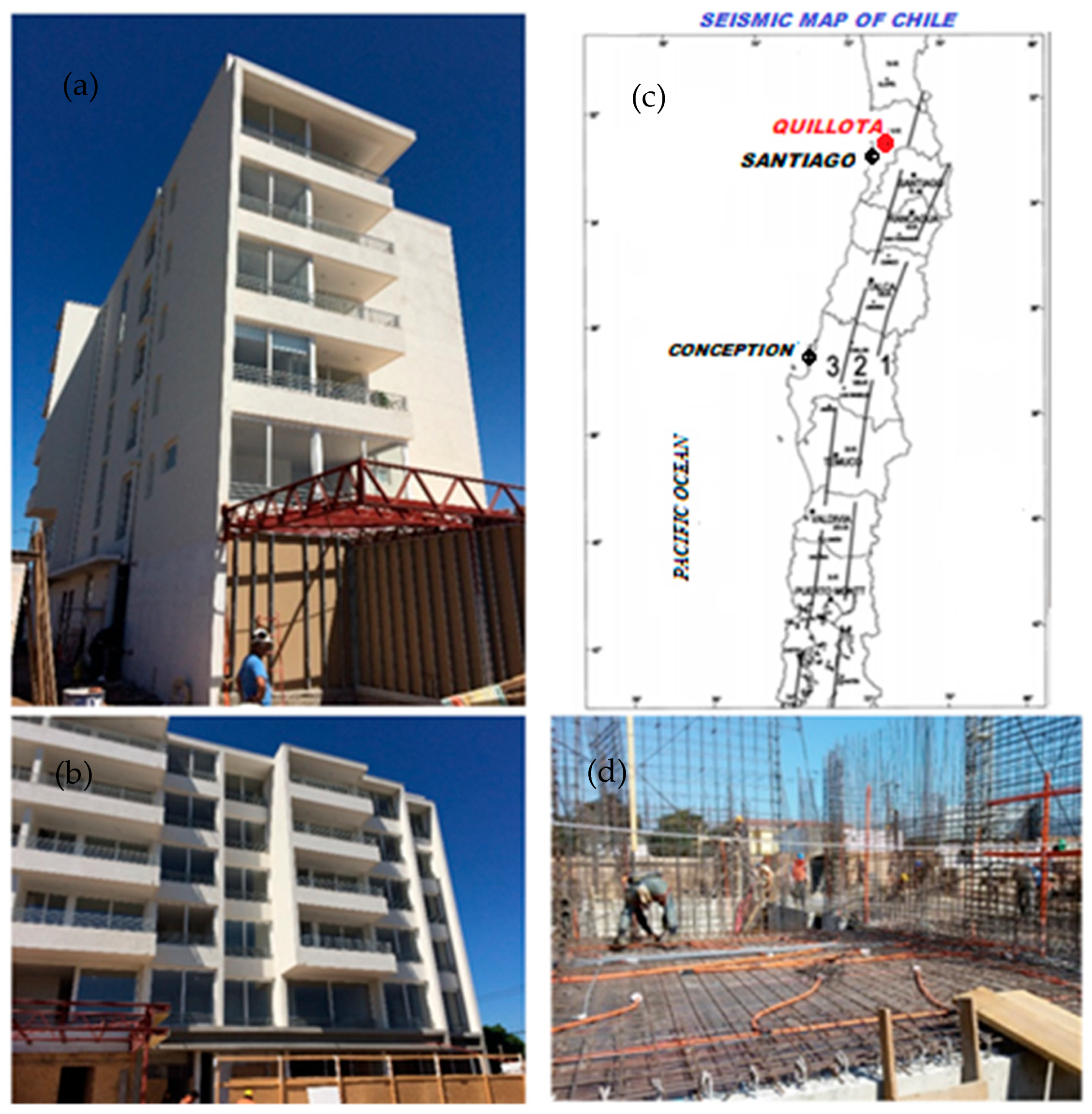
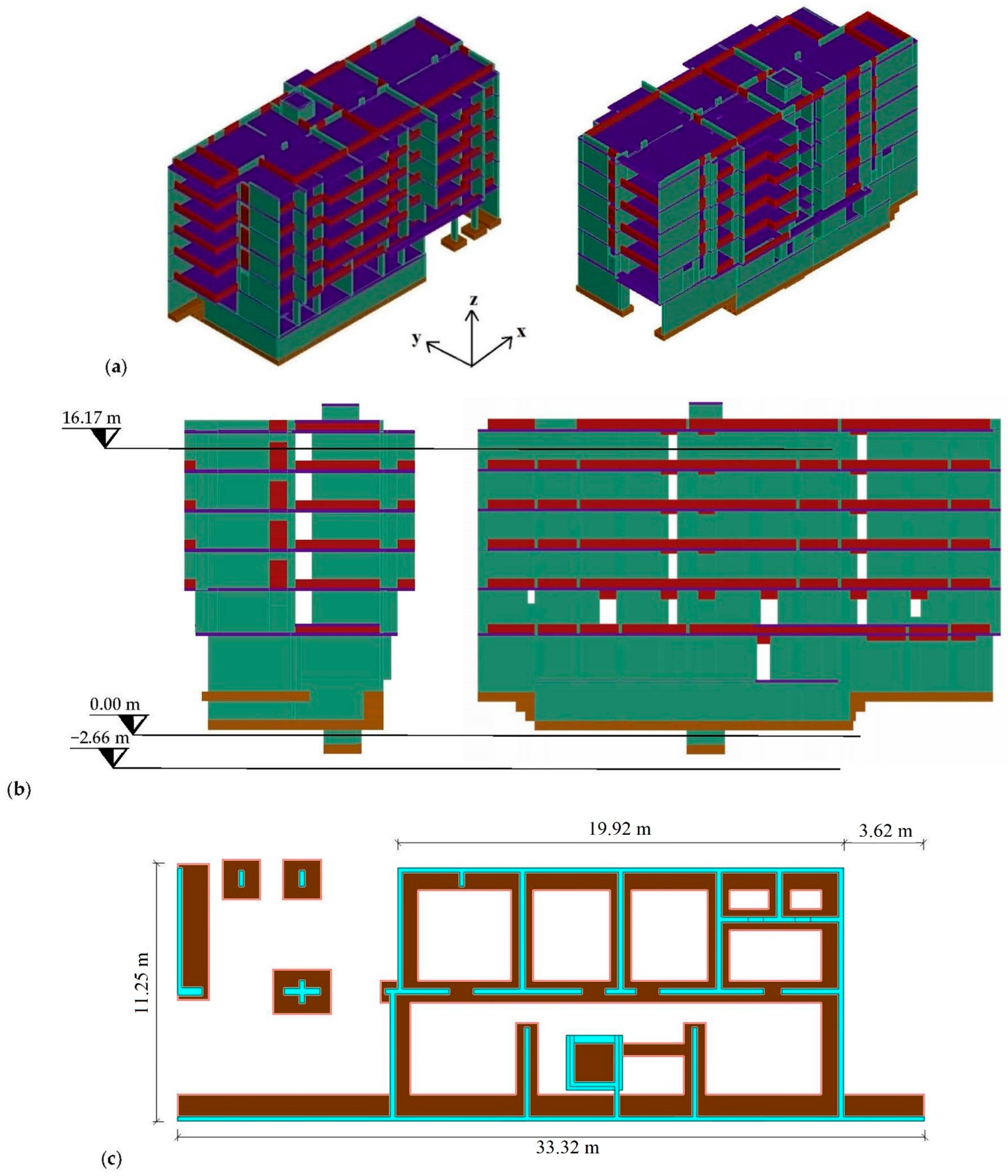
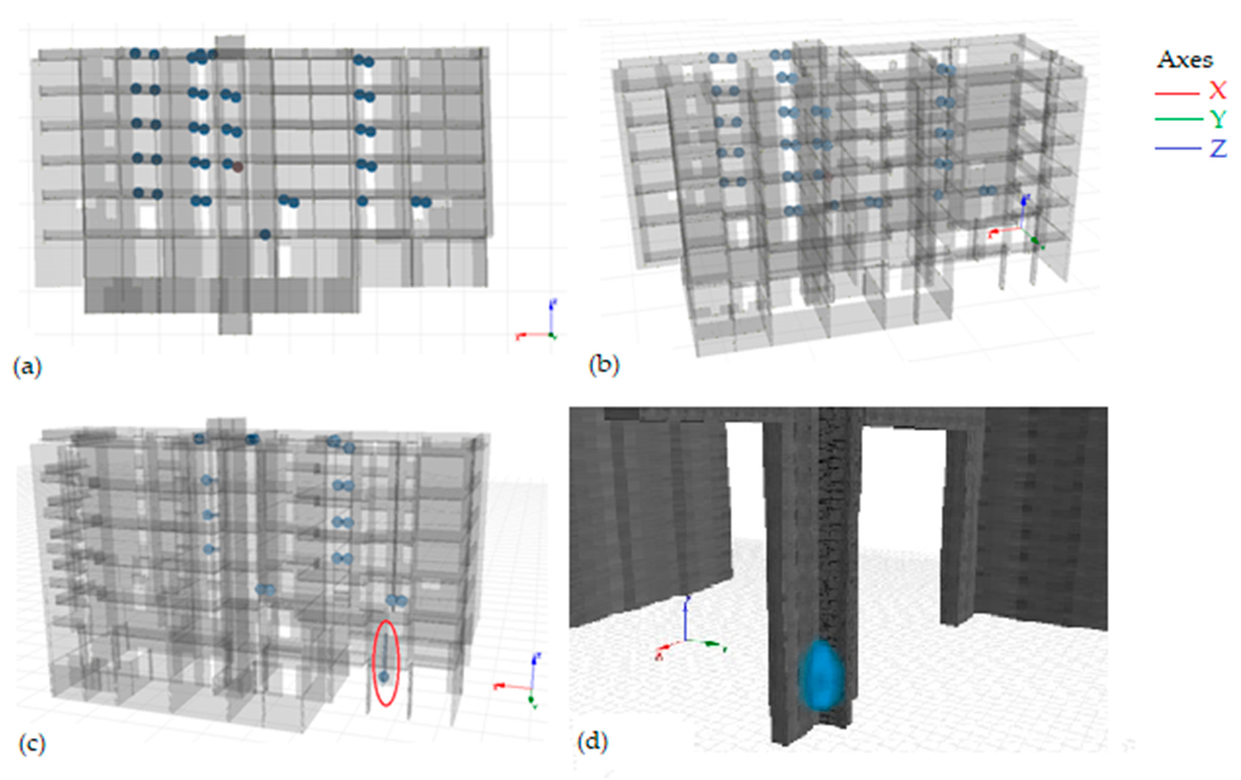
2. Case-Study RC-SW Building
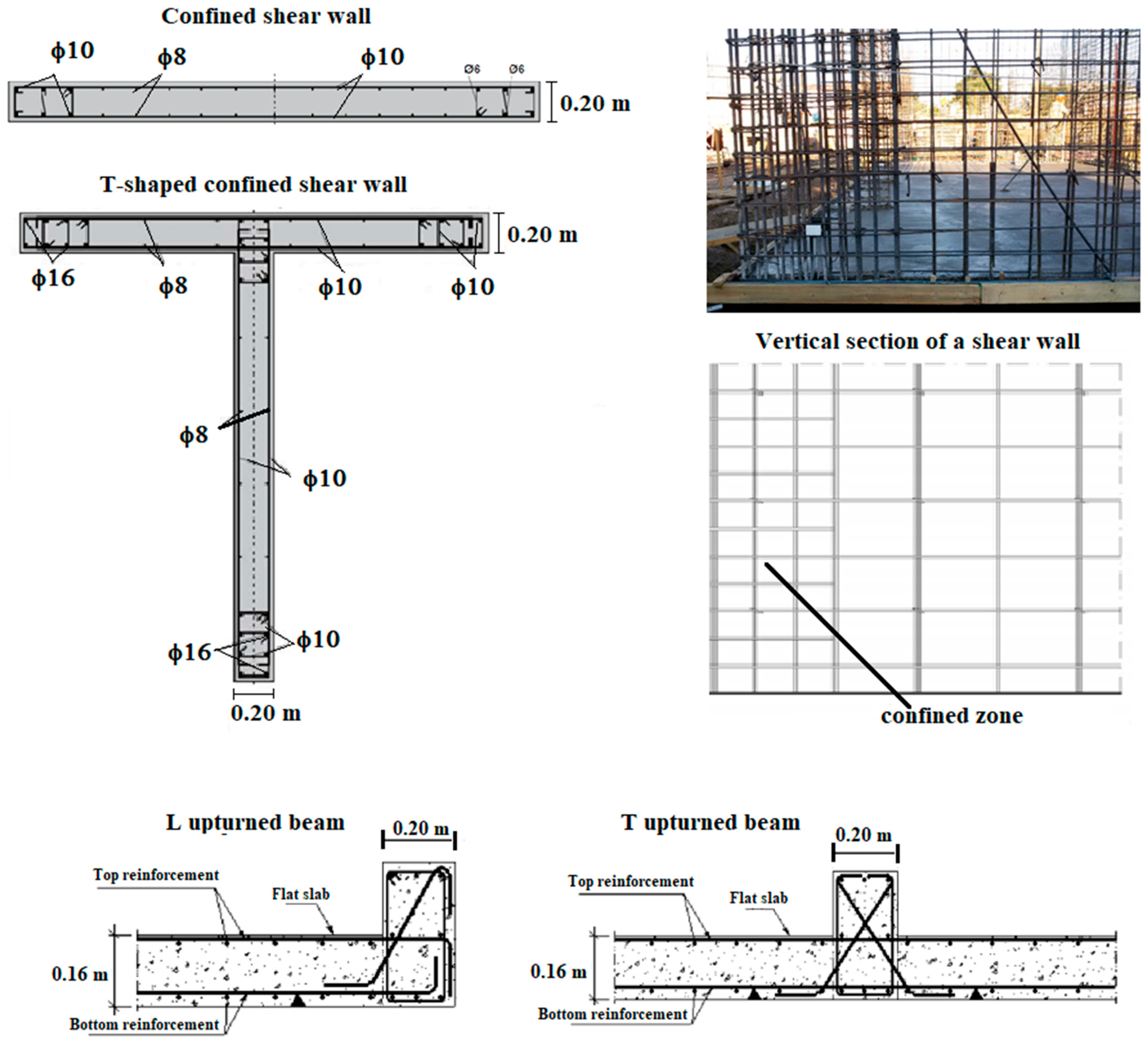
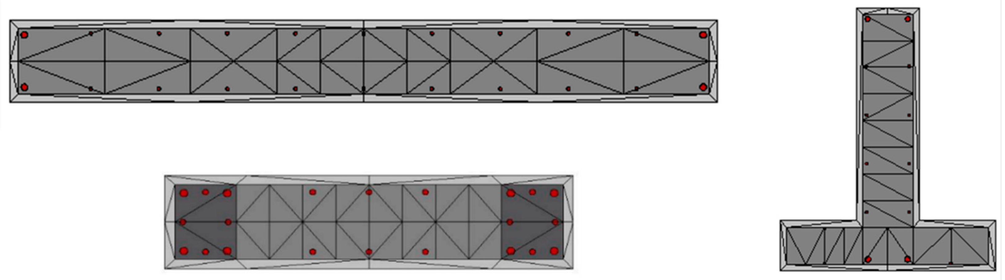
Numerical Model
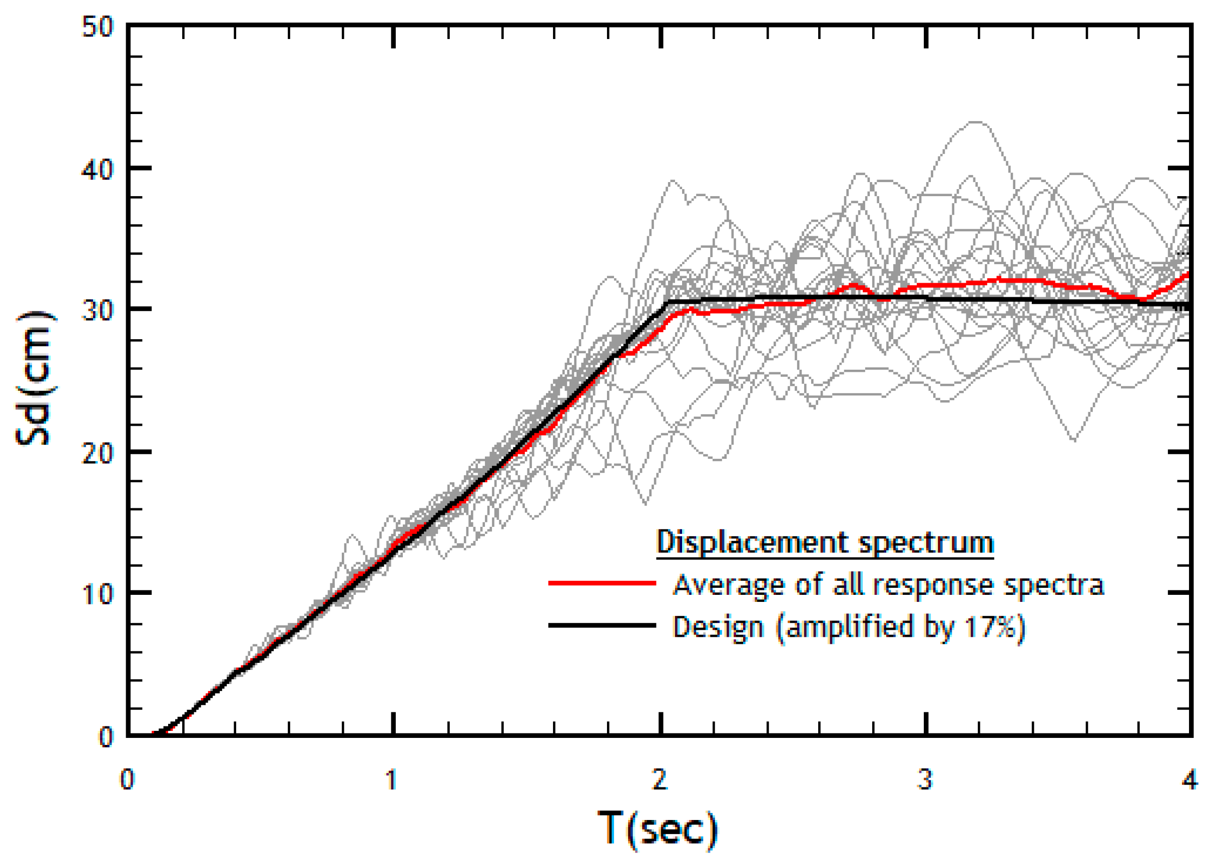
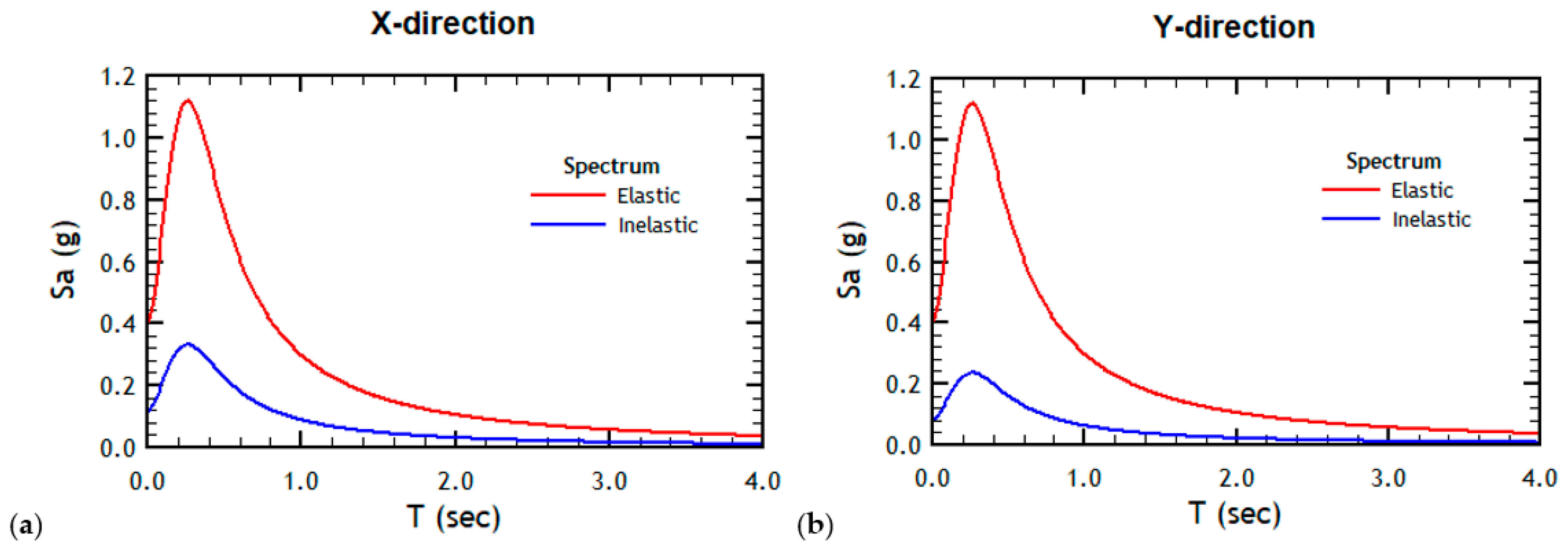
3. Design Response Spectra and Spectrum-Consistent Earthquakes
4. Dynamic Linear Analyses
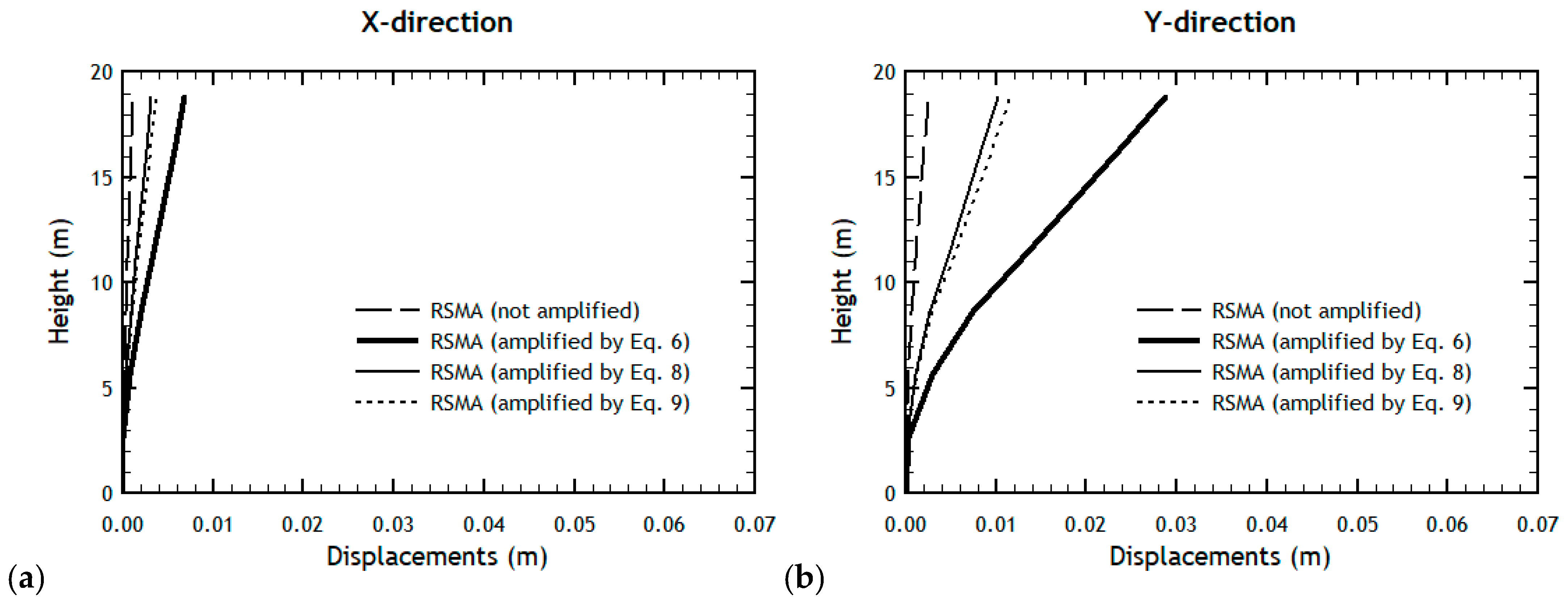
4.1. Modal Response Spectrum Analysis (MRSA)
4.2. Linear Time-History Analysis (LTHA)
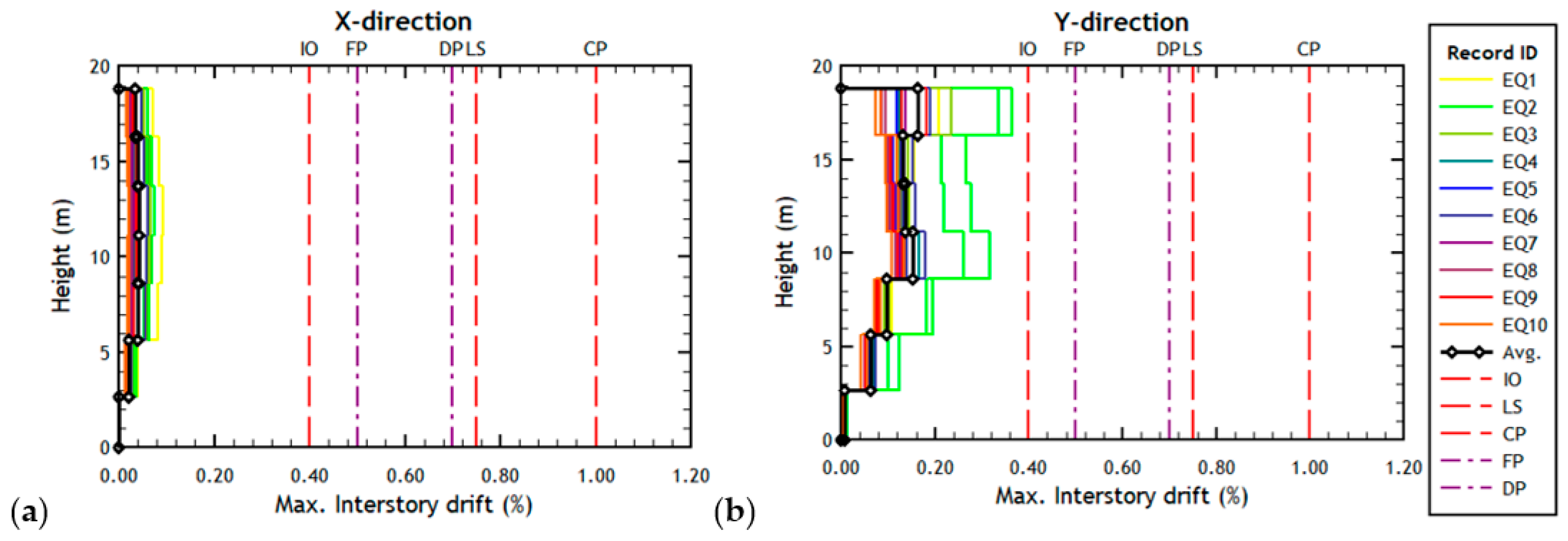
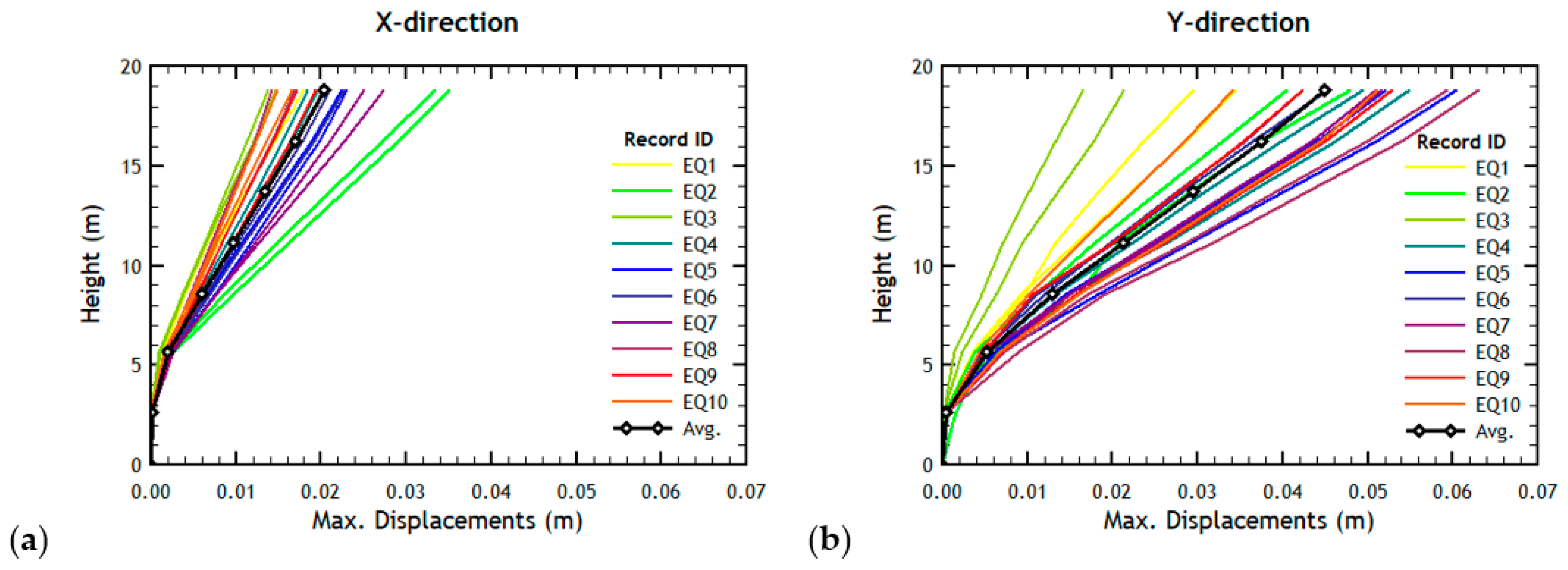
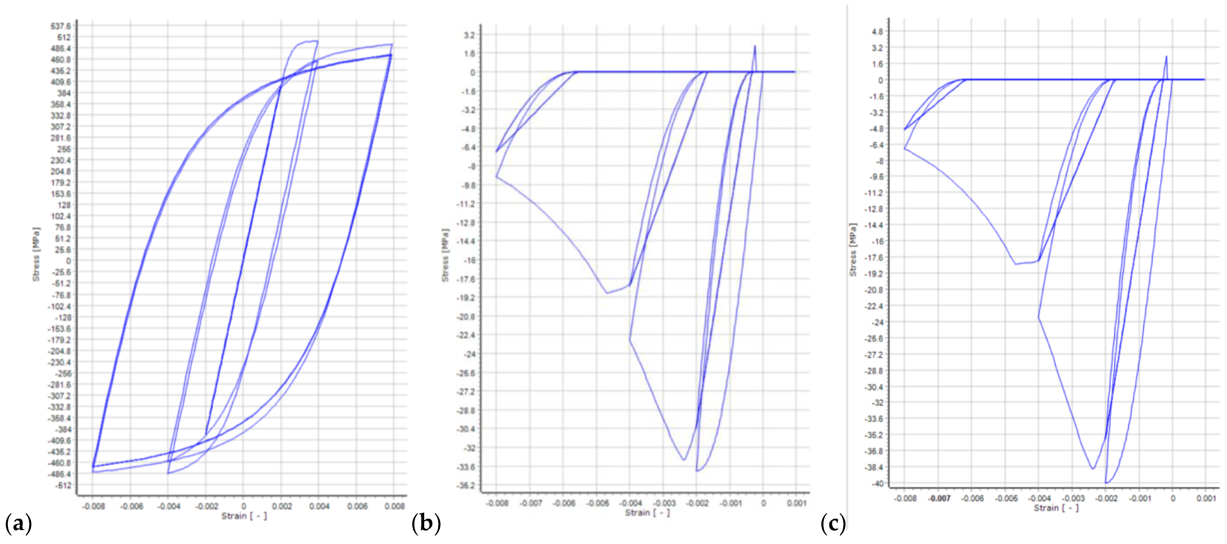
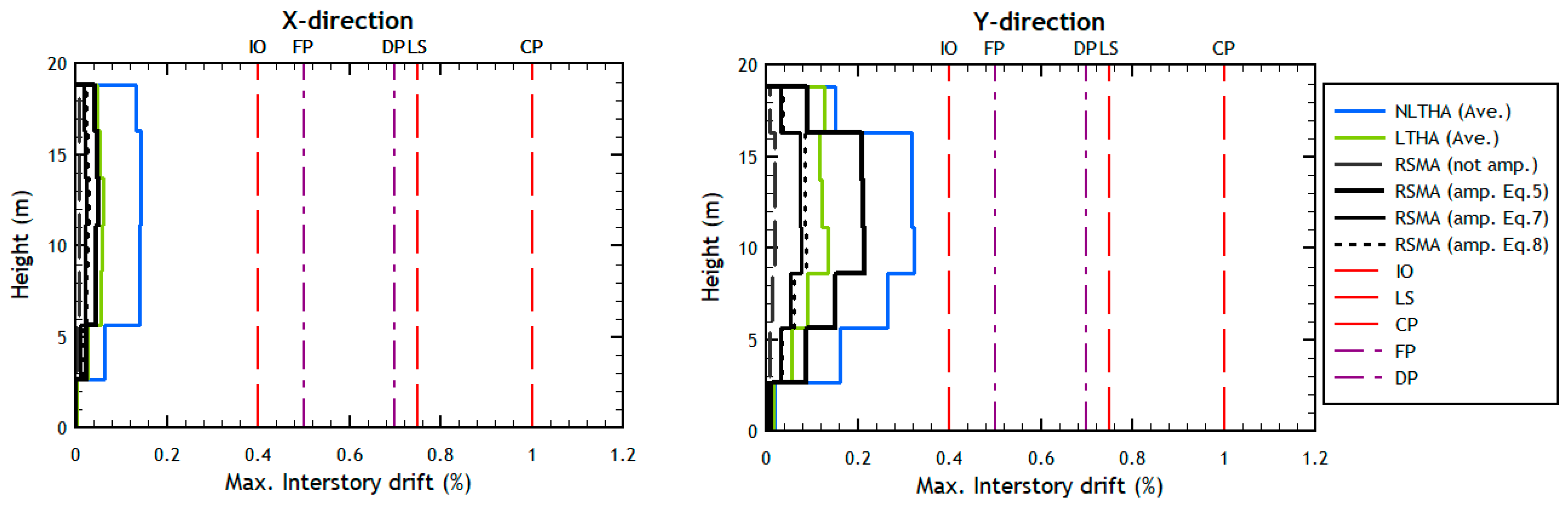
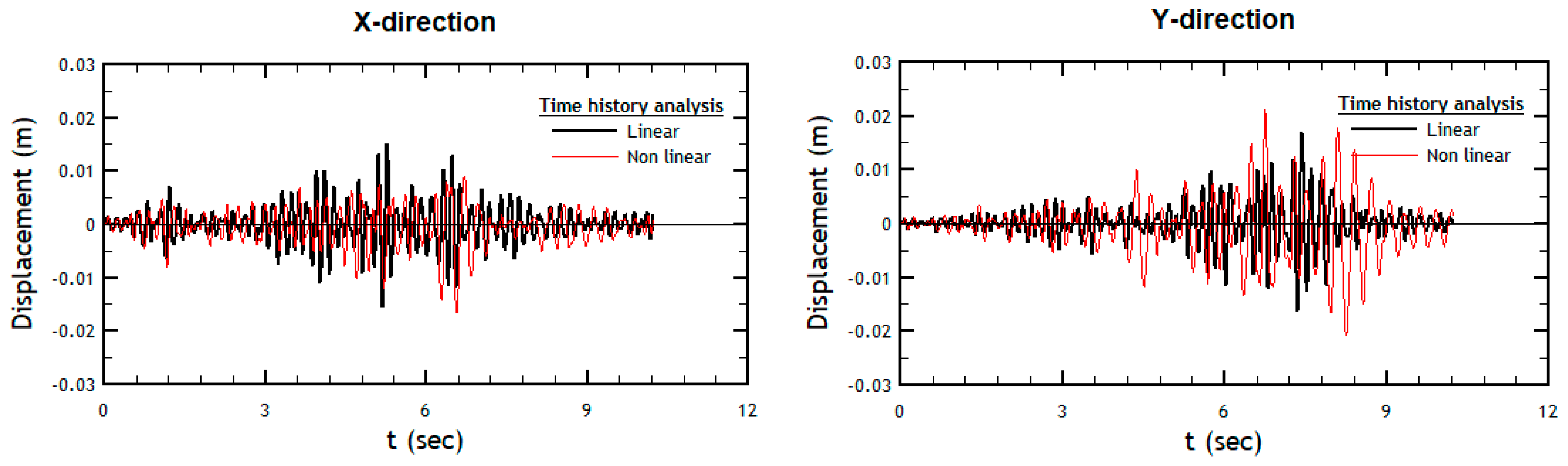
5. Results of the Non-Linear Time-History Analysis (NLTHA)
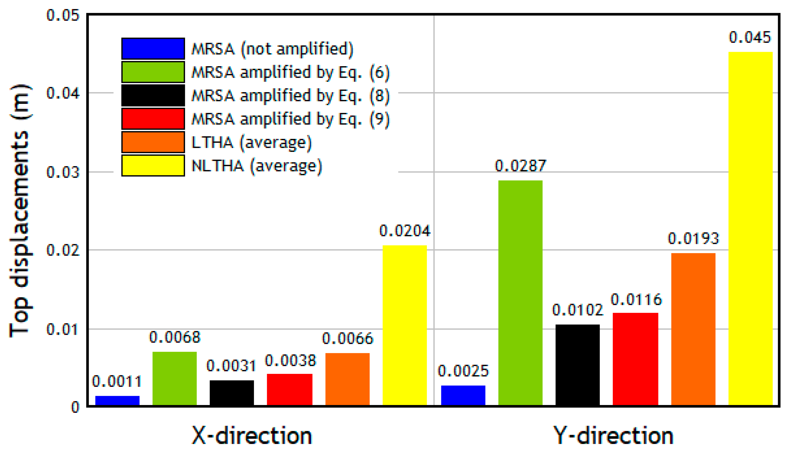
6. Comparing the Results from Linear and Non-Linear Analyses
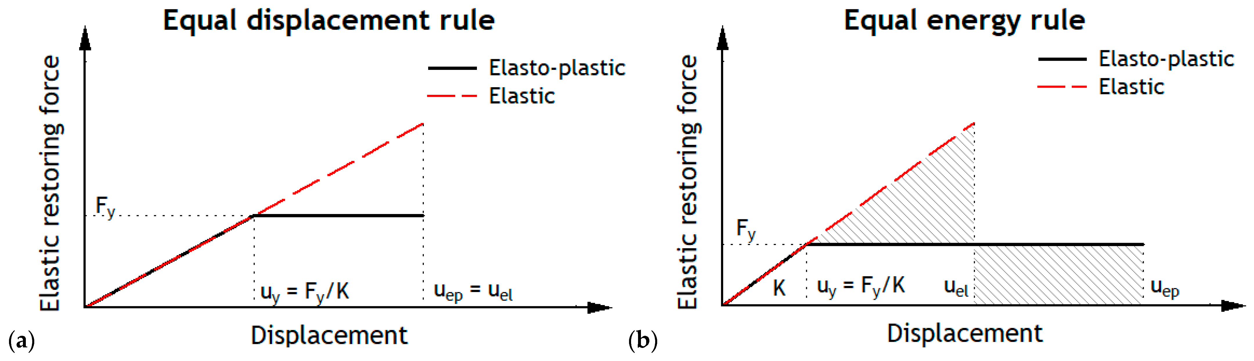
7. Post-Elastic Behavior
8. Concluding Remarks
Author Contributions
Funding
Data Availability Statement
Acknowledgments
Conflicts of Interest
References
- Fintel, M. Performance of buildings with shear walls in earthquakes of the last thirty years. PCI J. 1995, 40, 62–80. [Google Scholar] [CrossRef]
- Ugalde, D.; Lopez-Garcia, D. Behavior of reinforced concrete shear wall buildings subjected to large earthquakes. Procedia Eng. 2017, 199, 3582–3587. [Google Scholar] [CrossRef]
- Ugalde, D.; Lopez-Garcia, D. Analysis of the seismic capacity of Chilean residential RC shear wall buildings. J. Build. Eng. 2020, 31, 101369. [Google Scholar] [CrossRef]
- European Committee for Standardization (CEN). EN 1998-3: Eurocode 8: Design of Structures for Earthquake Resistance; CEN: Brussels, Belgium, 2004. [Google Scholar]
- ASCE/SEI 7-16; Minimum Design Loads and Associated Criteria for Buildings and Other Structures. ASCE (American Society of Civil Engineers): Reston, VA, USA, 2016.
- FEMA P-695; Quantification of Building Seismic Performance Factors. FEMA (Federal Emergency Management Agency): Washington, DC, USA, 2009.
- FEMA P-58-2; Seismic Performance Assessment of Buildings-Implementation Guide. FEMA (Federal Emergency Management Agency): Washington, DC, USA, 2012.
- NCh433Of.1996; Diseño Sísmico de Edificios, Norma Chilena Oficial. Last Version Realeased in 2009; INN (Instituto Nacional de Normalización): Santiago, Chile, 2012. (In Spanish)
- Porcu, M.C. Ductile behavior of timber structures under strong dynamic loads. In Wood in Civil Engineering; InTechOpen: Rijeka, Croatia, 2017; pp. 173–196. [Google Scholar]
- Vielma, J.C.; Mulder, M.M. Improved procedure for determining the ductility of buildings under seismic loads. Rev. Int. Métodos Numéricos Para Cálculo Diseño Ing. 2018, 34, 1–27. [Google Scholar]
- Vielma, J.C.; Barbat, A.H.; Oller, S. Seismic safety of low ductility structures used in Spain. Bull. Earthq. Eng. 2010, 8, 135–155. [Google Scholar] [CrossRef]
- Porcu, M.C.; Bosu, C.; Gavrić, I. Non-linear dynamic analysis to assess the seismic performance of cross-laminated timber structures. J. Build. Eng. 2018, 19, 480–493. [Google Scholar] [CrossRef]
- Porcu, M.C.; Vielma, J.C.; Panu, F.; Aguilar, C.; Curreli, G. Seismic Retrofit of Existing Buildings Led by Non-Linear Dynamic Analyses. Int. J. Saf. Secur. Eng. 2019, 9, 201–212. [Google Scholar] [CrossRef]
- Porcu, M.C. Code inadequacies discouraging the earthquake-based seismic analysis of buildings. Int. J. Saf. Secur. Eng. 2017, 7, 545–556. [Google Scholar]
- Vielma, J.C.; Porcu, M.C.; López, N. Intensity Measure Based on a Smooth Inelastic Peak Period for a More Effective Incremental Dynamic Analysis. Appl. Sci. 2020, 10, 8632. [Google Scholar] [CrossRef]
- Vielma, J.C.; Porcu, M.C.; Gomez-Fuentes, M.A. Non-linear analyses to assess the seismic performance of RC buildings retrofitted with FRP. Rev. Int. Métodos Numéricos Para Cálculo Diseño Ing. 2020, 36. Available online: https://www.scipedia.com/public/Vielma-Perez_et_al_2019a (accessed on 15 December 2021).
- Kelly, T. Nonlinear analysis of reinforced concrete shear wall structures. Bull. N. Z. Soc. Earthq. Eng. 2004, 37, 156–180. [Google Scholar] [CrossRef]
- Ile, N.; Reynouard, J.M. Nonlinear analysis of reinforced concrete shear wall under earthquake loading. J. Earthq. Eng. 2000, 4, 183–213. [Google Scholar] [CrossRef]
- Hidalgo, P.A.; Jordan, R.M.; Martinez, M.P. An analytical model to predict the inelastic seismic behavior of shear-wall, reinforced concrete structures. Eng. Struct. 2002, 24, 85–98. [Google Scholar] [CrossRef]
- Miranda, E.; Bertero, V. Evaluation of Strength Reduction Factors for Earthquake-Resistant Design. Earthq. Spectra 1994, 10, 357–379. [Google Scholar] [CrossRef]
- Lestuzzi, P.; Badoux, M. An Experimental Confirmation of the Equal Displacement Rule for RC Structural Walls. Available online: http://citeseerx.ist.psu.edu/viewdoc/download?doi=10.1.1.122.7970&rep=rep1&type=pdf (accessed on 15 December 2021).
- Porcu, M.C.; Montis, E.; Saba, M. Role of model identification and analysis method in the seismic assessment of historical masonry towers. J. Build. Eng. 2021, 43, 103–114. [Google Scholar] [CrossRef]
- Echeverría, M.J.; Jünemann, R. Characterization of fish-bone type RC walls buildings through analytical fragility functions. In Proceedings of the 17th World Conference on Earthquake Engineering, Sendai, Japan, 13–18 September 2020. [Google Scholar]
- Seismosoft. SeismoStruct 2018—A Computer Program for Static and Dynamic Nonlinear Analysis of Framed Structures. Available online: http://www.seismosoft.com (accessed on 15 December 2021).
- Scott, M.H.; Fenves, G.L. Plastic hinge integration methods for force-based beam–column elements. J. Struct. Eng. 2006, 132, 244–252. [Google Scholar] [CrossRef]
- Furinghetti, M.; Pavese, A. Definition of a Simplified Design Procedure of Seismic Isolation Systems for Bridges. Struct. Eng. Int. 2020, 30, 381–386. [Google Scholar] [CrossRef]
- Vielma, J.C.; Barbat, A.H.; Oller, S. Seismic performance of buildings with waffled-slab floors. ICE Proc. Struct. Build. 2009, 162, 169–182. [Google Scholar] [CrossRef] [Green Version]
- Barbat, A.H.; Oller, S.; Mata, P.; Vielma, J.C. Computational simulation of the seismic response of buildings with energy dissipating devices. In Computational Structural Dynamics and Earthquake Engineering: Structures and Infrastructures Book Series, 2008, 2 (Structures and Infrastructures); Taylor & Francis Ltd.: London, UK, 2008; ISBN 978-04-154-5261-8. [Google Scholar]
- Mander, J.B.; Priestley, J.N.; Park, R. Theoretical Stress-Strain Model for Confined Concrete. J. Struct. Eng. 1988, 114, 1804–1826. [Google Scholar] [CrossRef] [Green Version]
- Menegotto, M.; Pinto, P.E. Method of Analysis for Cyclically Loaded R.C. Plane Frames including Changes in Geometry and Non-Elastic Behaviour of Elements under Combined Normal Force and Bending. Available online: https://www.e-periodica.ch/cntmng?pid=bse-re-001:1973:13::9 (accessed on 15 December 2021).
- Seismosoft. SeismoMatch—A Computer Program for Spectrum Matching of Earthquake Records. 2018. Available online: https://www.seismosoft.com (accessed on 1 August 2020).
- ACHISINA. Alternative Procedure for the Seismic Analysis and Design of Tall Buildings, Santiago (Chile). 2017. Available online: http://www.achisina.cl/images/PBD/ACHISINA (accessed on 1 August 2020).
- Seismosoft. SeismoSignal-A Computer Program for Signal Processing of Time-Histories. 2018. Available online: https://www.seismosoft.com (accessed on 1 August 2020).
- Arias, A. A measure of earthquake intensity. In Seismic Design for Nuclear Power Plants; Hansen, R.J., Ed.; MIT Press: Cambridge, MA, USA, 1970; pp. 438–483. [Google Scholar]
- Furinghetti, M.; Pavese, A. Equivalent Uniaxial Accelerogram for CSS-Based Isolation Systems Assessment under Two-Components Seismic Events. Mech. Based Des. Struct. Mach. 2017, 45, 282–295. [Google Scholar] [CrossRef]
- Vielma, J.C.; Aguiar, R.; Frau, C.; Zambrano, A. Irregularity of the Distribution of Masonry Infill Panels and Its Effect on the Seismic Collapse of Reinforced Concrete Buildings. SI: Seismic Assessment and Design of Structures. Appl. Sci. 2021, 11, 8691. [Google Scholar] [CrossRef]
- Chopra, A.K. Dynamics of structures. In Theory and Applications to Earthquake Engineering; Prentice Hall: Hoboken, NJ, USA, 2001. [Google Scholar]
- ASCE/SEI 41-17; Seismic Evaluation and Retrofit of Existing Buildings. American Society of Civil Engineers: Reston, VA, USA, 2017.


| Concrete | Structural Part | fc [MPa] | E [GPa] | ν | γ [kg/m3] |
|---|---|---|---|---|---|
| G20 | Foundations and floors Beams and walls from 4° to 6° story | 20 | 23.5 | 0.2 | 2500 |
| G25 | Beams and walls up to 3° story | 25 | 25.7 | 0.2 | 2500 |
| Steel | fu [MPa] | fy [MPa] | E [GPa] | ν | γ [kg/m3] |
|---|---|---|---|---|---|
| A630-420H | 630 | 420 | 200 | 0.3 | 7850 |
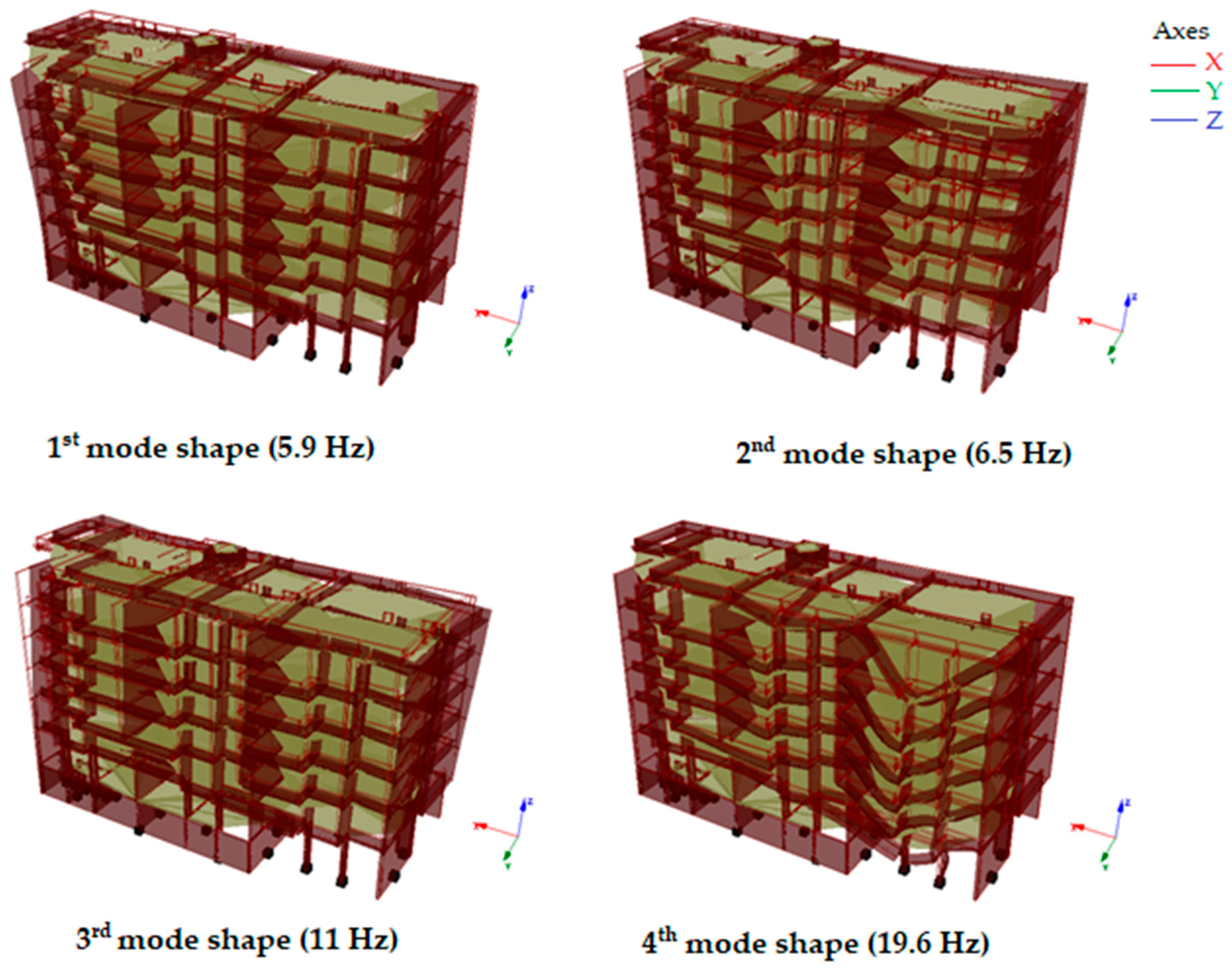
| n. | Mode Type | Freq. [Hz] | Effective Masses [%] | |||||
|---|---|---|---|---|---|---|---|---|
| Ux | Uy | Uz | Rx | Ry | Rz | |||
| 1 | 1st bending y | 5.90 | 1.87 | 43.23 | 0.00 | 25.59 | 0.62 | 15.96 |
| 2 | 1st torsional | 6.55 | 4.06 | 20.07 | 0.10 | 12.64 | 1.01 | 41.82 |
| 3 | 1st bending x | 11.06 | 56.46 | 0.00 | 0.06 | 0.00 | 17.24 | 5.14 |
| 4 | 1st bending z | 19.65 | 0.01 | 0.33 | 14.26 | 4.03 | 6.62 | 0.09 |
| Earthquake | Mw | Epicenter Coord. | Station | Id. |
|---|---|---|---|---|
| Valparaíso 1985 | 8.0 (CSN) 7.4 (USGS) | 33.207° S 71.663° W | Melipilla San Isdro | EQ1 EQ2 |
| Bío-Bío 2010 | 8.8 (CSN) 8.8 (USGS) | 36.122° S 72.898° W | Angol Concepción San Pedro Constitucion Llolleo | EQ3 EQ4 EQ5 EQ6 |
| Coquimbo 2015 | 8.4 (CSN) 8.3 (USGS) | 31.573° S 71.674° W | El Pedregal Tololo San Esteban | EQ7 EQ8 EQ9 |
| Valparaíso 2017 | 6.9 (CSN) 6.9 (USGS | 33.073° S 72.051° W | Torpederas | EQ10 |
| Rule | [s] | [s] | ||||
|---|---|---|---|---|---|---|
| EE—Equation (5) | 0.17 | 0.09 | 3.36 | 4.73 | 6.1 | 11.7 |
| EC8—Equation (7) | 0.17 | 0.09 | 3.36 | 4.73 | 2.79 | 4.16 |
| ASCE—Equation (8) | 0.17 | 0.09 | 3.36 | 4.73 | 2.8 | 3.94 |
| Analysis | Peak Top Displacement (m) | Interstory Drift (%) | ||
|---|---|---|---|---|
| X dir. | Y dir. | X dir. | Y dir. | |
| MRSA (not amplified) | 0.0011 | 0.0025 | 0.0083 | 0.0184 |
| MRSA amplified by Equation (6) | 0.0068 | 0.0287 | 0.0505 | 0.2152 |
| MRSA amplified by Equation (8) | 0.0031 | 0.0102 | 0.0231 | 0.0765 |
| MRSA amplified by Equation (9) | 0.0038 | 0.0116 | 0.0278 | 0.0869 |
| LTHA (average) | 0.0066 | 0.0193 | 0.0597 | 0.1352 |
| NLTHA (average) | 0.0204 | 0.0450 | 0.1422 | 0.3240 |
| Analysis | for Peak Top Displacement (%) | for Interstory Drift (%) | ||
|---|---|---|---|---|
| X dir. | Y dir. | X dir. | Y dir. | |
| MRSA (not amplified) | −94.6 | −94.4 | −94.2 | −94.3 |
| MRSA amplified by Equation (6) | −66.7 | −36.2 | −64.5 | −33.6 |
| MRSA amplified by Equation (8) | −84.8 | −77.3 | −83.8 | −76.4 |
| MRSA amplified by Equation (9) | −81.4 | −74.2 | −80.5 | −73.2 |
| LTHA (average) | −67.6 | −57.1 | −58.0 | −58.3 |
Publisher’s Note: MDPI stays neutral with regard to jurisdictional claims in published maps and institutional affiliations. |
© 2022 by the authors. Licensee MDPI, Basel, Switzerland. This article is an open access article distributed under the terms and conditions of the Creative Commons Attribution (CC BY) license (https://creativecommons.org/licenses/by/4.0/).
Share and Cite
Porcu, M.C.; Vielma Pérez, J.C.; Pais, G.; Osorio Bravo, D.; Vielma Quintero, J.C. Some Issues in the Seismic Assessment of Shear-Wall Buildings through Code-Compliant Dynamic Analyses. Buildings 2022, 12, 694. https://doi.org/10.3390/buildings12050694
Porcu MC, Vielma Pérez JC, Pais G, Osorio Bravo D, Vielma Quintero JC. Some Issues in the Seismic Assessment of Shear-Wall Buildings through Code-Compliant Dynamic Analyses. Buildings. 2022; 12(5):694. https://doi.org/10.3390/buildings12050694
Chicago/Turabian StylePorcu, Maria Cristina, Juan Carlos Vielma Pérez, Gavino Pais, Diego Osorio Bravo, and Juan Carlos Vielma Quintero. 2022. "Some Issues in the Seismic Assessment of Shear-Wall Buildings through Code-Compliant Dynamic Analyses" Buildings 12, no. 5: 694. https://doi.org/10.3390/buildings12050694
APA StylePorcu, M. C., Vielma Pérez, J. C., Pais, G., Osorio Bravo, D., & Vielma Quintero, J. C. (2022). Some Issues in the Seismic Assessment of Shear-Wall Buildings through Code-Compliant Dynamic Analyses. Buildings, 12(5), 694. https://doi.org/10.3390/buildings12050694