New Optimal Supply Air Temperature and Minimum Zone Air Flow Resetting Strategies for VAV Systems

Abstract

Buildings account for a large portion of the total energy use in the US; therefore, improving the operation of typical variable-air-volume (VAV) systems in buildings can provide a tremendous economic opportunity. ASHRAE Guideline 36 recommends a resetting strategy for supply air temperature (SAT) for VAV systems based on outside air temperature. However, this strategy may not produce optimal performance, particularly when simultaneous cooling and heating occurs in zones. In addition, there is no strategy recommended in the Guideline to reset the zone minimum airflow set point in a single-duct VAV terminal unit with reheat, although this setpoint has a great impact on zone reheat requirements and ventilation efficiency. Thus, this paper introduces new strategies to reset both the SAT and zone minimum airflow rate set points to improve the efficiency of typical VAV systems. The strategies were tested under various conditions through experiments performed in fully instrumented VAV systems located in the HVAC lab at the University of Cincinnati. The experiments were conducted on a chilled-water VAV system that serves three controlled zones with hot-water reheat VAV boxes controlled by a typical commercial BACnet web-based building automation system BAS. The simulation studies were performed using the building energy simulation software EnergyPlus to evaluate the strategies at a larger scale in various locations. The simulation results show that the proposed resetting strategies can provide fan energy savings between 1.6% and 5.7% and heating load savings between 7.7% to 33.7%, depending on the location. The laboratory testing shows that the proposed strategies can provide stable control performance in actual systems as well as achieving the anticipated reheat and fan energy savings. The result offers significant improvements that can be implemented in the Guideline for single-duct VAV system operation and control.

1. Introduction

Buildings are among the major consumers of global energy. As a matter of fact, this sector accounts for approximately 40 percent of the energy consumed in the United States, which is more than the amount of energy used by industry and transportation. Therefore, improving the energy efficiency of these buildings can reduce the total energy use and associated building carbon dioxide emission [1,2,3]. Building HVAC systems accounts for a large portion of a building’s energy consumption. Amongst different types of HVAC system, variable-air-volume (VAV) systems are used in most large-scale buildings. Therefore, any enhancement in the operation of typical VAV systems can provide both energy and cost-saving opportunities [4,5,6]. Hence, several studies have investigated different optimization strategies to achieve better energy efficiency in VAV systems. For example, some researchers focused on the optimum set points of one or several local-loop controllers. Wang and Song proposed the optimization of the supply air temperature during the economizer cycles, which can minimize energy costs [7]. On the other hand, Zhu et al. proposed an adaptive artificial neural-network-based control for the supply air temperature, which was tested in a pilot HVAC system to evaluate efficiency [8]. Taylor improved the VAV system efficiency by resetting the duct static pressure setpoint [9]. In another study, Taylor introduced a trim-and-response logic to reset the supply air temperature and duct static pressure setpoints [10]. Nassif offered improvements for the trim-and-response logic to enhance the system’s response to any changes in conditions [11]. Other studies have been performed to develop model-based optimization methods to optimize the overall performance of the VAV system instead of just one subsystem [5,12]. For instance, Seong et al. introduced a model-based method to optimize airside and waterside variables [13]. Talib and Nassif introduce a data-based optimization engine to improve the operation of chilled water and DX systems, including system- and zone-level setpoints [14]. Kim et al. proposed two control algorithms considering temperature and humidity as the factors of the indoor environment to maintain the occupant comfort while lowering the energy consumption in conventional HVAC systems [15]. Other studies are based on the optimization and control of HVAC systems following different modeling techniques and methods [16,17,18,19]. Unfortunately, these methods require accurate models with a high level of computation, and they are difficult to implement in real control systems. Even if these controls are implemented, their performance depends significantly on the accuracy of the models. Alternatively, ASHRAE Guideline 36 on high-performance operation sequences [20] introduces easy-to-implement, rule-based methods and control sequences for the operation of HVAC systems that are intended to maximize their energy efficiency, improve their performance, provide control stability, and allow real-time fault detection and diagnostics. The guideline recommends a trim-and-response method to reset the supply air temperature (SAT) set point for a multi-zone VAV system based on readings from zone cooling loops. The guideline recommends resetting the SAT linearly as a function of outside air temperature (OAT). When the building has zones mostly in cooling, as in interior zones, resetting the SAT based on OAT, as proposed by the Guideline, may not produce the best performance. This study did not address typical single-duct VAV terminal units, and the study did not test the methods in the real control systems to verify whether the control works properly in the real control system. Another issue is that the Guideline did not propose how to reset the minimum airflow rate set point in zones that are not equipped with CO₂ sensors. There is no clear guideline as to what the minimum flow rate setpoint should be. Typically, the setpoints are set to be 20–30% of design and kept constant during operation. The zone minimum airflow set point in a single-duct VAV terminal unit with reheat has a significant impact on zone reheat requirements and ventilation efficiency. Lowering the setpoint reduces the zone reheat requirements but reduces the ventilation efficiency, thereby increasing the ventilation load on the cooling and heating equipment. When the economizer is enabled, during the full or partial free cooling mode, a large amount of fresh air is introduced into the system to maintain the supply air temperature at its setpoint. This amount is typically greater than the required minimum ventilation; consequently, the setpoint can be lowered to reduce the reheat requirement without any effect on the ventilation load. Nassif et al. proposed a new resetting method for the minimum zone airflow rate set point, but the study assumed that the supply air temperature was constant, and the study overlooked the interaction between the SAT and the zone minimum airflow rate setpoints [21]. Thus, to address these challenges, this paper introduces integrated two control strategies that reset both the SAT and the minimum airflow rate set point for a single-duct multi-zone VAV system and evaluate the methods in simulation and real control systems. These strategies are easy to implement in real systems and can improve the efficiency of typical VAV systems.

1.1. Resetting Control Strategies

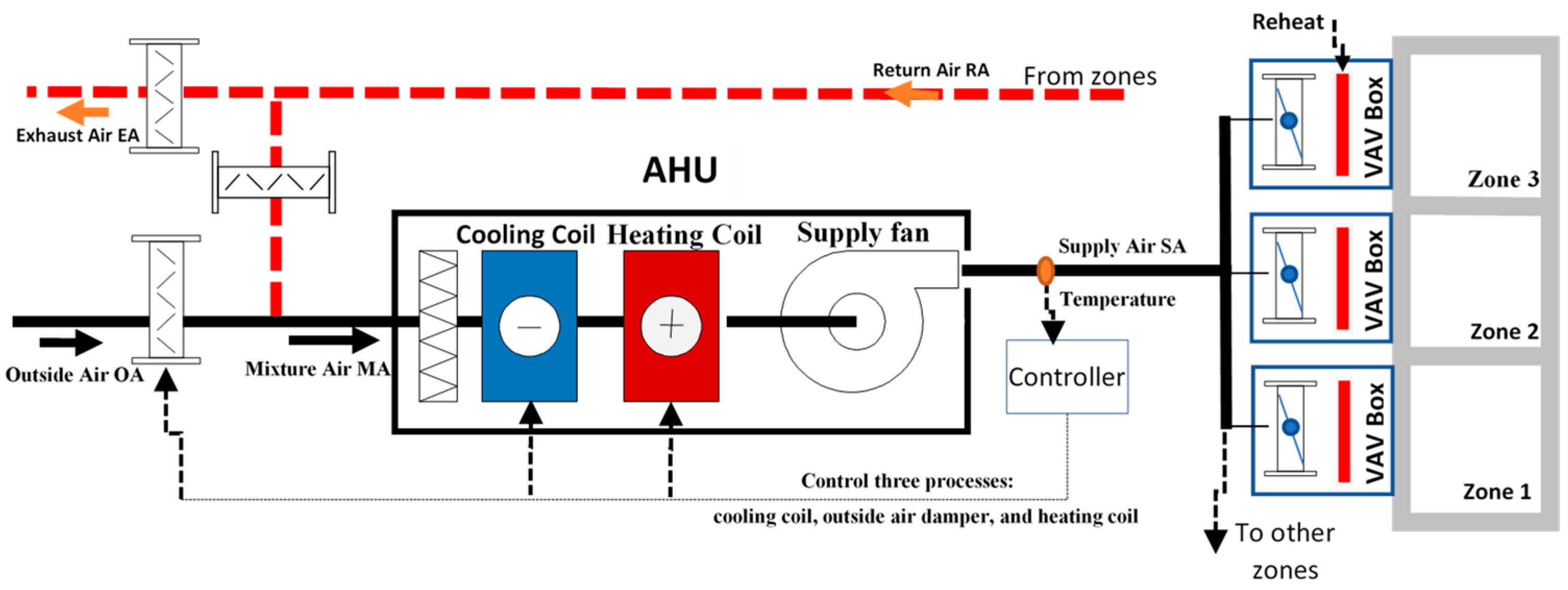
As shown in Figure 1, a typical VAV system has the following major control loops: space control loops, supply air temperature SAT control loop, and duct static pressure control loop. The space air temperature is typically controlled through a cascade control loop. One loop used is to determine the air flow rate setpoint that maintains the space air temperature. The other loop is used to control the VAV box damper that maintains the airflow rate at its set point. The duct static pressure control loop is used to maintain the static duct pressure at its set point by modulating the fan speed.

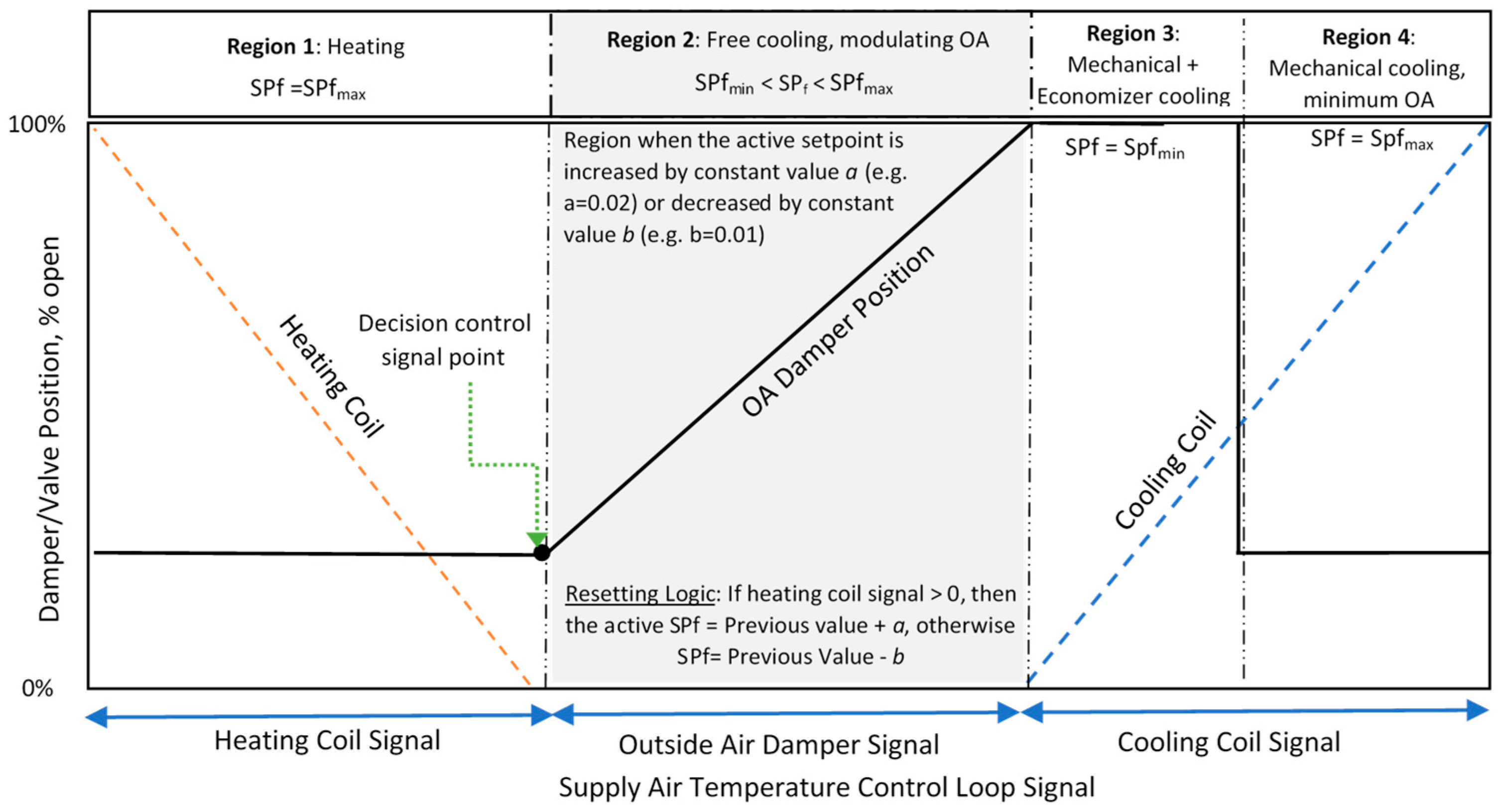
The supply air temperature control is used to maintain the supply air temperature at its set point. Depending on the air handling unit’s AHU operating states, the supply air temperature (SAT) is typically controlled in sequence by three separate controlled devices: cooling coil valve, outside air (OA) damper, and heating coil valve. Figure 2 shows four AHU operating states or regions, as follows. (1) Region 1—heating: when the SAT is maintained by modulating the heating coil valve position and OA damper is at the minimum position. (2) Region 2—free cooling and modulating OA: when the SAT is maintained by modulating the OA damper position. (3) Region 3—mechanical and economizer cooling: when the OA damper is fully opened, and the SAT is maintained by controlling the cooling coil valve position. (4) Region 4—mechanical cooling and minimum OA: when the OA damper is at the minimum position, and the SAT is maintained by controlling the cooling coil valve position.

1.2. Minimum Zone Airflow Rate SetPoint

Guideline 36 does not propose how to reset the minimum airflow rate set point in zones that are not equipped with CO₂ sensors. Since there is no clear guideline on what the minimum flow rate setpoint should be, the minimum zone airflow rate setpoint is typically set to be 20–30% of the design airflow (referred to, in this study, as the maximum value of the setpoint SPf_max). Without the application of a resetting control strategy, the active minimum airflow rate setpoint (referred to, in this study, as the setpoint for flow SPf) is kept constant during the operation (SPf = SPf_max). This research introduces a new strategy to reset the active minimum airflow rate setpoint (SPf) at every time step (e.g., 5 min) between the design value (SPf_max) and the lowest possible value (SPf_min). The lowest possible value of the setpoint (SPf_min) is equal to and greater than the ventilation required in the breathing zone or minimum airflow required for VAV box control stability.

The recommended set point (SPf) depends on the operating states of the AHU, as shown in Figure 2. In region 1, the active setpoint (SPf) should be kept at the design maximum value (SPf_max), as reducing the setpoint increases the amount of OA required for ventilation and, consequently, the AHU heating requirement. In region 2, when the SAT is maintained by modulating the OA damper, the system introduces less than 100% fresh air, which may be higher than the minimum ventilation requirement, so the supply air is rich in fresh air, and the setpoint can be reset to lower than the maximum value (SPf_max). Ideally, the setpoint can be optimally selected to make the required OA for ventilation near the OA introduced by the outdoor damper to maintain the SAT at its set point, in which case, there is no need for mechanical cooling or heating. However, this can be difficult to apply in real systems. A simple and easy-to-implement resetting strategy is to use the heating capacity control signal as an indicator to change the set point. Any time the heating capacity signal (or heating valve position) is higher than zero (or a threshold), the active SPf should be increased by a certain value (e.g., a = 0.02 or 2% of the design value). Otherwise, the setpoint decreases by a certain value b (e.g., b = 0.01 or 1%). There is no need to reset the minimum airflow rate setpoints in zones with airflow rates higher than the SPf_max. Any zones with airflow rates equal to or lower than the SPf_max are called critical zones, and the reset takes place only in those zones. In direct-expansion, DX-packaged units, the heating signal (if furnace or heat-pump) can be used instead. In region 3, the SPf should be kept at the SPf_min that is equal to the ventilation required in the breathing zone. In region 4, the SPf should be kept at the SPf_max. Decreasing the setpoint may increase the ventilation requirement and, consequently, the cooling load.

1.3. Supply Air Temperature Setpoint

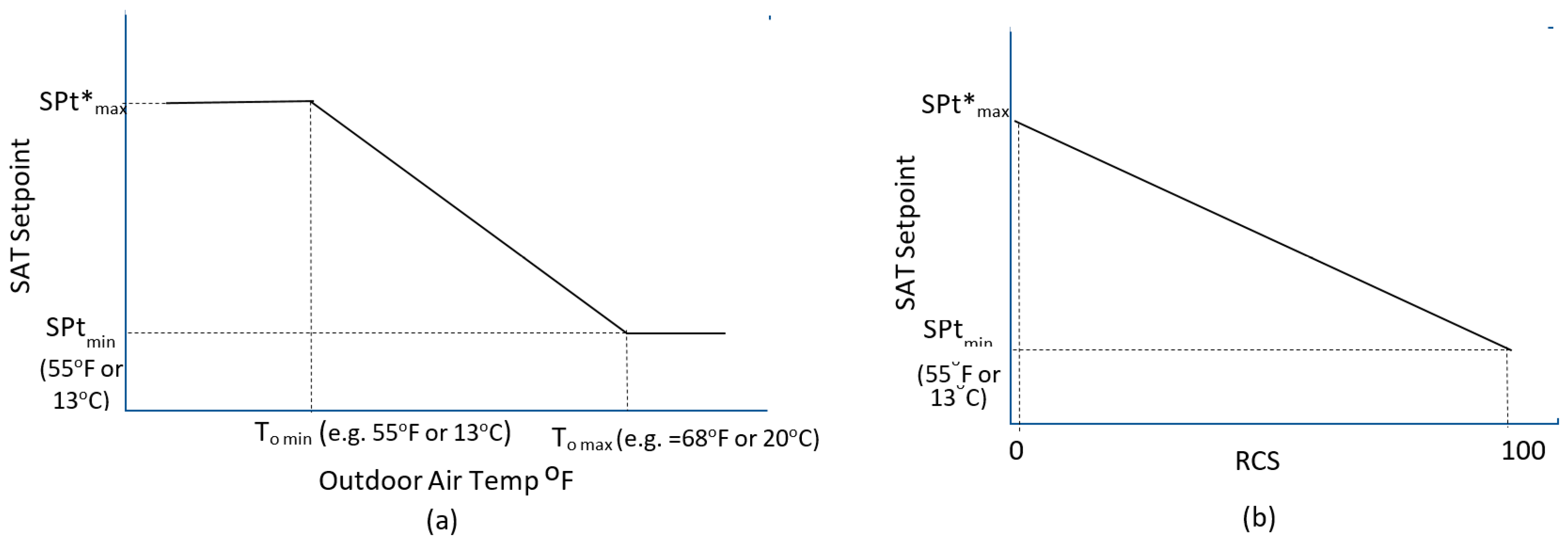
The Guideline 36 resetting algorithm resets the SAT setpoint (referred to, in this study, as the set point for temperature SP_t) linearly between a fixed minimum value SPt_min (e.g., 55 °F or 13 °C) and an adjusted maximum value SPt*_max as a function of outside air °F temperature (OAT), as shown in Figure 3a. The resetting algorithm is based on a predefined minimum change-point outside air temperature To_min (e.g., 55 °F or 13 °C) and the maximum change-point outside-air temperature To_max (e.g., 68 °F or 20 °C). The active maximum value SPt*_max is dynamically adjusted using the trim-and-response algorithm to ensure that the SAT is low enough to meet the required cooling load in the critical zone (s) by keeping the cooling control signal lower than a predetermined value (e.g., less than 95%).

Even when it is cold, there may be several zones in cooling, and the SAT resetting based on OAT proposed by the Guideline may not produce the best performance. Thus, the proposed strategy uses the zone cooling or heating control loops instead of the OAT to count the number of zones in cooling or heating at any time. If the zone is in cooling or deaband, the zone value ZV is assigned to be one; otherwise, it is zero. The SAT resetting cooling signal RCS is then calculated as follows:

$$RCS={\displaystyle \sum }_{i=1}^n{a}_{i}Z{V}_i$$

Here, n is the number of zones. The term a is a factor to give a weight for zone i. The value of a_i can be determined from the design airflow rate or actual readings. In this paper, a_i is calculated by the ratio of the design zone airflow rate to the sum of the design zone airflow rates. The sum of a_i should be 1. The RCS should then vary from 0 to 1 (0 to 100%). If no zones are in cooling, the RCS is zero. If all zones are in cooling, it becomes 1 (100%). The SAT is reset based on the RCS, as shown in Figure 3b. The maximum value of the SAT setpoint SPt*_max is dynamically adjusted using the same trim-and-response algorithm recommended in the Guideline to ensure that the SAT is cold enough to meet the cooling load in critical zone(s).

2. Simulation Study

To evaluate the proposed strategies, a 5000 ft² (463.6 m²) office building was selected from EnergyPlus example files. The detailed building description can be found in the comment line of the IDF example file of EnergyPlus (5ZoneVAV-Pri-SecLoop) [22]. The building had a 100 ft × 50 ft (30.5 m × 15.2 m) rectangular shape and five zones: four exterior and one interior. A single-duct VAV box with hot water was used instead of a fan-powered VAV box. Five resetting strategies were investigated and programmed in the Energy Management System EMS of EnergyPlus. The strategies are listed in

Table 1. Investigated resetting strategies.

Strategies	Notes	(Set Point for Temp.) SPt	(Set Point for Flow) SPf
Strategy I (S1)	Keep SPt constant at the lowest value to save fan energy power	SPt = 13 °C (55.4 °F)	SPf = SPfmax
Strategy II (S2)	Reset SPt based on OAT (but SPtmax = constant)	SPt = Vary (see Figure 3a)	SPf = SPfmax
Strategy III (S3)	The SAT strategy recommended in Guideline 36	SPt = Vary (see Figure 3a)	SPf = SPfmax
Strategy IV (S4)	Proposed SAT reset	SPt = Vary (see Figure 3b)	SPf = SPfmax
Strategy V (S5)	Proposed (SPt + SPf) reset	SPt = Vary (see Figure 3b)	SPf = Vary (see Figure 2)

. Strategy S1 was the simplest: it kept the SAT setpoint (SPt) constant at the lowest value of 55.4 °F (13 °C) to save fan energy power. Strategy S2 reset the SAT setpoint (SPt) linearly as a function of OAT from the minimum value (SPt_min) of 55.4 °F (13 °C) to the nonadjustable or fixed maximum value SPt_max of 64.4 °F (18 °C). Strategy S3 is the strategy recommended in Guideline 36. SPt is reset based on OAT from the minimum value (SPt_min) of 55.4 °F (13 °C) to the adjustable (active) maximum value (SPt*_max). The maximum active value is adjusted from 55.4 °F (13 °C) to 64.4 °F (18 °C) using the trim-and-response algorithm to ensure there is no cooling control signal in any zone greater than 95%. Strategy S4 is the proposed SAT resetting strategy, as presented in Figure 3b. Strategy S5 is the proposed SAT strategy, as presented in Figure 3b, but in conjunction with the proposed minimum zone airflow rate resetting algorithm presented in Figure 2. For all the strategies that are based on OAT, To_max was set to be 68 °F (20 °C) and To_min was set to be 50 °F (10 °C). For all the strategies, the minimum and maximum SAT setpoints were 55.4 °F (13 °C) and 64.4 °F (18 °C), respectively. The maximum values of the minimum zone airflow rates (SPf_max) were set to be 30% of the design zone airflow rates. In strategies S1–S4, the minimum zone airflow rate setpoint SPf is kept constant at the maximum value (SPf = SPF_max). The required OA for ventilation is calculated based on ASHRAE Standard 62.1 multi-zone VAV ventilation procedure [23].

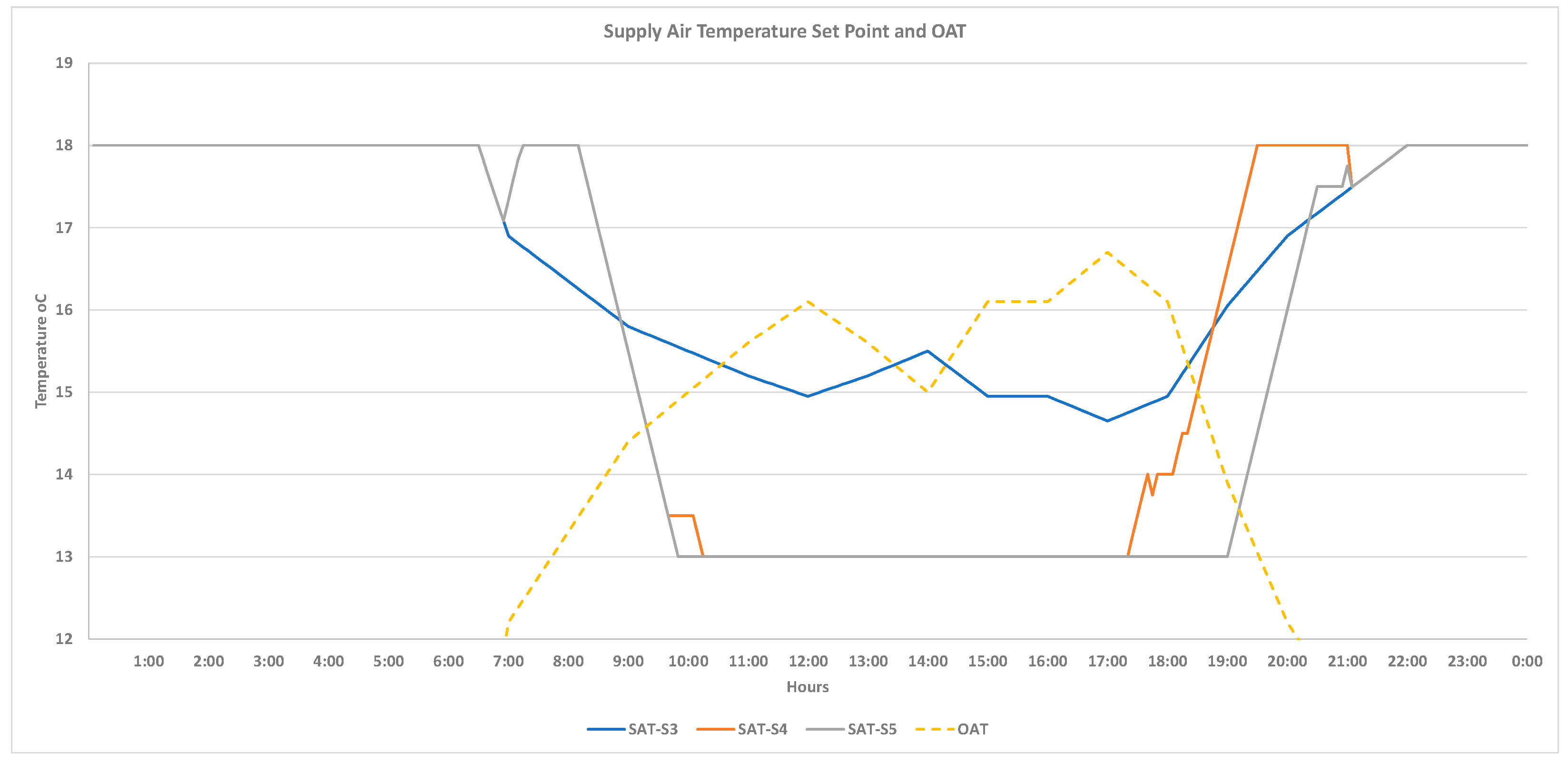
The simulation runs for all five strategies above, in several locations (Chicago, Tampa, Washington DC, Golden, and San Francisco). However, for discussion, the results for one day in spring in Chicago and three strategies (S3, S4, and S5) are presented in Figure 4, Figure 5, Figure 6, Figure 7, Figure 8 and Figure 9. The SAT and OAT for that day are shown in Figure 4. Figure 5 shows the total zone reheat requirement (the sum of the reheats in all the zones). 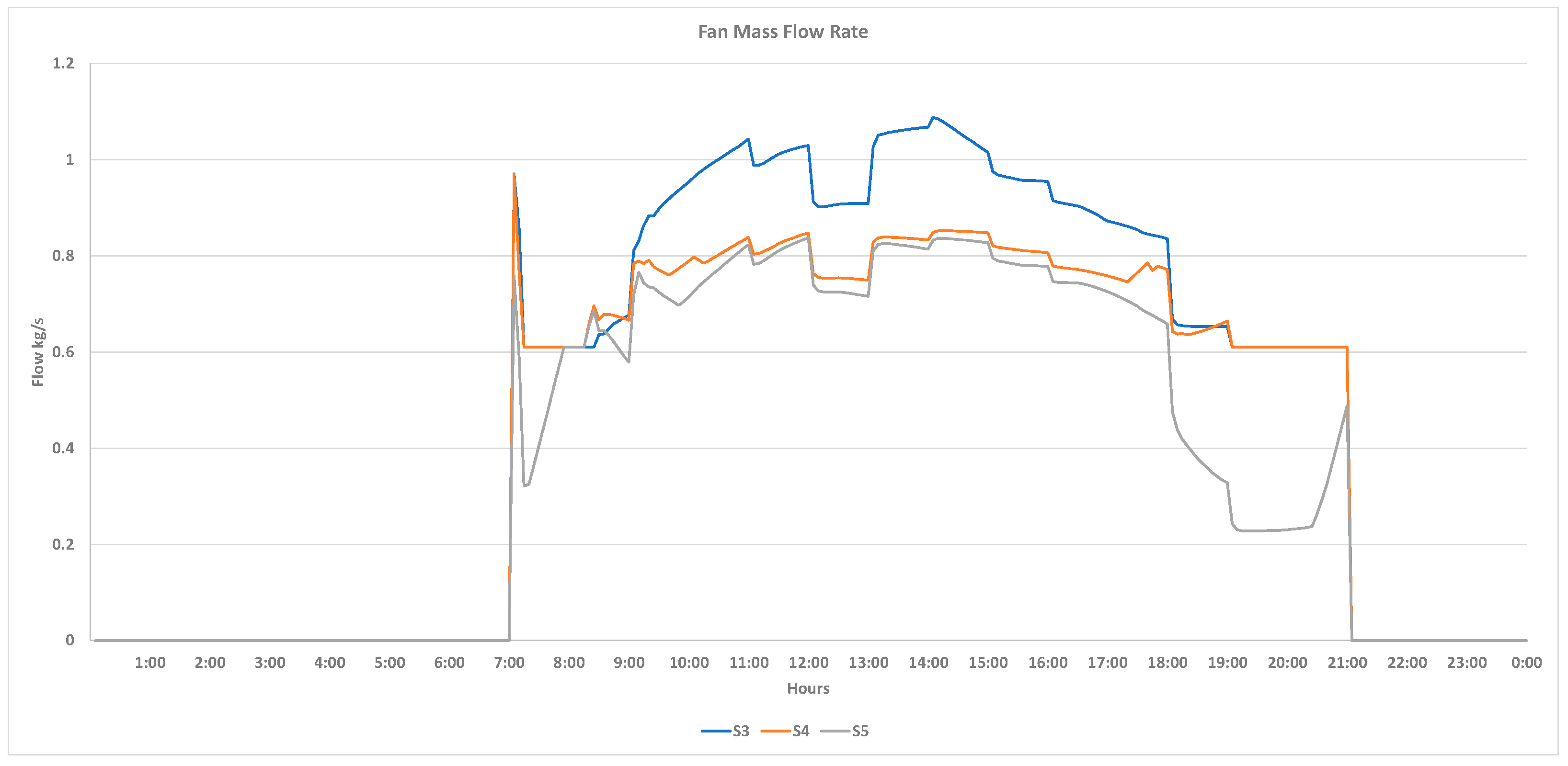Figure 6 and Figure 7 show the mass flow rate and fan power, respectively. 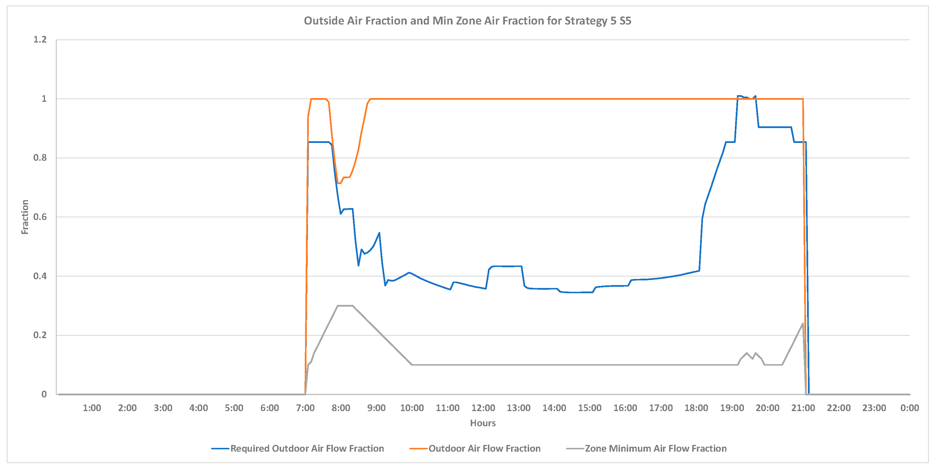Figure 8 and Figure 9 show the OA introduced to maintain the SAT at its set point and the required OA for ventilation for only both strategy S4 and strategy S5, respectively. The required OA for ventilation is calculated based on ASHRAE standard 62.1. The minimum zone airflow rate setpoint is also illustrated in Figure 9 for strategy S5. It is constant at 0.3 for other strategies.

Between 7:00 and 9:00, since most zones were heating and the proposed strategies S4 and S5 reset the SAT setpoint based on zone cooling requests, these strategies kept the SAT at approximately the maximum value of 64.5 °F (18 °C) (see Figure 4). However, S3, which is based on OAT, reset the SAT setpoint to lower than 64.5 °F (18 °C). In this case, the reheat requirement for S3 was larger than for S4 and S5 (see Figure 5). The reheat requirement was reduced further when S5 was applied as the strategy dropped the minimum zone airflow rate setpoint below the maximum value of 0.3 (30% of design flow) (see Figure 9). Before 8:00, the introduced economizer OA approached the required OA for ventilation and it no longer maintained the SAT at its set point. The SAT was then controlled by the system heating coil valve (moving from region 2 to region 1, as shown in Figure 2). As the valve slightly opened (not shown here), S5 responded by increasing the minimum airflow rate setpoint gradually over time as long as the heating was activated. After 8:00, S5 dropped the setpoint back to the minimum value as no heating was needed and the OA introduced maintained the SAT at its set point (back to region 2).

Between 9:00 and 18:00, all the zones cooled. S4 kept the SAT setpoint at 55.4 °F (13 °C), whereas S3 reset the set point to around 59 °F (15 °C) as it is based on OAT (see OAT profile in Figure 4). During this period, there were no reheats required in the zones and the lowering of the SAT by S4 reduced the supply airflow rate and, subsequently, the fan power, as shown in Figure 6 and Figure 7. S5 did the same as S4, but by dropping the minimum airflow rate setpoint to the minimum value of 0.1, as 100% OA was introduced, as shown in Figure 9, and, consequently, S5 further reduced the supply airflow rate and fan power. Between 18 and 19, S5 kept the minimum airflow rate at around 0.1 and, due to this low zone airflow rate, the changes to the heating from the cooling in the zones were delayed compared to S3 and S4, and the SAT setpoint stayed at 55.4 °F (13 °C) for a longer period, saving fan power with no negative effect on reheating requirement. After 19:00, as more zones heated, S4 and S5 reset the SAT setpoint gradually to a higher value, even higher than the value for S3. During this period, the reheat requirement when S4 was applied was lower than the reheat requirement when S3 was applied. S5 reduced the reheat requirements and fan power even further. Between 19:00 and 20:00, the 100% OA required to maintain the SAT at its set point became less than the required OA for ventilation and the heating coil valve had to open to maintain the SAT. S5 then reset the minimum set point to a higher value, keeping the introduced OA near the required OA. This result shows that the proposed S4 reduced the heating requirement and fan power compared to S3. However, S5, by including the minimum airflow setpoint reset, further reduced the reheat requirement and the fan power while providing the required OA.

This section shows the annual results for various locations.

Table 2. Annual energy fan consumption and loads for baseline (Strategy S3).

Location	Reheat Load kWh	System Heating Load kWh	Total Heating Load kWh	Fan Power kWh	Cooling kWh
Golden, CO	4507.1	1807.3	6314.4	6408.2	17,159.4
San Francisco, CA	2411.6	634.8	3046.4	5105.1	13,118.4
Tampa, FL	2601.1	262.2	2863.3	5207.5	64,568.1
Washington, DC	4190.4	3084.8	7275.2	5159.7	30,432.2
Chicago, IL	5572.7	4572.0	10,144.7	5184.4	24,284.6

shows the annual fan energy consumptions and heating and cooling loads for the baseline, Strategy S3.

Table 3. Percentage changes of fan energy consumption and cooling and heating loads from the baseline, Strategy S3 (positive sign is energy or load saving or reduction).

Location	Reheat				System Heating				Total Heating				Fan Power				Cooling
	S1	S2	S4	S5	S1	S2	S4	S5	S1	S2	S4	S5	S1	S2	S4	S5	S1	S2	S4	S5
Golden, CO,	−47.5%	10.4%	−0.9%	8.4%	49.6%	5.2%	7.5%	4.6%	19.7%	5.9%	1.5%	7.3%	4.9%	0.0%	4.1%	5.7%	−7.8%	3.5%	−2.3%	−2.1%
San Francisco, CA,	103.3%	0.0%	12.2%	43.6%	93.5%	0.0%	17.8%	4.3%	2.3%	0.0%	5.9%	33.7%	4.1%	0.2%	3.6%	5.4%	29.6%	0.1%	10.6%	18.1%
Tampa, FL,	−28.1%	0.1%	41.9%	68.9%	77.7%	0.2%	−5.6%	2.1%	18.4%	0.1%	37.6%	62.4%	0.6%	0.1%	0.2%	1.6%	−1.4%	0.0%	5.1%	7.9%
Washington, DC,	−47.9%	0.1%	5.4%	15.1%	40.3%	0.9%	7.1%	7.6%	10.5%	0.3%	6.1%	11.9%	3.5%	0.3%	2.7%	4.0%	−3.2%	0.0%	3.1%	4.2%
Chicago, IL,	−37.3%	0.1%	2.4%	8.8%	32.5%	0.5%	7.3%	7.3%	−5.8%	0.2%	4.6%	8.1%	3.7%	0.3%	2.9%	4.0%	−4.9%	0.0%	1.8”	2.2%

shows the energy or load change as a percentage of the baseline (Strategy S3). The change was calculated by subtracting the energy use or load for any investigated strategy from the baseline divided by the baseline energy use or load. The positive value means energy use or load saving or reduction from the baseline. The negative value means energy use or load increase from the baseline.

As strategy S1 kept the SAT at 55.4 °F (13 °C), the annual fan energy consumption was lower than the baseline but the reheat and total heating requirements were greater. For example, in Chicago, the fan power saving (reduction) was +3.7%, and the total heating increase was −5.8%. S2 performed largely the same as S3 in most locations, except that in Golden, the heating and cooling loads were reduced by S2. However, S3 ensured there was no zone starving for airflow in cooling mode. The proposed strategy, S4, significantly reduced the total heating loads and fan energy consumption in all the locations. For instance, in Chicago, the total heating load reduction was 4.6%, and the fan energy use reduction was 2.9% from the baseline, S3. With minimum zone airflow rate reset, S5 can further reduce total heating requirements and fan energy uses. For instance, in Chicago, the total heating load reduction was 8.1%, and the fan energy use reduction was 4% from the baseline, S3. S4 and S5 reduced the cooling loads in some locations but increased the load in other locations. A large increase occurred in San Francesco, where the cooling load increased by about −10.6%, as maintaining lower SAT during economizer mode reduces the number of hours of full free cooling. For instance, if the OAT is around 60.8 °F (16 °C) and S4 or S5 sets the SAT set point at 55.4 °F (13 °C), the cooling coil should cool the supply of 100% OA from 60.8 °F (16 °C) to 55.4 °F (13 °C). However, the cooling loads can drop to near zero if the SAT is set to be 60.8 °F (16 °C). Nevertheless, this increases the fan energy use, so there is a balance between fan and cooling energy uses. To reduce the cooling load during economizer mode while increasing the fan power, the proposed strategy S4 or S5 can only be modified by resetting the SAT setpoint linearly as a function of OAT in the range between 55.4 °F and 62.6 °F (13 °C and 17 °C). Doing this modification, the cooling coil load will reduce (not increase) by 2.5% and the fan power will reduce by 2% (instead of the original 5.4%) from the baseline.

3. Laboratory Deployment

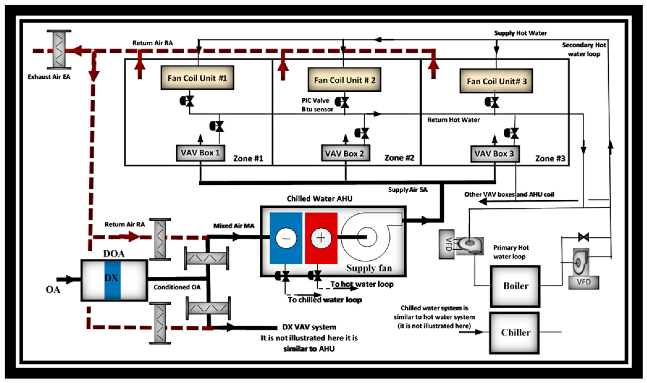
The Guideline 36 strategy, S3, the proposed SAT strategy S4, combined with the proposed SAT reset and minimum zone airflow rate reset strategy, S5, was implemented in a real chilled-water VAV system installed in the HVAC lab at the University of Cincinnati. Figure 10 shows the photos of the laboratory and Figure 11 shows a simple schematic of the laboratory. It contains various types of HVAC system: chilled-water and DX VAV systems, four-pipe fan coil units, and variable refrigerant-flow VRF systems serving three environmentally controlled zones. A chiller and electric boiler deliver chilled and hot water to the chilled water VAV system, fan coil units, and hot-water VAV box reheat coils. The outside air entering the VAV systems is conditioned by a dedicated DX coil located on the OA intake (DOA). The systems are controlled by a typical commercial BACnet web-based building automation system BAS. The temperature difference and water flow rates are measured across all fan coil units, reheat coils, and AHU coils.

Multiple tests were initially performed by controlling the OAT entering the unit through the DOA at different values, ranging from 45 °F (7.2 °C) up to 85 °F (29.4 °C), covering regions 1–4, as shown in Figure 2. When the economizer was disabled (region 4), all the strategies performed at the same level, the SAT set point was at the minimum value of 55 °F (12.7 °C), and the minimum zone airflow rate was at the maximum value (SPf_max). 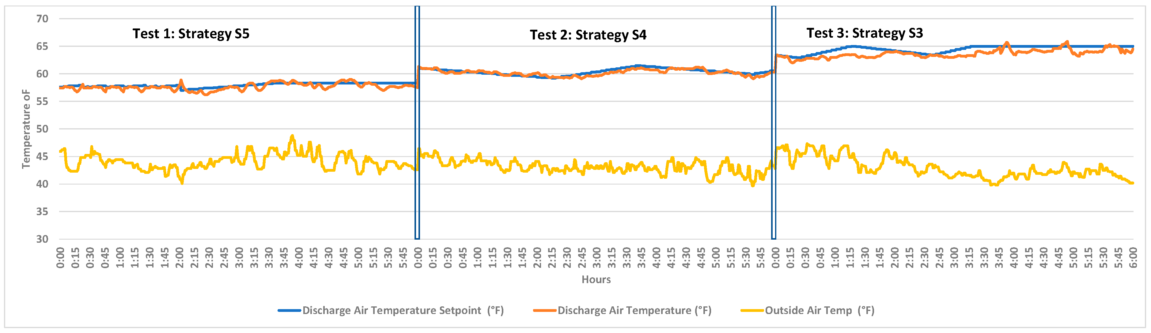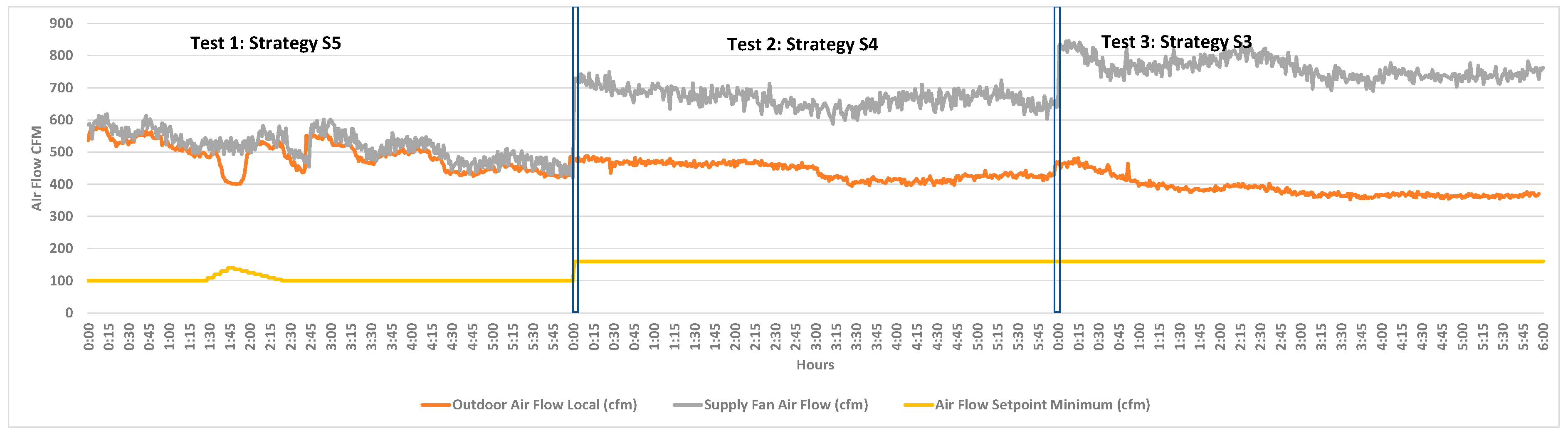When it was too cold outside and all the zones were heating (region 1), all the strategies also performed similarly, the SAT set point was at the maximum value of 65 °F (18.3 °C), and the minimum zone airflow rate was at the maximum value (SPf_max). Hence, this paper focuses on the evaluation of the strategies in region 3 and the transition area between regions 3 and 4. In these regions, the OAT needed to be approximately lower than 45 °F (7.2 °C) and the DX unit (DOA) could not achieve such a low temperature. Therefore, three tests were performed on three different nights from 11 am to 6 am, when the OAT was somewhat the same, as shown in Figure 12. The OAT sensor was located at the OA intake and read approximately 44 ± 3 °F (6.6 ± 1.6 °C) during those three tests. The first hour of the test, as this transition period, was excluded from the analysis. The first test, Test 1, was when strategy S5 was applied (both proposed SAT and minimum airflow rate resetting algorithms were included). The second test was when strategy S4 was applied (only the proposed SAT algorithm was included). The last test was for the baseline strategy S3, when the Guideline 36 SAT resetting strategy was applied. In Test 2 and Test 3, the minimum airflow rates are kept constant at 32% (i.e., 160 cfm). The design zone airflow rate for each VAV box was 500 cfm (236 L/s) and the design minimum zone airflow rate (SPf_max) was 160 cfm (75.5 L/s). The breathing ventilation per zone was 80 cfm (37.7 L/s). Since the VAV box was unable to control the zone airflow below 80cfm (37.7 L/s), the minimum setting value of the minimum zone airflow rate (SPf_min) was set at 100cfm (47.1 L/s) in Test 3, which was greater than the minimum ventilation requirement of 80cfm (37.7 L/s). All the control parameters and programs were kept the same as those installed by the controlling contractor. The only change was the addition of the strategies investigated in this paper and a new algorithm to calculate and control the minimum outside air flow rate setpoint, based on the ASHRAE standard 62 procedure. The fan coil units were used to add heat to zones representing “artificial” cooling loads at the rates of 5500 btu/h (1612 W), 1000 btu/h (293 W), and 0 btu/h for zone 1, zone 2, and zone 3 respectively. This was performed by controlling the hot water flow rate by the pressure-independent control water valve, and the hot water supply temperature was maintained at 130 °F (54.4 °C). These heats caused Zone 1 to cool and Zone 3 to heat. Zone 2 swung between cooling and heating, depending on the resetting strategies applied. The zone heating temperature set point was 72 °F (22.2 °C) and the zone cooling temperature setpoint was 74 °F (23.3 °C).

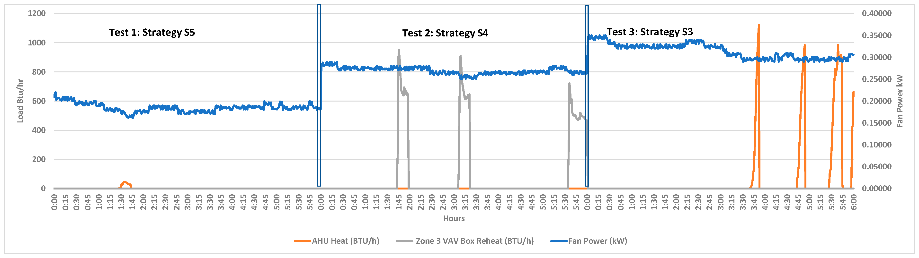
Figure 12, Figure 13 and Figure 14 show the experiment results for the three tests. As shown in Figure 13, strategies S3 and S4 kept the minimum airflow rate set points at 160 cfm (75.5 L/s), whereas S5 kept them near 100 cfm (47.1 L/s). S5 kept the OA introduced to maintain the SAT at its setpoint, somewhat similar to the required ventilation achieved by dropping the zone minimum airflow rate from the maximum value of 160 cfm (75.5 L/s) to 100 cfm (47.1 L/s). At around 1:30, the AHU heat was activated to maintain the SAT at its setpoint (transient from region 3 to region 4), and S5 increased the minimum set point incrementally by 10 cfm (4.7 L/s) every 5 min. When there was no heating required at the system level and the SAT could be maintained by OA (region 3), S5 reduced the minimum set point incrementally by 5 cfm (2.4 L/s).

In Test 1, as two zones (Zone 1 and 2) were cooling, S5 set the SAT setpoint at around 58 °F (14.4 °C). However, in Test 2, S4 maintained the SAT set point at around 62 °F (16.6 °C) as there was only one zone (Zone 1) cooling. The minimum airflow rate in Zone 2 was 160 cfm (75.5 L/s) in S4 (instead of 100 cfm in S5), this high flow caused Zone 2 to heat (more cold air supplied to the zone). S3 kept the SAT set point at around 64 °F (17.7 °C) as the OAT was around 45 °F (7.2 °C). As S4 kept the SAT colder than the SAT for S3, the fan airflow and power for S4 were lower than for S3. S5 further reduced the fan power due to two reasons: (1) the colder supply air that met the load in Zone 1 and (2) the lower zone airflow rates in Zone 2 and Zone 3 (100 cfm instead of 160 cfm). Comparing S5 with S4, a large reheat saving was obtained by S5 due to the lower minimum airflow rate. No reheat was required by S3 as this strategy kept the SAT at an elevated set point of 64 °F (17.7 °C) but the system heating increased. Indeed, in this case, the heating shifted from the reheat coil to the AHU coil. As a result, S5 required much less fan power and reheated. In another scenario, which is not presented here, in cases in which all the zones are heating, S5 will maintain the SAT at the maximum value of 65 °F (18.3 °C), whereas S3 may, or may not, maintain the SAT at the maximum value, which depends on the OAT. This may occur in the early morning in spring or fall, when the zones heat and the OAT rises very quickly, so that S3 may not maintain the SAT at the maximum value (see Figure 4, between 8:00–9:00 in the simulation section).

An additional result that is not presented in this paper is the case in region 2, in which the AHU heating was never activated, and the recommended strategy S5 always maintained the minimum zone airflow rate at the minimum value of 100 cfm (47.1 L/s) and the SAT at around 55 °F (12.7 °C) when all the cooling zones and large fan and reheat savings were consequently achieved.

4. Conclusions

Integrated SAT and minimum airflow rate resetting strategies are introduced in this paper in order to achieve better energy efficiency in buildings. The SAT strategy uses an algorithm to count the number of zones in the process of cooling or heating and uses this count to reset the SAT instead of relying only on the OAT. This method can create a better balance between fan power and heating requirement, compared to the strategy recommended in Guideline 36. The minimum airflow resetting strategy takes the AHU’s operating states and heating coil signal into account and determines the minimum airflow rate setpoint accordingly. Both strategies were evaluated in simulation and laboratory environments. The simulations were performed on an office building using EnergyPlus software; the strategies were programmed in the EMS of the software. The simulation results show that if both proposed strategies are implemented instead of the one in the Guideline, the fan energy savings are between 1.6% and 5.7%, and the heating load savings are 7.7% to 33.7%, depending on the locations. A cooling load saving can also be achieved, but this depends strongly on the location and the number of hours the system operates in free cooling mode. However, the cooling load can be reduced even in such a location by adjusting the proposed SAT algorithm to reset the SAT as a function of OAT only when the OAT is within the range of 55.4 °F to 62.6 °F (13 °C and 17 °C). The laboratory testing was performed in a full-scale chilled-water VAV system instrumented and controlled by a commercial BAS. The lab testing showed that the proposed strategies provide stable control performance in an actual system. The experiments also validate the results from the simulation and show reduced reheat requirements and fan energy savings. The proposed integrated SAT reset and minimum airflow rate control strategy show significant energy consumption. Therefore, they can be added and implemented as a part of the Guideline for better VAV system control.