Analytical Reliability Evaluation Framework of Three-Dimensional Engineering Slopes

Abstract

An analytical three-dimensional slope reliability evaluation framework was developed in this work independent of use of numerical simulations. The slope stability analysis was necessarily carried out by utilizing an extended three-dimensional Morgenstern–Price method, which was characterized by analytical formulations and competitive computational efficiency. Incorporation of the presented stability analysis method into response surface methodology led to an effective slope reliability evaluation framework. The applicability and superiority of this framework was examined and validated using a real complicated landslide case reported in practice, and a hypothetical slope example widely adopted in the literature. The impact of correlation coefficients and probability distribution patterns on the slope reliability assessment results was further addressed to derive additional benefits of this framework.

1. Introduction

The stability analysis on a two-dimensional (2D) cross-section of a real slope has been stated to be capable of giving reasonable and acceptable stability evaluation of three-dimensional (3D) slopes or excavations in terms of the factor of safety [1,2]. The wide applicability of 2D stability analysis is dependent on the implied plain-strain assumptions in fundamental theory. This applicability requires that the analyzed slope extends sufficiently in its width direction perpendicular to the analyzed cross-section and that the random variability of soil properties is not significant in the sliding mass. The end effect of slope geometry and probability effect of soil properties were gradually taken into account by performing 3D stability analysis and reliability analysis, with efforts to remove different hypotheses in the formulation of corresponding techniques [3,4]. Based on the limit equilibrium principle, the rigorous formulation for 3D slope stability analysis requires static force equilibrium and moment equilibrium on both the single column and the whole sliding mass in all directions. In addition, it includes a certain static condition of inter-column faces and a limit state of the slip surface with specific failure criterion. This generally renders the problem indeterminate by producing more unknowns than knowns, as described in [5,6].

Further, approaches to solve the indeterminacy of this problem can be classified based on three aspects as: (a) a reasonable compromise on force/moment equilibrium in single or more directions [7,8]; (b) the assumptions on the geometry of the sliding mass [9]; and, (c) efforts to introduce the simplified relationship of the inter-column forces or forces on column bases, in addition to complying with failure criterion [10]. Note that the combination of the foregoing aspects is commonly adopted in order to obtain the optimum balance between the acceptance degree and the computational consumption for the derived stability evaluation results [11].

Moreover, the kinematic movement analysis for the sliding mass is another alternative in order to perform the 3D slope stability evaluation. It is accomplished by applying the upper bound theorem in limit analysis [12,13], while the limit equilibrium formulation can be identified as the application of the lower theorem in limit analysis. Although an available extension has eliminated the column-partitioning technique manifesting in most of the limit equilibrium methods [14,15], the extending 3D column technique based on the 2D slice method is still attracting researchers’ attention due to its theoretically easy understanding and accessibility for engineers [16]. It should be noted that the extensions of the Morgenstern–Price (M-P) method [17] are reported mostly by highlighting the traits of fitting the slip surface with an arbitrary geometry and transforming this to other extensions by introducing the least number of possible simplifications in the earlier mentioned three aspects [18,19].

Apparently, consideration of the end effect for the 3D sliding mass would lead to the magnification of spatial variability for soil properties, which are inherently related to composition and structural diversity of soils. Slope reliability analysis was particularly developed to incorporate the above stochastic idea into the stability analysis of three-dimensional slopes. Numerical simulations, especially finite element modeling, were conventionally used to derive stability factors for three-dimensional slopes, which is necessarily required in slope reliability evaluation [20,21]. However, many sampling tools in reliability analysis (e.g., central point and checking point methods) can only be implemented based on the derivative information of performance functions [22,23], which is not available in numerical simulations. Their applicability to 3D slope reliability analysis is extremely limited due to the difficulty of establishing the slope performance function in explicit forms, which is a requisite condition to deduce derivative information.

In addition, the response surface method (RSM) proposed by Wong [24] stands out among others as having the flexibility of completing random sampling by finite element simulations and the capability of fitting the implicit performance function by polynomial functions around a certain checking point [25]. Through this transformation, the conventional reliability tools used in structural analysis are able to solve these explicit proxy performance functions in polynomial forms characterizing the failure probability of the sliding mass. In order to implement the reliability evaluation by RSM, based on the specific limit equilibrium method, the formulations deduced by 2D slice or 3D column methods were adopted to replace the finite element simulation without a clear physical formulation in the sampling process [26,27]. The finding is worth mentioning in these attempts, such that reliability analysis of a single determinate slip surface tends to give a less accurate slope failure probability than that with multiple potential slip surfaces, regardless of the increase in computational consumption. Chen and Zhu [28] thoroughly reviewed the application of RSM to slope reliability analysis and identified all these problems by classifying them into four categories, with suggestions on the selection of the appropriate RSM. The author examined the feasibility of slope reliability evaluation based on the 2D M-P method and the RSM in previous work [29]. Thus, the 3D extension for the 2D M-P method presented in the following paragraph was incorporated into the RSM to evaluate its applicability to be extended to 3D slope reliability analysis.

This paper presents the formulation of the 3D Morgenstern–Price Method (3DMPM), and examines its accuracy and effectiveness on a practical landslide case with complex geometry, and a hypothetical spherical slope example with external evaluation results, both of which are well reported in the literature. The implementation of the incorporation this 3DMPM technique into the RSM is demonstrated so as to examine its applicability in 3D slope reliability evaluation based on the hypothetic spherical slope example. Additionally, the impact of stochastic properties for slope soils and their priority in the cross-influence evaluation of the slope reliability condition was explored. This work may provide insights into the impact of soil stochastic characteristics on slope failure probability and offer an alternative for 3D slope reliability evaluation.

2. Implementation of 3DMPM

2.1. Assumptions

The schematic for the meshing grid of the sliding mass with a coordinate system is illustrated in Figure 1. The neutral plane (XOY plane with z = 0) is set on the cross-section with the largest area perpendicular to the axis of rotation.

The discretization generates a number of quadrangular prisms denoted by columns contacting closely with each other continuously during the sliding movement. Each single column is identified by a row number $i \left(i=1,2,\dots ,L\right)$ in the direction of axis $\mathrm{X}$ united with a column number j$\left(j=1,2,\dots ,M\right)$ in the direction of axis $\mathrm{Z}$. The schematic of force analysis on a typical column is depicted in Figure 2.

The assumptions prescribed in the formulation to derive the factor of safety were summarized in three parts by interfacing those proposed in the 2D M-P method with a minor modification.

(1)

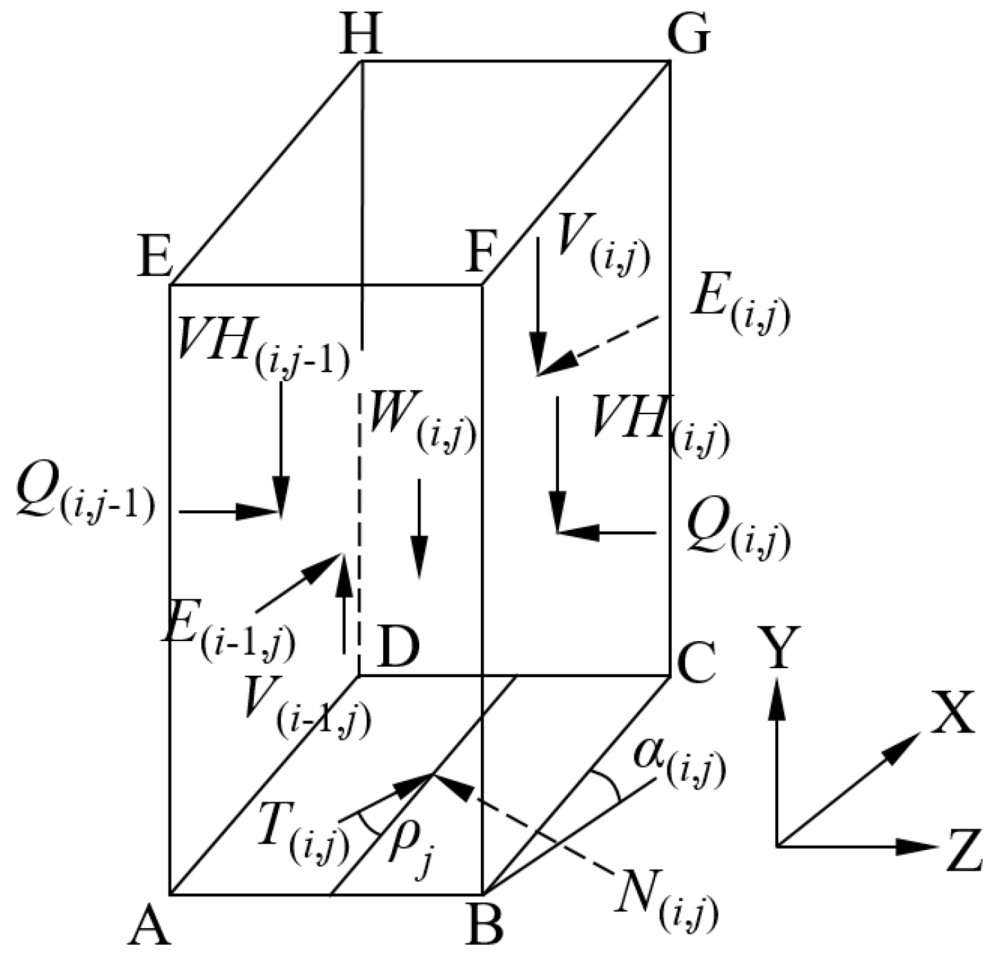
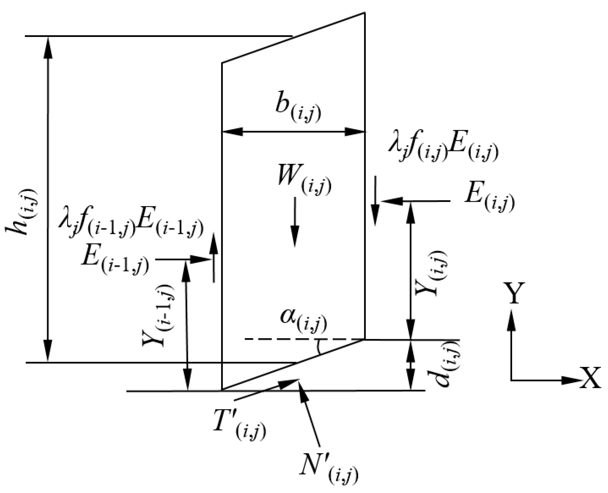
The inter-column shear force $V_{\left(i,j\right)}$ and normal force $E_{\left(i,j\right)}$ exerting on the row face (parallel to $\mathrm{YOZ}$ plane, i.e., face $\mathrm{DCGH}$ in Figure 2) of the typical column labeled by $\left(i,j\right)$ conform to the equation [18] as:

$$V_{\left(i,j\right)}={\mathsf{\lambda }}_j{f}_{\left(i,j\right)}\left(s\right)E_{\left(i,j\right)}$$

(1)

where ${\mathsf{\lambda }}_j$ is the proportional coefficient with the constant value for column group with the same column number $j$ (the subscript indicates the decisive variable on which the value of this coefficient is dependent, the same meaning applies to the definition of following coefficients), and $f_{\left(i,j\right)}\left(s\right)$ is the inter-column force function [29] given by:

$$f_{\left(i,j\right)}\left(s\right)=si{n}^{A_j}\left[B_j\left(s\right)\pi \right]$$

(2)

in which $A_j$ is the shape coefficient for inter-column force function; $B_j\left(s\right)$ is the function characterizing the relative position of this typical column against the column with maximum $x$ coordinate in the column group with the same column number $j$:

$$B_j\left(s\right)=\{\begin{array}{cc}\frac{S_{\left(i,j\right)}}{2s_{fj}}& 0\le S_{\left(i,j\right)}\le s_{fj}\\ \frac{1-2s_{fj}+S_{\left(i,j\right)}}{2\left(1-2s_{fj}\right)}& S_{\left(i,j\right)}\le s_{fj}\le 1\end{array}$$

(3)

where $S_{(i,j)}$ is the normalized x coordinate of the center for the base of the $\left(i,j\right)$ column; $s_{fj}$ is the maximum in the set of $S_{\left(i,j\right)}$ for the column group with the same column number $j$.

(2)

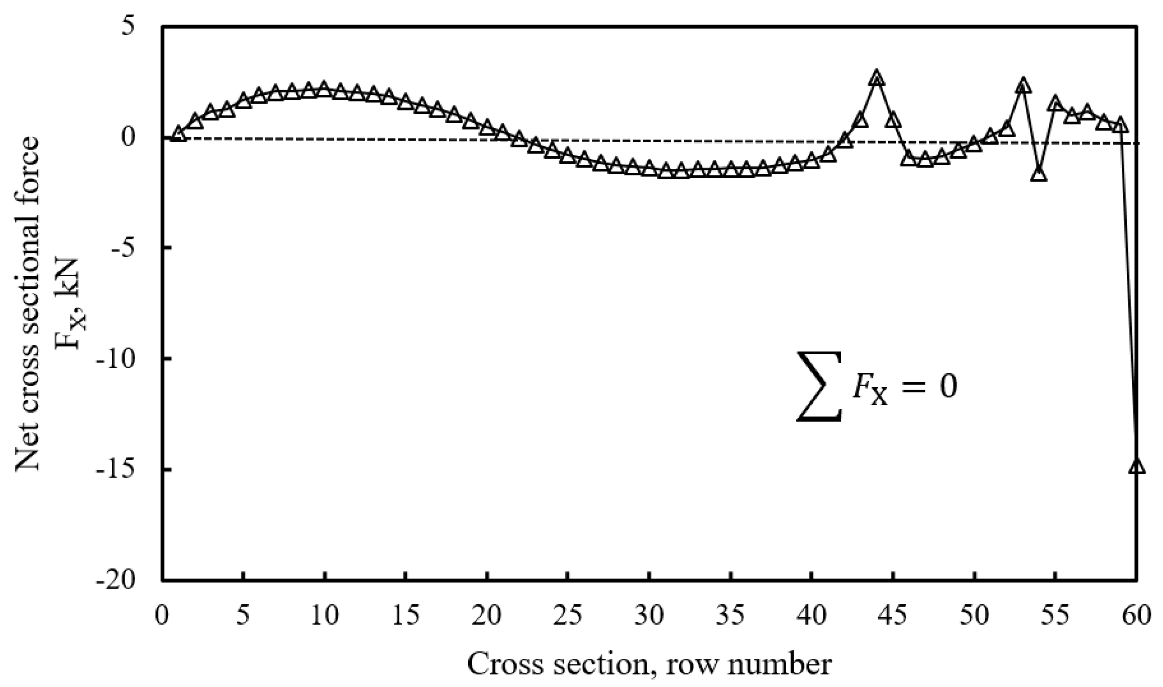
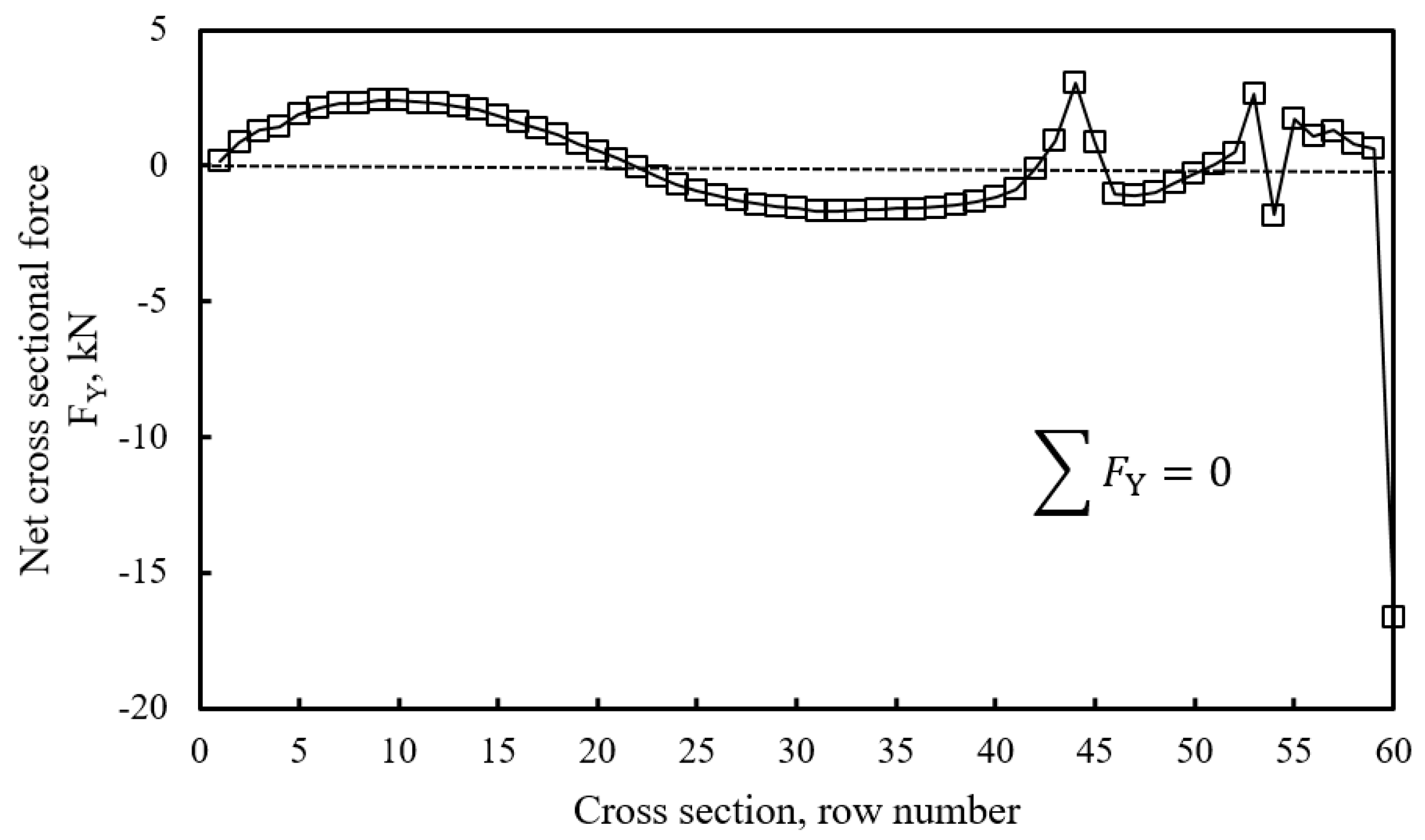
The inter-column normal force $Q_{\left(i,j\right)}$ in the $\mathrm{Z}$ axis direction and inter-column shear force $S{H}_{\left(i,j\right)}$ in the $\mathrm{Y}$ axis direction exerts on the column face (parallel to $\mathrm{XOY}$ plane, i.e., face $\mathrm{BCGF}$ in Figure 2) are neglected in accordance with the assumption in the 2D M-P method. This implies that the force equilibrium for each column is actually enforced in the $Y$ axis direction, referred to as the main sliding direction.

(3)

Shear force $T_{\left(i,j\right)}$ applies to the column base integrating the whole slip surface, with an inclination angle ${\rho }_j$ over the $\mathrm{XOY}$ plane.

As stated earlier, the single subscript $j$ of ${\rho }_j$ indicates no variation for columns with a different row number but in the column group with a constant column number. The variation of ${\rho }_j$ in the direction of axis $\mathrm{Z}$ was presumed to comply with two optional patterns [30].

(a)

${\rho }_j=\mathrm{constant}$, which means the whole sliding mass moves as a rigid body and generates shear force on each column base in a constant direction, as used in [31].

(b)

The magnitude of ${\rho }_j$ increases linearly with the distance from the position of the neutral plane in the direction of axis $\mathrm{Z}$, but with opposite directions indicated by the signs of $z$ coordinates and by different rates adjusted by the value of $\mathsf{\eta }$ on two sides of the neutral plane, as characterized by functions:

$$\begin{array}{cc}{\rho }_j=\mathsf{\kappa }z& \hspace{1em}z\ge 0\end{array}$$

(4a)

$$\begin{array}{cc}{\rho }_j=\mathsf{\eta }\mathsf{\kappa }z& \hspace{1em}z<0\end{array}$$

(4b)

where $z$ indicates the $z$ coordinate of the base center for each column, of which the sign dictates the sign of the sliding direction, defined as a positive direction by the projection in the positive direction of the Z axis; the coefficient $\mathsf{\eta }$ indicates the asymmetrically increasing rate of ${\rho }_j$ on two sides of the neutral plane; and $\mathsf{\kappa }$ is an unknown involved throughout the formulation to be solved. Note that the symmetricity of the slope geometry and the soil properties on two sides of the neutral plane can render the value of $\mathsf{\kappa }$ by zero and the value of $\mathsf{\eta }$ by unit. This means that the sliding mass moves as a rigid body in the direction perpendicular to the rotational axis. With the solution of $\mathsf{\kappa }$ and $\mathsf{\eta }$ obtained, the sliding orientation of each column is determinate, in addition to the shear force distribution on the slip surface for the whole sliding mass.

The normal direction of each column base is characterized by the direction derivatives $n_{X\left(i,j\right)}$, $n_{Y\left(i,j\right)}$ and $n_{Z\left(i,j\right)}$, and the direction of shear force $T_{\left(i,j\right)}$ on each column base by the direction derivatives $m_{X\left(i,j\right)}$, $m_{Y\left(i,j\right)}$ and $m_{Z\left(i,j\right)}$, deduced by the following equations:

$$m_{Z\left(i,j\right)}=sin{\rho }_j$$

(5)

$$\{\begin{array}{c}{m}_{X\left(i,j\right)}^2+m_{Y\left(i,j\right)}^2+m_{Z\left(i,j\right)}^2=1\\ m_{X\left(i,j\right)}{n}_{X\left(i,j\right)}+m_{Y\left(i,j\right)}{n}_{Y\left(i,j\right)}+m_{Z\left(i,j\right)}{n}_{Z\left(i,j\right)}=0\end{array}$$

(6)

Note that the solutions with $m_{X\left(i,j\right)}<0$ should be eliminated due to the physical insignificance of sliding upward against the gravity of the sliding mass.

2.2. Formulation for Solving Factor of Safety in 3DMPM

(1)

The force equilibrium in the $\mathrm{X}$ axis direction for each column gives:

$$n_{X\left(i,j\right)}{N}_{\left(i,j\right)}+E_{\left(i-1,j\right)}+m_{X\left(i,j\right)}{T}_{\left(i,j\right)}-E_{\left(i,j\right)}=0$$

(7)

(2)

The force equilibrium in the $\mathrm{Y}$ axis direction for each column by substituting Equation (1) gives:

$${\mathsf{\lambda }}_j{f}_{\left(i-1,j\right)}{E}_{\left(i-1,j\right)}-W_{\left(i,j\right)}+m_{Y\left(i,j\right)}{T}_{\left(i,j\right)}+n_{Y\left(i,j\right)}{N}_{\left(i,j\right)}-{\mathsf{\lambda }}_j{f}_{\left(i,j\right)}{E}_{\left(i,j\right)}=0$$

(8)

where $N_{\left(i,j\right)}$ denotes the normal force acting at the base center of each column and $W_{\left(i,j\right)}$ denotes the gravity of each column applying at its centroid.

(3)

The forces on the column base in compliance with the Mohr–Coulomb criterion, that the definition of the factor of safety by the mobilized proportion of the shear strength for each column base to maintain the limit equilibrium state is:

$$T_{\left(i,j\right)}=\frac{\left(N_{\left(i,j\right)}-u_{\left(i,j\right)}{A}_{\left(i,j\right)}\right)tan{\phi }_{\left(i,j\right)}}{F_{sj}}+\frac{C_{\left(i,j\right)}{A}_{\left(i,j\right)}}{F_{sj}}$$

(9)

in which $u_{\left(i,j\right)}$ represents the average pore water pressure on each column base, $A_{\left(i,j\right)}$ is the area of each column base, $C_{\left(i,j\right)}$ is the average cohesion on each column base, and $F_{sj}$ denotes the factor of safety for the column group with the same column number $j$.

Substituting Equation (9) into Equations (7) and (8) respectively yields:

$$\begin{array}{c}\left(n_{X\left(i,j\right)}+\frac{m_{X\left(i,j\right)}tan{\phi }_{\left(i,j\right)}}{F_{sj}}\right)N_{\left(i,j\right)}+E_{\left(i-1,j\right)}-E_{\left(i,j\right)}+\frac{m_{X\left(i,j\right)}{C}_{\left(i,j\right)}{A}_{\left(i,j\right)}}{F_{sj}}\\ -\frac{m_{X\left(i,j\right)}tan{\phi }_{\left(i,j\right)}{u}_{\left(i,j\right)}{A}_{\left(i,j\right)}}{F_{sj}}=0\end{array}$$

(10)

$$\begin{array}{c}\left(n_{Y\left(i,j\right)}+\frac{m_{Y\left(i,j\right)}tan{\phi }_{\left(i,j\right)}}{F_{sj}}\right)N_{\left(i,j\right)}+{\mathsf{\lambda }}_j{f}_{\left(i-1,j\right)}{E}_{\left(i-1,j\right)}-{\mathsf{\lambda }}_j{f}_{\left(i,j\right)}{E}_{\left(i,j\right)}\\ +\frac{m_{Y\left(i,j\right)}{C}_{\left(i,j\right)}{A}_{\left(i,j\right)}}{F_{sj}}-\frac{m_{Y\left(i,j\right)}tan{\phi }_{\left(i,j\right)}{u}_{\left(i,j\right)}{A}_{\left(i,j\right)}}{F_{sj}}-W_{\left(i,j\right)}=0\end{array}$$

(11)

Eliminating $N_{\left(i,j\right)}$ by combining Equations (10) and (11) yields:

$${\mathsf{\Phi }}_{\left(i,j\right)}{E}_{\left(i,j\right)}={\mathsf{\Psi }}_{\left(i-1,j\right)}{\mathsf{\Phi }}_{\left(i-1,j\right)}{E}_{\left(i-1,j\right)}-F_{sj}{P}_{\left(i,j\right)}+R_{\left(i,j\right)}$$

(12)

where:

$${\mathsf{\Phi }}_{\left(i,j\right)}=\left( {\mathsf{\lambda }}_j{f}_{\left(i,j\right)}{m}_{X\left(i,j\right)}-m_{Y\left(i,j\right)}\right)tan{\phi }_{\left(i,j\right)}+\left( {\mathsf{\lambda }}_j{f}_{\left(i,j\right)}{n}_{X\left(i,j\right)}-n_{Y\left(i,j\right)}\right)F_{sj}$$

(13)

$${\mathsf{\Phi }}_{\left(i-1,j\right)}=\left( {\mathsf{\lambda }}_j{f}_{\left(i-1,j\right)}{m}_{X\left(i-1,j\right)}-m_{Y\left(i-1,j\right)}\right)tan{\phi }_{\left(i-1,j\right)}+\left( {\mathsf{\lambda }}_j{f}_{\left(i-1,j\right)}{n}_{X\left(i-1,j\right)}-n_{Y\left(i-1,j\right)}\right)F_{sj}$$

(14)

$${\mathsf{\Psi }}_{\left(i-1,j\right)}=\frac{\left( {\mathsf{\lambda }}_j{f}_{\left(i-1,j\right)}{m}_{X\left(i,j\right)}-m_{Y\left(i,j\right)}\right)tan{\phi }_{\left(i,j\right)}+\left( {\mathsf{\lambda }}_j{f}_{\left(i-1,j\right)}{n}_{X\left(i,j\right)}-n_{Y\left(i,j\right)}\right)F_{sj}}{{\mathsf{\Phi }}_{\left(i-1,j\right)}}$$

(15)

$$P_{\left(i,j\right)}=-n_{X\left(i,j\right)}{W}_{\left(i,j\right)}$$

(16)

and:

$$\begin{array}{c}{R}_{\left(i,j\right)}=m_{X\left(i,j\right)}{W}_{\left(i,j\right)}-\left(m_{X\left(i,j\right)}{n}_{Y\left(i,j\right)}-m_{Y\left(i,j\right)}{n}_{X\left(i,j\right)}\right)m_{Y\left(i,j\right)}tan{\phi }_{\left(i,j\right)}{u}_{\left(i,j\right)}{A}_{\left(i,j\right)}\\ +\left(m_{X\left(i,j\right)}{n}_{Y\left(i,j\right)}-m_{Y\left(i,j\right)}{n}_{X\left(i,j\right)}\right)C_{\left(i,j\right)}{A}_{\left(i,j\right)}\end{array}$$

(17)

The natural slope is free of surcharge, which renders the following force boundary conditions:

$$E_{\left(0,j\right)}=0$$

(18a)

$$E_{\left(L,j\right)}=0$$

(18b)

Combining Equations (13)–(17) and (18a,b) derives the factor of safety for the column group with the same column number $j$:

$$F_{sj}=\frac{{{\displaystyle \sum }}_{i=1}^{L-1}{R}_{\left(i,j\right)}{{\displaystyle \prod }}_{k=i}^{L-1}{\mathsf{\Psi }}_{\left(k,j\right)}+R_{\left(L,j\right)}}{{{\displaystyle \sum }}_{i=1}^{L-1}{P}_{\left(i,j\right)}{{\displaystyle \prod }}_{k=i}^{L-1}{\mathsf{\Psi }}_{\left(k,j\right)}+P_{\left(L,j\right)}}$$

(19)

By taking a constant factor of safety $F_{sj}$ for each column group, referred to as the factor of safety $F_{3s}$ for the whole sliding mass:

$$\left({\displaystyle \sum }_{i=1}^{L-1}{P}_{\left(i,j\right)}{\displaystyle \prod }_{k=i}^{L-1}{\mathsf{\Psi }}_{\left(k,j\right)}+P_{\left(L,j\right)}\right)F_{3s}={\displaystyle \sum }_{i=1}^{L-1}{R}_{\left(i,j\right)}{\displaystyle \prod }_{k=i}^{L-1}{\mathsf{\Psi }}_{\left(k,j\right)}+R_{\left(L,j\right)} \left(j=1,2,\cdots ,M\right)$$

(20)

Summation of the $M$ equations in Equation (20) rewrites the factor of safety for the whole sliding mass as:

$$F_{3s}=\frac{{{\displaystyle \sum }}_{j=1}^M\left({{\displaystyle \sum }}_{i=1}^{L-1}{R}_{\left(i,j\right)}{{\displaystyle \prod }}_{k=i}^{L-1}{\mathsf{\Psi }}_{\left(k,j\right)}+R_{\left(L,j\right)}\right)}{{{\displaystyle \sum }}_{j=1}^M\left({{\displaystyle \sum }}_{i=1}^{L-1}{P}_{\left(i,j\right)}{{\displaystyle \prod }}_{k=i}^{L-1}{\mathsf{\Psi }}_{\left(k,j\right)}+P_{\left(L,j\right)}\right)}$$

(21)

(4)

Establishment of the force equilibrium equation in the $\mathrm{Z}$ axis direction for the whole sliding mass:

$${\displaystyle \sum }{n}_{Z\left(i,j\right)}{N}_{\left(i,j\right)}+{\displaystyle \sum }{m}_{Z\left(i,j\right)}{T}_{\left(i,j\right)}=0$$

(22)

Substituting Equation (9) into Equation (22) yields:

$${\displaystyle \sum }\left[\left(N_{\left(i,j\right)}-u_{\left(i,j\right)}{A}_{\left(i,j\right)}\right)tan{\phi }_{\left(i,j\right)}+C_{\left(i,j\right)}{A}_{\left(i,j\right)}\right]m_{Z\left(i,j\right)}-{\displaystyle \sum }{F}_{3s}{n}_{Z\left(i,j\right)}{N}_{\left(i,j\right)}=0$$

(23)

in which $m_{Z\left(i,j\right)}$ can be rewritten by $m_{Zj}$ by the definition of ${\rho }_j$ in Equation (5).

As $M\times L$ columns were meshed out, Equation (23) can be rewritten by:

$${\displaystyle \sum }_{j=1}^M m_{Zj}{\displaystyle \sum }_{i=1}^L\left[\left(N_{\left(i,j\right)}-u_{\left(i,j\right)}{A}_{\left(i,j\right)}\right)tan{\phi }_{\left(i,j\right)}+C_{\left(i,j\right)}{A}_{\left(i,j\right)}\right]-{\displaystyle \sum }_{j=1}^M{F}_{3s}{\displaystyle \sum }_{i=1}^L{n}_{Z\left(i,j\right)}{N}_{\left(i,j\right)}=0$$

(24)

(a)

If constant ${\rho }_j$ for each column is assumed, summation of Equation (24) for all columns in column group with number $j$ gives:

$$m_{Z\left(i,j\right)}=m_{Zj}=m_Z=\frac{-F_{3s}{{\displaystyle \sum }}_{j=1}^M{{\displaystyle \sum }}_{i=1}^L{n}_{Z\left(i,j\right)}{N}_{\left(i,j\right)}}{{{\displaystyle \sum }}_{j=1}^M{{\displaystyle \sum }}_{i=1}^L\left[\left(N_{\left(i,j\right)}-u_{\left(i,j\right)}{A}_{\left(i,j\right)}\right)tan{\phi }_{\left(i,j\right)}+C_{\left(i,j\right)}{A}_{\left(i,j\right)}\right]}$$

(25)

$${\rho }_j={sin}^{-1}{m}_Z$$

(26)

in which $m_Z$ denotes the constant direction derivative in the $\mathrm{Z}$ axis for the whole sliding mass.

(b)

Columns with centroid coordinate $\mathrm{Z}\ge 0$ (denoted by $Z_{Rj}$) in the column group with number j were labeled by row number in the range $\left[{\mathrm{M}}_1,\cdots ,\mathrm{M}\right]$; thus Equation (24) can be rewritten as:

$$m_{Zj}=\frac{-F_{3s}{{\displaystyle \sum }}_{i=1}^L{n}_{Z\left(i,j\right)}{N}_{\left(i,j\right)}}{{{\displaystyle \sum }}_{i=1}^L\left[\left(N_{\left(i,j\right)}-u_{\left(i,j\right)}{A}_{\left(i,j\right)}\right)tan{\phi }_{\left(i,j\right)}+C_{\left(i,j\right)}{A}_{\left(i,j\right)}\right]}$$

(27)

Combining Equations (4a) and (27) yields:

$$\mathsf{\kappa }{Z}_{Rj}={sin}^{-1}{m}_{Zj}={sin}^{-1}\frac{-F_{3s}{\displaystyle {\sum }_{i=1}^L{n}_{Z\left(i,j\right)}{N}_{\left(i,j\right)}}}{{\displaystyle {\sum }_{i=1}^L\left[\left(N_{\left(i,j\right)}-u_{\left(i,j\right)}{A}_{\left(i,j\right)}\right)tan{\phi }_{\left(i,j\right)}+C_{\left(i,j\right)}{A}_{\left(i,j\right)}\right]}}$$

(28)

The summation of Equation (28) for $\mathrm{M}-M_1+1$ columns with positive $Z_{Rj}$ coordinates yields:

$$\mathsf{\kappa }=\frac{{{\displaystyle \sum }}_{j=M_1}^M{sin}^{-1}\frac{-F_{3s}{{\displaystyle \sum }}_{i=1}^L{n}_{Z\left(i,j\right)}{N}_{\left(i,j\right)}}{{{\displaystyle \sum }}_{i=1}^L\left[\left(N_{\left(i,j\right)}-u_{\left(i,j\right)}{A}_{\left(i,j\right)}\right)tan{\phi }_{\left(i,j\right)}+C_{\left(i,j\right)}{A}_{\left(i,j\right)}\right]}}{{{\displaystyle \sum }}_{j=M_1}^M{Z}_{Rj}}$$

(29)

(c)

Columns with centroid coordinate $\mathrm{Z}<0$ denoted by $Z_{Lj}$ in the column group with column number $j$ were labeled by row number from 1 through $M_1$; thus, the procedure of deriving value of $\mathsf{\kappa }$ was repeated to obtain the value of $\mathsf{\eta }$:

$$\mathsf{\eta }=\frac{{{\displaystyle \sum }}_{j=1}^{M_1}{sin}^{-1}\frac{-F_{3s}{{\displaystyle \sum }}_{i=1}^L{n}_{Z\left(i,j\right)}{N}_{\left(i,j\right)}}{{{\displaystyle \sum }}_{i=1}^L\left[\left(N_{\left(i,j\right)}-u_{\left(i,j\right)}{A}_{\left(i,j\right)}\right)tan{\phi }_{\left(i,j\right)}+C_{\left(i,j\right)}{A}_{\left(i,j\right)}\right]}}{\mathsf{\kappa }{{\displaystyle \sum }}_{j=1}^{M_1}{Z}_{Rj}}$$

(30)

The value of ${\rho }_j$ and the direction derivatives, i.e., $m_{X\left(i,j\right)}$, $m_{Y\left(i,j\right)}$ and $m_{Z\left(i,j\right)}$ of shear force $T_{\left(i,j\right)}$ for each column can be solved in Equations (5) and (6).

As depicted in Figure 3, the average height of each column is denoted by $h_{\left(i,j\right)}$, the base of column $\left(i,j\right)$ is measured by projective length $d_{\left(i,j\right)}$ in the $\mathrm{Y}$ axis direction and $b_{\left(i,j\right)}$ in the X axis direction, respectively.

The moment equilibrium equation about the axis going through the base center and parallel to Z axis can be established as:

$$E_{\left(i,j\right)}\left(Y_{\left(i,j\right)}+\frac{d_{\left(i,j\right)}}{2}\right)=E_{\left(i-1,j\right)}\left(Y_{\left(i-1,j\right)}-\frac{d_{\left(i,j\right)}}{2}\right)+{\mathsf{\lambda }}_j\left(f_{\left(i,j\right)}{E}_{\left(i,j\right)}+f_{\left(i-1,j\right)}{E}_{\left(i-1,j\right)}\right)\frac{b_{\left(i,j\right)}}{2}$$

(31)

in which $Y_{\left(i,j\right)}$ represents the application height of $E_{\left(i,j\right)}$ started from the base side of the application face for each column.

Substituting the definition of moment by $E_{\left(i,j\right)}$ as ${M^{\prime }}_{\left(i,j\right)}=E_{\left(i,j\right)}{Y}_{\left(i,j\right)}$ into Equation (31) yields:

$${M^{\prime }}_{\left(i,j\right)}={M^{\prime }}_{\left(i-1,j\right)}+{\mathsf{\lambda }}_j\left(f_{\left(i,j\right)}{E}_{\left(i,j\right)}+f_{\left(i-1,j\right)}{E}_{\left(i-1,j\right)}\right)\frac{b_{\left(i,j\right)}}{2}-\left(E_{\left(i,j\right)}+E_{\left(i-1,j\right)}\right)\frac{d_{\left(i,j\right)}}{2}$$

(32)

Summation of Equation (32) by adopting moment boundary conditions of ${M^{\prime }}_{\left(0,j\right)}=0$ and ${M^{\prime }}_{\left(L,j\right)}=0$ gives:

$$\mathsf{\eta } {\mathsf{\lambda }}_j{\displaystyle \sum }_{i=1}^L{b}_{\left(i,j\right)}\left(f_{\left(i,j\right)}{E}_{\left(i,j\right)}+f_{\left(i-1,j\right)}{E}_{\left(i-1,j\right)}\right)={\displaystyle \sum }_{i=1}^L{d}_{\left(i,j\right)}\left(E_{\left(i,j\right)}+E_{\left(i-1,j\right)}\right)$$

(33)

Equation (33) can be simplified by giving identical ${\mathsf{\lambda }}_j$, denoted by $\mathsf{\lambda }$ for all columns in column group with column number $j$ but different row numbers, as suggested in [5]:

$$\mathsf{\lambda }\left({\displaystyle \sum }_{i=1}^L{b}_{\left(i,j\right)}\left(f_{\left(i,j\right)}{E}_{\left(i,j\right)}+f_{\left(i-1,j\right)}{E}_{\left(i-1,j\right)}\right)\right)={\displaystyle \sum }_{i=1}^L{d}_{\left(i,j\right)}\left(E_{\left(i,j\right)}+E_{\left(i-1,j\right)}\right) \left(j=1,2,\cdots ,M\right)$$

(34)

Summation of $M$ equations in Equation (34) yields:

$$\mathsf{\lambda }=\frac{{{\displaystyle \sum }}_{j=1}^M{{\displaystyle \sum }}_{i=1}^L{d}_{\left(i,j\right)}\left(E_{\left(i,j\right)}+E_{\left(i-1,j\right)}\right)}{{{\displaystyle \sum }}_{j=1}^M{{\displaystyle \sum }}_{i=1}^L{b}_{\left(i,j\right)}\left(f_{\left(i,j\right)}{E}_{\left(i,j\right)}+f_{\left(i-1,j\right)}{E}_{\left(i-1,j\right)}\right)}$$

(35)

The values of $F_{3s}$, $\mathsf{\lambda }$ and ${\rho }_j$ can be solved by combining Equations (21), (25) and (26) or Equations (27)–(30) and (35).

2.3. The Programming Implementation of 3DMPM

Since the above formulation is featured by recursion equations, the computation is readily implemented by coding in the MATLAB environment with the iteration technique applied to achieve convergence. The specific programming flowchart is summarized in steps as given below.

(1)

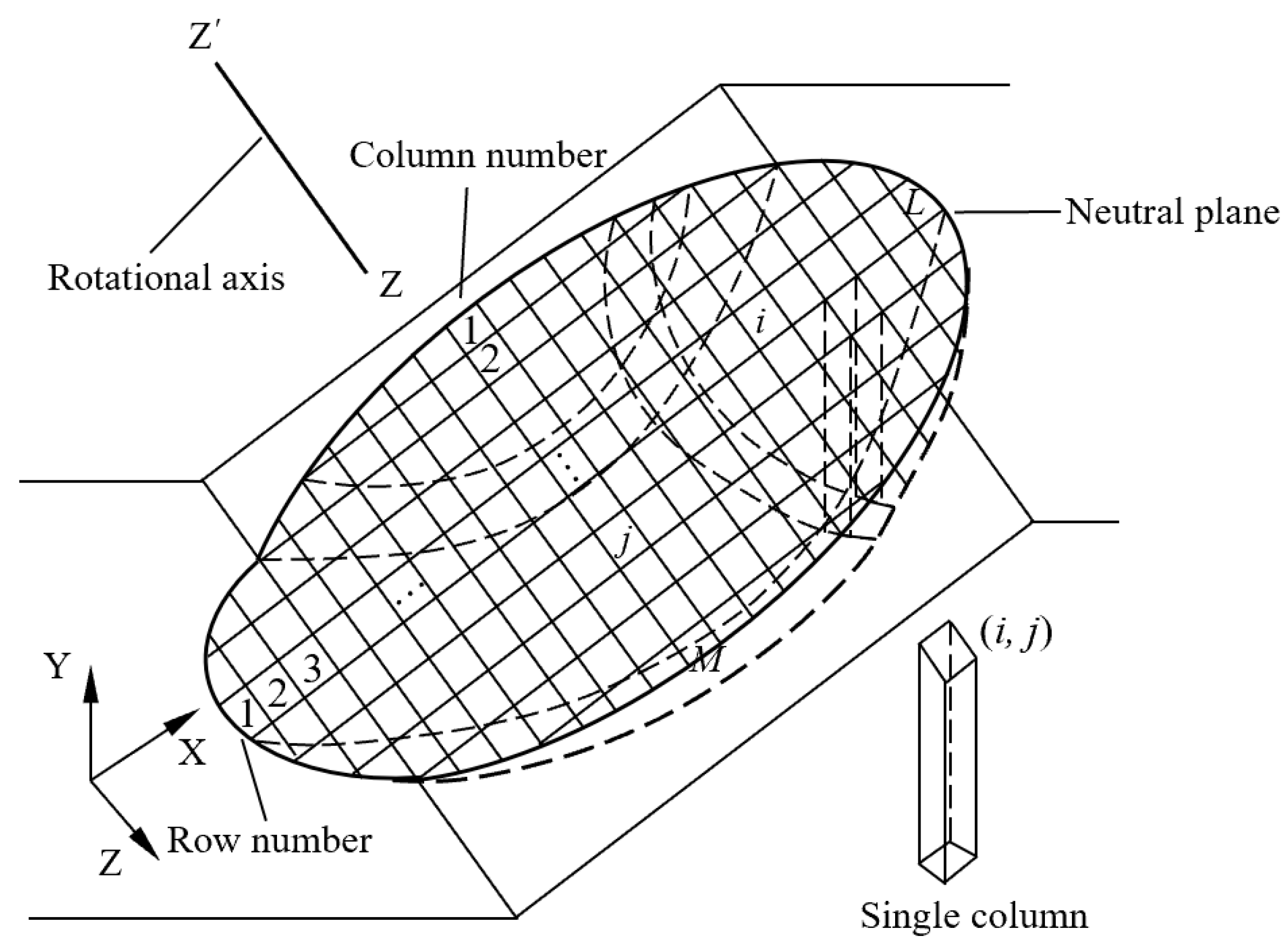
Establish the Cartesian coordinate system upon the sliding mass by aligning the Z axis with the rotational axis, the $\mathrm{XOY}$ plane with the neutral plane with the largest cross-section area, and the origin set at the toe of the neutral plane.

(2)

Mesh the sliding mass into $M\times L$ element columns by the prescribed grid density on the slip surface, label each column by row number along the X axis and column number along the $\mathrm{Z}$ axis illustrated in Figure 1.

(3)

Prescribe the soils’ properties, including unit weight and shear strength parameters, and pore water pressure distribution, to each column according to the information by geological survey.

(4)

Prescribe the initial estimate of unknowns $F_{3s0}$, ${\mathsf{\lambda }}_0$ and ${\rho }_0$ for constant pattern (or ${\mathsf{\kappa }}_0$ and ${\mathsf{\eta }}_0$ for linear pattern) by rough evaluation of the geometric and mechanic characteristics of the object sliding mass.

(5)

Gravity $W_{\left(i,j\right)}$ and gravity-related intermediate forces $P_{\left(i,j\right)}$ and $R_{\left(i,j\right)}$ can be calculated in Equations (16) and (17) for each column.

(6)

Angle-related intermediate variables ${\mathsf{\Phi }}_{\left(i,j\right)}$ and ${\mathsf{\Psi }}_{\left(i-1,j\right)}$ can be obtained by substituting $F_{3s0}$ and ${\mathsf{\lambda }}_0$ into Equations (13)–(15) with direction derivatives solved in Equations (5) and (6) by ${\rho }_0$ or ${\mathsf{\kappa }}_0$ and ${\mathsf{\eta }}_0$.

(7)

The value of $F_{3s}$ evolved by substitution of ${\mathsf{\Phi }}_{\left(i,j\right)}$ and ${\mathsf{\Psi }}_{\left(i-1,j\right)}$ into Equation (21).

(8)

Solve ${\mathrm{E}}_{\left(\mathrm{i},\mathrm{j}\right)}$ in Equation (12) by the updated ${\mathrm{F}}_{3\mathrm{s}}$ and the precedent ${\mathsf{\Phi }}_{\left(i,j\right)}$ and ${\mathsf{\Psi }}_{\left(i-1,j\right)}$.

(9)

Update the value of $\mathsf{\lambda }$ by substituting $E_{\left(i,j\right)}$ into Equation (35).

(10)

Solve $N_{\left(i,j\right)}$ and $T_{\left(i,j\right)}$ by using $E_{\left(i,j\right)}$, $F_{3s}$, ${\mathsf{\Phi }}_{\left(i,j\right)}$ and ${\mathsf{\Psi }}_{\left(i-1,j\right)}$ in Equations (9) and (10).

(11)

Update the value of $\rho$ or $\mathsf{\kappa }$ and $\mathsf{\eta }$ by calculation of Equations (25) and (26) or Equations (27)–(30) with $N_{\left(i,j\right)}$ and $F_{3s}$.

(12)

The initial values of $F_{3s0}$, ${\mathsf{\lambda }}_0$, ${\rho }_0$ or ${\mathsf{\kappa }}_0$ and ${\mathsf{\eta }}_0$ are updated by the above computed results.

(13)

The evolution of prescribed unknowns continues by repeating step (4) through step (12) until the termination criterion are achieved, which were defined by $\left|F_{3s0}-F_{3s}\right|\le {\epsilon }_1$, $\left|{\mathsf{\lambda }}_0-\mathsf{\lambda }\right|\le {\epsilon }_2$, $\left|{\rho }_0-\rho \right|\le {\epsilon }_3$ or $\left|{\left({\mathsf{\kappa }}_0-\mathsf{\kappa }\right)}^2+{\left({\mathsf{\eta }}_0-\mathsf{\eta }\right)}^2\right|\le {\epsilon }_3^2$, where ${\epsilon }_1$, ${\epsilon }_2$ and ${\epsilon }_3$ denote the tolerance prescribed for unknowns.

(14)

Output the solution of $F_{3s}$, $\mathsf{\lambda }$, $\rho$ or $\mathsf{\kappa }$ and $\mathsf{\eta }$.

Note that the computational efficiency for the above program is remarkable. The convergence can be achieved with a few iterations even for a sliding mass with complex geometry, as demonstrated in the later example case. This trait justifies the attempt to apply this extension technique to sampling for slope reliability analysis provided its accuracy and effectiveness in slope stability evaluation is examined, as presented below.

3. Examination of 3DMPM by Reported Example Cases

The application of this 3D extension technique was examined during a practical landslide with irregular geometry reported by Chen et al. [32] and a hypothetic slope with spherical slip surface used by Cheng and Yip [31]. The former example demonstrates the capability of analyzing complex slopes, whereas the latter example provides externally verifiable evidence for the accuracy of the calculated results by this 3DMPM.

3.1. Power Plant Slope of the Tianshengqiao II Project

This slope example originated from an excavation having a height of 170 m at a hydro-power plant construction in China in the late 1980s. The landslide moved by 7.2 mm per day, which means the slip surface had been fully formed. Site investigation by boreholes and observation on uncovered failure soils identified the slip surface by the clay seam, which featured as the weak layer in the rock slope. The slope geometry, including the slope surface and the slip surface, was delivered by nine cross-sections parallel to the neutral plane with coordinates of key nodes in the grid given. It should be noted that the phreatic line in each cross-section marked the ground water level inside the sliding mass but with an absence of coordinate information. The restoration of this sliding mass was completed by the graphic data acquisition tool and the meshing interpolation functions in MATLAB, as demonstrated in Figure 4. The geometric characteristics of the real slope with reported grid density of 25–30 m was reserved by a refined grid density of 5 m as depicted. The reported geotechnical properties for the clay seam and sliding mass were adopted consistently, as shown in Figure 4.

The factor of safety solved for this example case by 3DMPM is 0.9403, which is slightly smaller than the calculated result of 0.945 by Chen’s technique [32]. Eight iterations were required to achieve the convergence and the values of unknowns $F_{3s}$, $\mathsf{\lambda }$, $\rho$ or $\mathsf{\kappa }$ and $\mathsf{\eta }$ were updated accordingly, as given in

Table 1. Iteration process for solving unknowns in the formulation.

Iteration Count	Unknowns	${\mathit{F}}_{3\mathit{s}}$	$\mathsf{\lambda }$	$\mathsf{\kappa }$	$\mathsf{\eta }$
0	Initial value	1	0.1	0.5	1
1	Updated value	0.92904658	0.343899892	0.002694623	1.760167704
2		0.935328933	0.355620079	0.002003866	2.191196578
3		0.941684448	0.353126985	0.00220214	2.011046151
4		0.939967021	0.353642088	0.002155628	2.049847772
5		0.940380074	0.353515887	0.002166378	2.040912157
6		0.940282089	0.353545864	0.002163924	2.042938779
7		0.940304766	0.353538998	0.002164479	2.042479728
8		0.94029961	0.35354055	0.002164355	2.04258301

. Chen’s technique was implemented based on the upper bound theorem in limit analysis, while the extension of the 2D M-P method inherited from the limit equilibrium analysis was affiliated to the lower bound theorem in limit analysis. The minor discrepancy between the two techniques demonstrates the decent approximation of the actual factor of safety by approaching from opposite sides. The applicability of 3DMPM in analyzing complicated slopes is, in practice, justified by giving effective evaluations in excellent agreement with the reported benchmark.

Interestingly enough, the column with negative $\mathrm{z}$ coordinates tends to move apart from the neutral plane in the orientation double that of the column at the symmetric position, as indicated by the value of $\mathsf{\eta }$ at 2.04. It should be kept in mind that the movement of the sliding mass is an instant condition that is not able to indicate kinematic admissibility or the evolution of slope failure, except for characterizing the direction of the shear force at the column base.

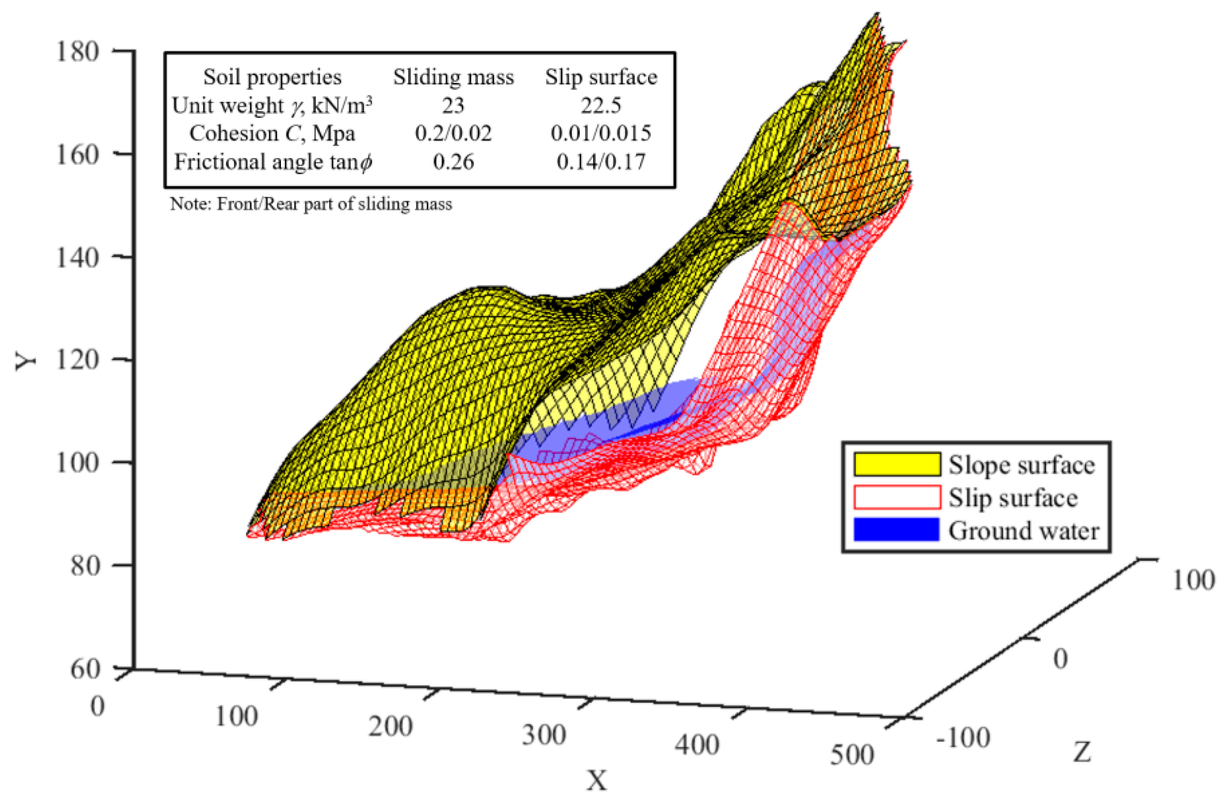
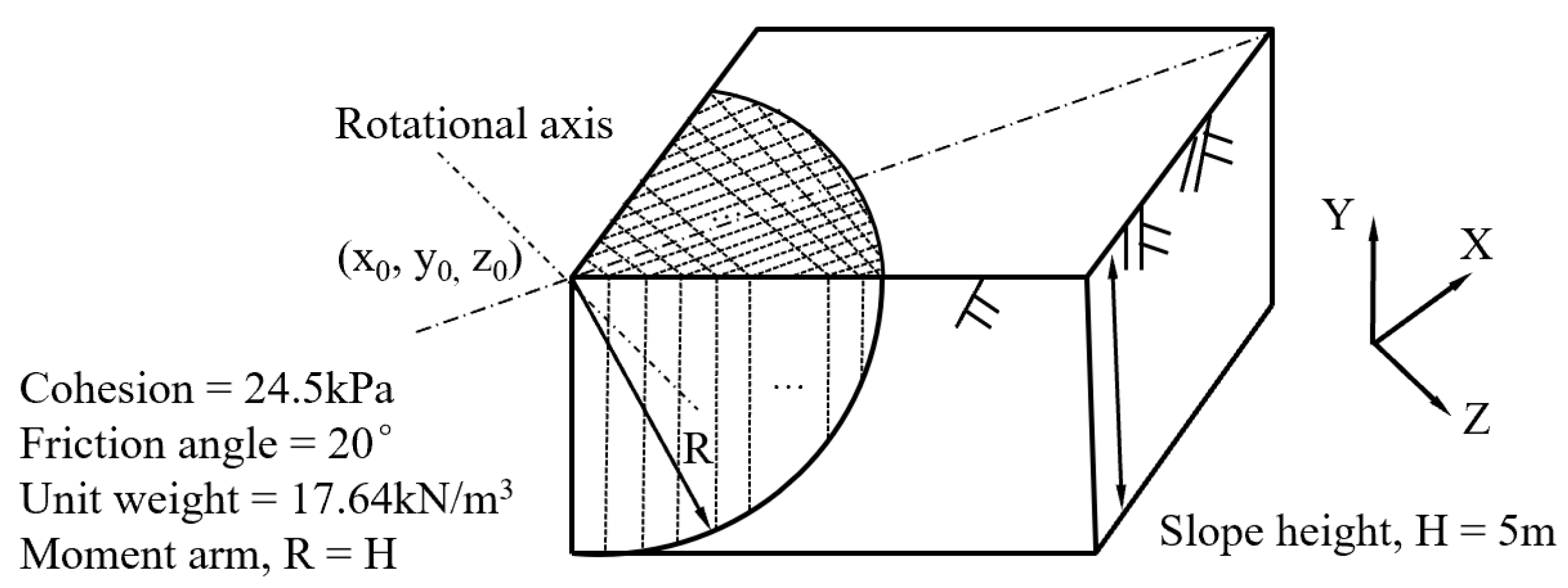
3.2. Hypothetic Slope Example with Spherical Slip Surface

This vertical cup slope was used in an examination of extensions by Huang and Tsai. [8] and Cheng and Yip [31], as seen in Figure 5. The sliding mass is idealized to be a quarter of the sphere with a vertical symmetrical face at the bisection plane. The coordinate system was set by taking the $\mathrm{XOY}$ face (i.e., neutral plane) as the symmetrical face and the $\mathrm{Z}$ axis as its normal direction. The meshing was implemented based on the coordinate system by giving label numbers $M=L=60$ in Figure 1. Note that the complete symmetricity of this example deduces the scenario of $\mathsf{\kappa }=0$ in Equation (4a,b), which means the sliding direction is constantly parallel to the neutral plane for each column, as explained in earlier section.

The factor of safety solved by 3DMPM is close to that by Morgenstern–Price extension in [31], with values of 1.874 and 1.803, respectively. It is stated that all extensions of 2D slice methods are not capable of satisfying cross-sectional force equilibrium due to the high indeterminacy inherent in the formulation [31,33]. The cross-sectional force equilibrium condition for the row face perpendicular to the sliding direction was evaluated in this extension, as shown in Figure 6 and Figure 7. The fluctuation is illustrated around the zero within the amplitude of 5 kN, except at the jump on the last cross-section located at the crest of the sliding mass. This abnormal jump can be ascribed to the consistent meshing method at the crest, which produces several columns at the last cross-section. A refined meshing alternative should be adopted at the crest in order to eliminate this problem but was not implemented in this work. It is expected that the failure of the force equilibrium at each cross-section would lead to the summation of zero, which indicates the close solution of the force equilibrium for the whole sliding mass.

The two examples demonstrate the capability of this extension for evaluating the stability condition for both the complex slope in practice and the hypothetical slope in examination. It does so by giving an estimate for the factor of safety that is close to that via the other extensions. This applicability in stability analysis justifies the application of 3DMPM to the slope reliability evaluation, as presented in the following sections by incorporating with RSM to obviate the difficulty in solving the performance function induced by the implicit formulation, as stated in the introduction.

4. Reliability Evaluation on Hypothetic Slope Example by 3DMPM and RSM

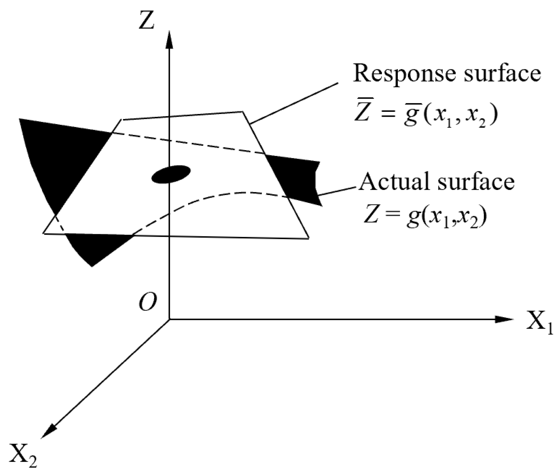
4.1. Fundamentals of the Response Surface Method

In the conventional reliability analysis of structures, the core idea of RSM is the establishment of the surrogate function with explicit expression. It aims at fitting the structural response with the structural model parameters through the completion of random sampling based on numerical computations [33]. This surrogate function denoted by the response surface is initialized and prescribed to replace the actual surface around a certain position of sample space, as depicted in Figure 8 with performance function $\mathrm{Z}=\mathrm{g}\left(x_1,x_2\right)$ and two random variables $x_1$ and $x_2$. Note that it is not necessary to find a response surface function that fits well with the actual surface in the entire sample space, on the grounds that the purpose of reliability analysis is to compute the checking points and corresponding reliability indices [25]. The implicitness inherent in the actual performance function would be eliminated by the response surface in the explicit form, with the fitting capacity required only on the small region adjacent to checking points. The induced coefficients characterizing the response surface are solved by interpolation of the numerical random samples. With respect to reliability evaluation on an example case in engineering practice with $N_r$ random variables denoted by $X=\left(x_1,x_2,\dots ,x_{N_r}\right)$, a feasible response surface $\overline{Z}=\overline{g}\left(X\right)$ can be expressed by a quadratic polynomial without crossing terms, seen as:

$$\overline{Z}=\overline{g}\left(X\right)=a+{\displaystyle \sum }_{i=1}^{N_r}{b}_i{x}_i+{\displaystyle \sum }_{i=1}^{N_r}{c}_i{x}_i^2$$

(36)

where $a$, $b_i$ and $c_i$ $\left(i=1,2,\dots ,N_r\right)$ are undetermined coefficients that can be solved by $2N_r+1$ interpolations on samples prior to the response surface being finalized.

4.2. Establishment of Response Surface Model Based on 3DMPM

4.2.1. Determination of Random Variables

Earth slope stability is dominated by a slope geometry that is certain in a specific case and soil properties possessing large uncertainties. Shear strength parameters such as cohesion $C$ and friction angle $\mathsf{\varphi }$ were generally adopted to characterize the random variation by being taken as random variables in slope reliability evaluation [20], and were inherited in this work.

4.2.2. Establishment of Performance Function

The factor of safety in 3DMPM was not solvable by explicit expression in terms of $C$ and $\mathsf{\varphi }$ as suggested in Equation (21). Based on the fundamental of RSM, the implicit function was approximated by a quadratic function with random variables by shear properties for each soil layer:

$$F_{3S}\approx a+{\displaystyle \sum }_{i=1}^{N_r}{b}_i{x}_i+{\displaystyle \sum }_{i=1}^{N_r}{c}_i{x}_i^2$$

(37)

where $x_i$ represent $C_i$ and ${\mathsf{\varphi }}_i$ for different soil layers; for non-laminated slopes, only two random variables were used.

The performance function for slope stability by 3DMPM can be written by:

$$\overline{Z}=\overline{g}\left(X\right)=F_{3S}-1=a-1+{\displaystyle \sum }_{i=1}^{N_r}{b}_i{x}_i+{\displaystyle \sum }_{i=1}^{N_r}{c}_i{x}_i^2$$

(38)

with corresponding limit state equation given by:

$$\overline{g}\left(X\right)=F_{3S}-1=a-1+{\displaystyle \sum }_{i=1}^{N_r}{b}_i{x}_i+{\displaystyle \sum }_{i=1}^{N_r}{c}_i{x}_i^2=0$$

(39)

where $X=\left(x_1,x_2,\dots ,x_{N_r}\right)$ represents the random vector.

4.2.3. Computation of Slope Reliability Index

The program solving $F_{3S}$ in Section 2.3 was employed to complete the sampling in RSM, which was conventionally implemented by numerical simulation. The response surface function can be finalized with undetermined coefficients derived by interpolation on samples. Based on the response surface function, the three-dimensional slope reliability index is solvable using the first-order second-moment technique [22]. The implementation procedure is presented in the following steps.

(1)

Give the mean value ${\mu }_{x_i}$, variation coefficient ${\sigma }_{x_i}$ and correlation coefficient ${\rho }_{x_i}$ for each random variable $x_i$ according to the distribution pattern used in computation, and prescribe an initial minimum reliability index ${\beta }_{\min }$.

(2)

Prescribe the mean value ${\mu }_{x_i}$ of random vector to the initial sample denoted by $X_D^{\left(1\right)}=\left(x_1^{\left(1\right)},x_2^{\left(1\right)},\dots ,x_{N_r}^{\left(1\right)}\right)$.

(3)

Update the $X_D^{\left(1\right)}$ by interpolation close to the sample with $\left(x_1^{\left(1\right)},x_2^{\left(1\right)},\dots ,x_i^{\left(1\right)}\mp f_{rp}{\sigma }_{x_i},\dots ,x_{N_r}^{\left(1\right)}\right)$ and obtain $2N_r+1$ samples, where coefficient $f_{rp}$ is a value in the range of $\left[1,3\right]$.

(4)

Obtain $2N_r+1$ estimates of $\overline{g}\left(X_D^{\left(1\right)}\right)$ by Equation (38) and solve the undetermined coefficients $a$, $b_i$ and $c_i$ $\left(i=1,2,\dots ,N_r\right)$ in the response surface function.

(5)

Solve the checking point $X_D^{*\left(k\right)}$ and reliability index ${\beta }^{\left(k\right)}$ ($k$ indicates the $k^{\mathrm{th}}$ iteration) using the first-order second-moment method.

(6)

Examine the value of $\left|{\beta }^{\left(k\right)}-{\beta }^{\left(k-1\right)}\right|$ by comparing it with the prescribed tolerance; if it is larger than the tolerance, update the $X_D^{\left(k\right)}$ by $X_D^{\left(k+1\right)}=X_D^{\left(k\right)}+\overline{g}\left(X_D^{\left(k\right)}\right)\left(X_D^{*\left(k\right)}-X_D^{\left(k\right)}\right)/\left(\overline{g}\left(X_D^{\left(k\right)}\right)-\overline{g}\left(X_D^{*\left(k\right)}\right)\right)$ and update the response surface approaching the limit state by looping with steps (3)–(5); if the tolerance is achieved, output the failure probability by $P_f=\mathsf{\Phi }\left(-{\beta }^{\left(k\right)}\right)$ and final reliability ${\beta }^{\left(k\right)}$; then, the minimum reliability index ${\beta }_{\min }$ should be evolved in the next loop by ${\beta }^{\left(k\right)}$ if ${\beta }_{\min }>{\beta }^{\left(k\right)}$.

4.3. Application to Hypothetic Example Case

4.3.1. Example Case

The reliability evaluation technique was applied to the hypothetical slope example used in Section 3.2, as shown in Figure 5. Additional statistic properties were prescribed to the cohesion and frictional angle of the hypothetic slope soils, as seen in

Table 2. Statistic properties for slope soils.

Statistic Properties	$\mathbf{Mean}\mathbf{Value}{\mathit{\mu }}_{\mathit{x}}$	$\mathbf{Variation}\mathbf{Coefficient}{\mathit{\sigma }}_{\mathit{x}}$
Cohesion $C$	24.5 kPa	0.15
Friction angle $\mathsf{\varphi }$	20°	0.15

, by referring to available publications associated with slope reliability analysis [20]. The Monte-Carlo technique [34] was employed to calculate the benchmark reliability and this presented technique’s accuracy and efficiency was demonstrated by comparison as shown in

Table 3. Comparison with the Monte-Carlo technique.

Establishment of Performance Function	Method Solving Reliability	$\mathbf{Reliability}\mathbf{Index}{\mathit{\beta }}_{3\mathit{D}}$	Error, %	Running Time, Seconds
3DMPM&RSM	First-order second-moment	4.073	0.37	2
3DMPM	Monte-Carlo	4.057	--	16,292

. For simplicity, the example case under computation prescribed independent random variables with a normal probability distribution by the correlation coefficient of zero. On a personal computer with an Intel(R) Core(TM) i5-4210U CPU @ 1.70 GHz 2.40 GHz processor, the time consumption of this presented technique is about one ten-thousandth of that needed in the Monte-Carlo technique, with an error margin of $0.37$ percent. With acceptable engineering precision, the efficiency improvement justifies the priority and the applicability of this presented technique in evaluating three-dimensional slope reliability.

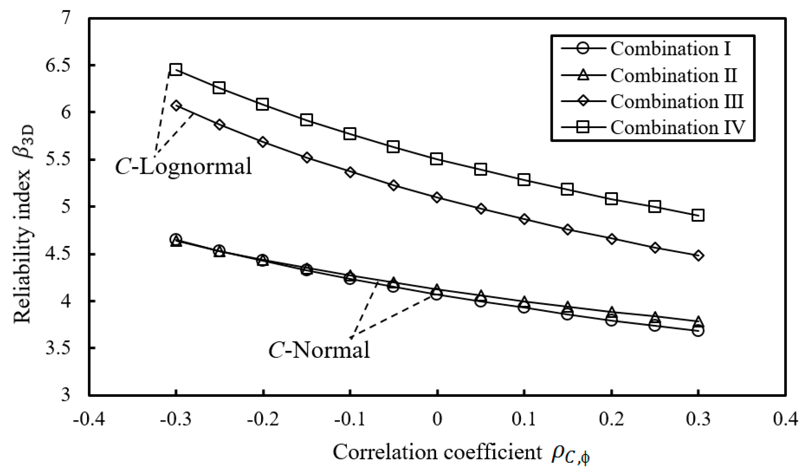
4.3.2. Discussion

It should be noted that the two shear strength parameters are not independent variables in this work, which could manifest different probability distribution patterns. Further, the correlation coefficient between them tends to have a significant impact on the reliability evaluation, as reported in other studies [35,36]. Thus, in order to obtain a wider understanding of the spatial variability of slope soils, the commonly used lognormal distribution and normal distribution were adopted to characterize $C$ and $\mathsf{\varphi }$ in computation, which generated four combinations as shown in

Table 4. Slope reliability with different probability distribution patterns and correlation coefficients.

Combination	Probability Distribution Pattern		$\mathbf{Correlation}\mathbf{Coefficient}{\mathit{\rho }}_{\mathit{C},\mathit{\varphi }}$
	$\mathbf{Cohesion}\mathit{C}$	$\mathbf{Friction}\mathbf{Angle}\mathit{\varphi }$	−0.3	−0.2	−0.1	0	0.1	0.2	0.3
Ⅰ	Normal	Normal	4.645	4.426	4.237	4.073	3.927	3.796	3.677
Ⅱ	Normal	Lognormal	4.635	4.436	4.268	4.122	3.997	3.885	3.785
Ⅲ	Lognormal	Normal	6.075	5.690	5.370	5.099	4.865	4.662	4.482
Ⅳ	Lognormal	Lognormal	6.454	6.080	5.769	5.507	5.280	5.083	4.909

. The correlation coefficient ${\rho }_{C,\mathsf{\varphi }}$ was prescribed from −0.3 through 0.3, bearing in mind the overlap range formed by the values found in other relevant works [22]. The reliability results ${\beta }_{3\mathrm{D}}$ calculated by this technique with respect to each parameter set are also presented in Table 4 and plotted in Figure 9.

The decreasing trend of the reliability index with increasing correlation coefficient is observed for all combinations. Certainly, this indicates the importance of giving a reasonable correlation coefficient between random variables in slope reliability analysis. This influence deserves more attention when the cohesion conforms to the lognormal probability distribution, which can be revealed by the larger decreasing rate in profiles labeled by C-Lognormal in Figure 9. Furthermore, of continued interest, is the insensitivity of this trend relationally to the probability distribution of the friction angle, as demonstrated by the similar slope variation of the two profiles for combinations featured by C-Lognormal and C-Normal. This insensitivity in the switch between ϕ-Lognormal and ϕ-Normal is manifested not only in the varying trend, but also in the value of the reliability index for the cases of C-Normal.

The difference ratio of the reliability index induced by switching exclusively the probability distribution of the cohesion or the friction angle is illustrated by cross-analysis in Figure 10. Note that the label close to the plotting indicates the consistent variable; for example, ϕ-Normal denotes the difference ratio induced by the switch between C-Lognormal and C-Normal. The larger difference ratio in the four cases suggests that the presence of this probability distribution tends to make the calculated reliability results more sensitive to the selection of the correlation coefficient, and the selection of the probability distribution pattern of other random variables. In other words, the stability degree of the calculated results for slope reliability can be characterized by this plotting. The dominant priority in this reliability evaluation can be ranked by C > ϕ and Normal > Lognormal, which explains the highest turbulence in the case of ϕ-Lognormal and the lowest in the case of C-Normal. It is worth mentioning that the relative priority formed between the cohesion and the friction angle is expected to be mitigated with the increasing correlation coefficient, as indicated by the opposite trends in the profiles for C-distribution and ϕ-distribution.

Furthermore, final remarks regarding slope reliability analysis can be made: (a) the increasing correlation coefficient between selected random variables would lead to the decrease in the reliability index by an extent depending on the variables’ probability distribution pattern; (b) the cohesion plays a larger role than the friction angle in the influence on the reliability induced by its probability distribution pattern; and (c) the normal distribution of the random variable tends to dominate the stability degree of reliability results more significantly than the lognormal distribution.

5. Conclusions

This work developed a three-dimensional slope reliability evaluation framework by incorporating the extended Morgenstern–Price stability analysis formulations into the response surface method. The applicability and efficiency of the extended stability analysis method and reliability evaluation framework were validated using a complicated landslide from practice and a hypothetical slope example from the literature. Based on the framework, the sensitivity of the reliability index on probabilistic statistic parameters was examined. The concluding remarks of this work are as follows:

• The extended three-dimensional stability analysis method is capable of accounting for the inter-column forces along the main sliding direction and the sliding direction variation on each column, and is applicable to slope cases with highly asymmetric or symmetric slip surfaces.
• The reliability evaluation framework was found to attain better efficiency by incorporating the above stability analysis into the response surface method than that using Monte-Carlo technique.
• The increasing correlation coefficient between the cohesion and the friction angle can reduce the slope reliability index.
• The switch of the probability distribution pattern for the cohesion leads to more significant degradation of the reliability index than that for the friction angle.

The findings obtained in this work may provide insights into the understanding of slope failure or landslides by accounting for soil stochastic effects, and can be used as a reference in the design practice of three-dimensional slope reliability. The impact of statistical parameters of soils on the slope reliability in terms of additional aspects, particularly the time-variant behavior, will be investigated in the future to improve the applicability of the presented reliability evaluation framework.

References

- Duncan, J.M. State of the art: Limit equilibrium and finite-element analysis of slopes. J. Geotech. Eng. 1996, 122, 577–596. [Google Scholar] [CrossRef]
- Liu, J.; Wu, C.; Wu, G.; Wang, X. A novel differential search algorithm and applications for structure design. Appl. Math. Comput. 2015, 268, 246–269. [Google Scholar] [CrossRef]
- Kalatehjari, R.; Ali, N. A review of three-dimensional slope stability analyses based on limit equilibrium method. Electron. J. Geotech. Eng. 2013, 18, 119–134. [Google Scholar]
- Zhang, J.; Li, M.; Ke, L.; Yi, J. Distributions of lateral earth pressure behind rock-socketed circular diaphragm walls considering radial deflection. Comput. Geotech. 2022, 143, 104604. [Google Scholar] [CrossRef]
- Lam, L.; Fredlund, D. A general limit equilibrium model for three-dimensional slope stability analysis. Can. Geotech. J. 1993, 30, 905–919. [Google Scholar] [CrossRef]
- Dong, H.; Zhao, B.; Deng, Y. Instability phenomenon associated with two typical high speed railway vehicles. Int. J. Non-Lin. Mech. 2018, 105, 130–145. [Google Scholar] [CrossRef]
- Hungr, O.; Salgado, F.; Byrne, P. Evaluation of a three-dimensional method of slope stability analysis. Can. Geotech. J. 1989, 26, 679–686. [Google Scholar] [CrossRef]
- Huang, C.-C.; Tsai, C.-C. New method for 3D and asymmetrical slope stability analysis. J. Geotech. Geoenviron. Eng. 2000, 126, 917–927. [Google Scholar] [CrossRef]
- Hovland, H.J. Three-dimensional slope stability analysis method. J. Geotech. Eng. Div. 1977, 103, 971–986. [Google Scholar] [CrossRef]
- Lu, K.; Wang, L.; Yang, Y.; Zhou, G. Three-dimensional method for slope stability with the curvilinear route of the main sliding. Bull. Eng. Geol. Environ. 2022, 81, 67. [Google Scholar] [CrossRef]
- Michalowski, R. Three-dimensional analysis of locally loaded slopes. Géotechnique 1989, 39, 27–38. [Google Scholar] [CrossRef]
- Chen, Z.; Wang, X.; Haberfield, C.; Yin, J.; Wang, Y. A three-dimensional slope stability analysis method using the upper bound theorem: Part I: Theory and methods. Int. J. Rock Mech. Min. 2001, 38, 369–378. [Google Scholar] [CrossRef]
- Gao, Y.; Zhang, F.; Lei, G.; Li, D. An extended limit analysis of three-dimensional slope stability. Géotechnique 2013, 63, 518–524. [Google Scholar] [CrossRef]
- Zheng, H. A three-dimensional rigorous method for stability analysis of landslides. Eng. Geol. 2012, 145–146, 30–40. [Google Scholar] [CrossRef]
- Kalatehjari, R.; Arefnia, A.; Rashid, A.; Ali, N.; Hajihassani, M. Determination of three-dimensional shape of failure in soil slopes. Can. Geotech. J. 2015, 52, 1283–1301. [Google Scholar] [CrossRef]
- Fang, Q.; Wang, G.; Yu, F.; Du, J. Analytical algorithm for longitudinal deformation profile of a deep tunnel. J. Rock Mech. Geotech. Eng. 2021, 13, 845–854. [Google Scholar] [CrossRef]
- Morgenstern, N.; Price, V. The analysis of the stability of general slip surfaces. Géotechnique 1965, 15, 79–93. [Google Scholar] [CrossRef]
- Chen, C.; Zhu, J. A three-dimensional slope stability analysis procedure based on Morgenstern-Price method. Chin. J. Rock Mech. Eng. 2010, 29, 1473–1480. [Google Scholar]
- Ling, D.; Qi, S.; Chen, F.; Li, N. A limit equilibrium method based on Morgenstern-Price method for 3D slope stability analysis. Chin. J. Rock Mech. Eng. 2013, 32, 107–116. [Google Scholar]
- Xiao, T.; Li, D.; Cao, Z.; Au, S.; Phoon, K. Three-dimensional slope reliability and risk assessment using auxiliary random finite element method. Comput. Geotech. 2016, 79, 146–158. [Google Scholar] [CrossRef] [Green Version]
- Song, L.; Xu, B.; Kong, X.; Zou, D.; Pang, R.; Yu, X.; Zhang, Z. Three-dimensional slope dynamic stability reliability assessment based on the probability density evolution method. Soil Dyn. Earthq. Eng. 2019, 120, 360–368. [Google Scholar] [CrossRef]
- Cho, S. Effects of spatial variability of soil properties on slope stability. Eng. Geol. 2007, 92, 97–109. [Google Scholar] [CrossRef]
- Low, B.; Gilbert, R.; Wright, S. Slope reliability analysis using generalized method of slices. J. Geotech. Geoenviron. Eng. 1998, 124, 350–362. [Google Scholar] [CrossRef]
- Wong, F. Slope reliability and response surface method. J. Geotech. Eng. 1985, 111, 32–53. [Google Scholar] [CrossRef]
- Zhu, B.; Pei, H.; Yang, Q. An intelligent response surface method for analyzing slope reliability based on Gaussian process regression. Int. J. Numer. Methods Eng. 2019, 43, 2431–2448. [Google Scholar] [CrossRef]
- Li, L.; Chu, X. Comparative study on response surfaces for reliability analysis of spatially variable soil slope. China Ocean Eng. 2015, 29, 81–90. [Google Scholar] [CrossRef]
- Li, D.; Zheng, D.; Cao, Z.; Tang, X.; Phoon, K. Response surface methods for slope reliability analysis: Review and comparison. Eng. Geol. 2016, 203, 3–14. [Google Scholar] [CrossRef]
- Chen, C.; Zhu, J.; Gong, X. Calculation method of earth slope reliability based on response surface method and Morgenstern-price procedure. Eng. Mech. 2008, 25, 166–172. [Google Scholar]
- Chen, C. Bionic algorithm and its application to slope and excavation engineering. Chin. J. Rock Mech. Eng. 2001, 22, 1578. [Google Scholar]
- Chen, Z.; Mi, H.; Zhang, F.; Wang, X. A simplified method for 3D slope stability analysis. Can. Geotech. J. 2003, 40, 675–683. [Google Scholar] [CrossRef]
- Cheng, Y.; Yip, C. Three-dimensional asymmetrical slope stability analysis extension of Bishop’s, Janbu’s, and Morgenstern–Price’s techniques. J. Geotech. Geoenviron. Eng. 2007, 133, 1544–1555. [Google Scholar] [CrossRef]
- Chen, Z.; Wang, J.; Wang, Y.; Yin, J.; Haberfield, C. A three-dimensional slope stability analysis method using the upper bound theorem Part II: Numerical approaches, applications and extensions. Int. J. Rock Mech. Min. Sci. 2001, 38, 379–397. [Google Scholar] [CrossRef]
- Chen, F.; Zhong, Y.; Gao, X.; Jin, Z.; Wang, E.; Zhu, F.; Shao, X.; He, X. Non-uniform model of relationship between surface strain and rust expansion force of reinforced concrete. Sci. Rep. 2021, 11, 8741. [Google Scholar] [CrossRef]
- Wang, Y.; Cao, Z.; Au, S. Practical reliability analysis of slope stability by advanced Monte Carlo simulations in a spreadsheet. Can. Geotech. J. 2011, 48, 162–172. [Google Scholar] [CrossRef]
- Jiang, S.; Li, D.; Zhang, L.; Zhou, C. Slope reliability analysis considering spatially variable shear strength parameters using a non-intrusive stochastic finite element method. Eng. Geol. 2014, 168, 120–128. [Google Scholar] [CrossRef]
- Zhu, J.; Chen, C.; Zhao, H. An approach to assess the stability of unsaturated multilayered coastal-embankment slope during rainfall infiltration. J. Mar. Sci. Eng. 2019, 7, 165. [Google Scholar] [CrossRef] [Green Version]