Sound-Based Construction Activity Monitoring with Deep Learning

Abstract

Automated construction monitoring assists site managers in managing safety, schedule, and productivity effectively. Existing research focuses on identifying construction sounds to determine the type of construction activity. However, there are two major limitations: the inability to handle a mixed sound environment in which multiple construction activity sounds occur simultaneously, and the inability to precisely locate the start and end times of each individual construction activity. This research aims to fill this gap through developing an innovative deep learning-based method. The proposed model combines the benefits of Convolutional Neural Network (CNN) for extracting features and Recurrent Neural Network (RNN) for leveraging contextual information to handle construction environments with polyphony and noise. In addition, the dual threshold output permits exact identification of the start and finish timings of individual construction activities. Before training and testing with construction sounds collected from a modular construction factory, the model has been pre-trained with publicly available general sound event data. All of the innovative designs have been confirmed by an ablation study, and two extended experiments were also performed to verify the versatility of the present model in additional construction environments or activities. This model has great potential to be used for autonomous monitoring of construction activities.

1. Introduction

The monitoring of construction is considered to be one of the most important parts of successful project management, which can effectively avoid construction accidents and reduce project duration. The traditional process tracking methods need to be mainly completed by on-site personnel, and this tends to be time-consuming, labor-intensive, and error-prone [1,2]. With affordable sensors applied on construction sites, the construction manager is ready to embrace an automated construction monitoring future [3]. Different automatic data acquisition techniques have been widely explored in construction monitoring tasks, such as computer vision [4,5,6], motion detection [7,8,9], remote sensing techniques [10], and close-range detection [11]. Lately, researchers have reported that sound can be a pervasive and critical source of construction information both on and off-site [12,13].

Automated construction monitoring can be divided into three sublevels, namely identification of current construction activities, tracking of ongoing construction activities, and performance monitoring of completed work [14]. Due to the obvious temporal properties of sound, acoustic techniques are especially well-suited for tracking ongoing construction activities. Compared to vision-based approaches, sound-based methods are not impacted by observation blindness or situations such as light fluctuations and sight obstruction [5]. Sense-based methods at construction sites are often employed to determine the motions of construction machines or personnel, necessitating extra semantic information to comprehend the activity level [3]. In contrast to sense-based methods, sound-based methods can immediately detect activity-level information without the need to filter information at lower levels of detail. As a result, sound-based methods are well suited for tracking the status and duration of resource construction activities, and they have been used on construction sites for schedule management [15], productivity analysis [16], safety management [17], and other applications. Sound is envisaged to contribute to the construction phase’s digital twin [18].

Similarly to machine vision, computer audition is a study field that allows algorithmic audio understanding [19]. Previous research for acoustic analysis of construction activities includes figuring out the type of single activity carried out by a worker [13], the type of single activity performed by construction equipment [20,21], whether a single piece of construction equipment is running or not [12], and the type and model of a single piece of construction equipment [22]. The great majority of the research performed has focused on the identification of distinct single construction activities, based on the premise that only one sort of sound is active at any given moment. Recent study has investigated situations with mixed construction sounds, but this work is still susceptible to certain limitations, such as the assumption that two kinds of construction noises always occur concurrently [23]. Construction sites are polyphonic settings with noise disruptions, since many construction workers or construction machines often operate concurrently [24]. To address these challenges, algorithms with strong detecting capabilities and resilience should be developed further.

In this study, a CRNN (Convolutional Recurrent Neural Network) model consisting of a five-layer CNN and a Bidirectional Gated Recurrent Unit (BiGRU) is constructed, together with a linear output layer and a double threshold. The proposed approach combines the benefits of CNN and RNN, resulting in enhanced sound event detection capabilities and more resilience in complicated sound environments. This developed method can recognize each type of pre-defined sound event and identify the start and end of them, i.e., the correct localization of each single sound event throughout the period [25]. Prior studies of sound classifiers were mainly addressing issues associated with multi-class, namely, only one output class for each input [26]. This research can identify the type and duration of each construction activity separately. Real-world construction settings such as polyphony and noise are likewise no problem for the proposed technique. To train and test the proposed model, we gathered an audio data set of construction sounds in a modular factory. In this CRNN, the combination of CNN and RNN significantly takes advantage of both the feature extracting ability of CNN and the temporal dependency modeling ability of RNN. In addition, this model has been pretrained using a publicly accessible large-scale sound dataset, which contains most types of common sound events. Benchmark comparisons with previous research demonstrate the evident superiority of the present approach. The ablation study confirmed that the combination of CNN and RNN and the introduction of the pre-training process improved the performance of the model. Extended experiments indicate that the proposed model can also be employed in other construction scenarios or activities, such as refurbishment.

The key findings and novelty of the present approach are as follows:

(1)

Pioneering in real-world practice identifying and monitoring sound events in noisy and coupled situations;

(2)

Succeeding in event classification and temporal localization by determining the start and end of individual events;

(3)

Automating the process in the end-to-end model with direct file input to obtain results without manual processing;

(4)

Requiring a small training sample size from the studied site as a pre-trained model;

(5)

Weak labels needed by using a simple labeling mechanism for annotation training.

2. Review and Knowledge Gap

2.1. Review

DACSE (Detection and Classification of Acoustic Scenes and Events) is the most prestigious workshop in the machine audition research field, and the DCASE 2022 challenge includes tasks of acoustic scene classification, anomalous sound detection, sound event detection and localization, and automated audio captioning [27]. However, only domestic and street scenes are included in the DCASE audio collection that is accessible to the public, which excludes construction scenes. Researchers in the construction industry seek to expand the sound event detection task for the recognition of construction activities on site. The research conducted for this purpose can be divided into traditional machine learning approaches and deep learning approaches, with the primary distinction being whether or not the models use deep neural networks. The two basic components of traditional machine learning approaches are the acoustic feature extraction method and the statistical learning-based model [28]. Deep learning algorithms, on the other hand, employ spectrogram or filterbank outputs as input features and can thus give end-to-end models [29].

In the early stages of constructing sound recognition and monitoring, machine learning methods such as SVM (Support Vector Machines), HMM (Hidden Markov Model), and ELM (Extreme Learning Machine) were intensively investigated. Typically, these techniques depend on manually picked sound features, which are usually produced directly from 2D spectrograms, MFCCs, or Mel-spectrograms. Thomas and Li reported the identification of construction equipment using acoustic data, which is the earliest known work in this field [30]. Cho et al. suggested an HMM model capable of classifying the spectrogram-obtained acoustic features to identify three kinds of construction activities. Besides, they provided a method for displaying the identification results in BIM [31]. Five feature types were collected from the audio using Fourier transform, and a probabilistic model was created to determine the scraper loader’s movement condition. Cheng et al. employed SVM to determine whether four different types of construction machines fell into the major or minor activity categories [32]. In their work, STFT (Short-Time Fourier Transform) was used to transform audio signals into a time-frequency representation, which served as an input. They eventually extended the scope of this investigation and included 11 types of construction machinery [12]. Cao et al. classified excavator construction operations using an Extreme Learning Machine (ELM) and retrieved spectrum dynamic characteristics [33]. Moreover, they designed a cascade classifier that could handle a wide range of sound features, including short frame energy ratio, concentration of spectrum amplitude ratio, truncated energy range, and interval of pulse [34]. Zhang et al. employed a three-state HMM architecture model to classify six different kinds of concreting work [16]. In this research, MFCCs (Mel-scale Frequency Cepstral Coefficients) were used as acoustic characteristics to recognize sounds, and a maximum classification accuracy of 94.3% was also obtained. Rashid and Louis demonstrated that when SVM was used to classify construction activity sounds associated with modular construction, an F1-Score of 97% could be achieved [13]. Akbal and Tuncer reported an SVM-based technique that achieved up to 99.45% accuracy using 256 retrieved acoustic features [21]. Sabillon et al. developed a Bayesian model for the productivity estimation of cyclic construction activities, such as excavation, on construction sites [15]. This model’s input consists of two components, i.e., the SVM as an audio feature classifier that identifies the current activity state, and the Markov chain that predicts the output based on temporal analysis [35]. The Bayesian model will assess the current state of construction based on the outcomes of both inputs.

Traditional machine learning techniques entail first gathering annotated training sets of sounds and then training models using supervised learning [36]. The primary benefit of these methods is the ability to train the model to an acceptable level with limited data samples. However, the accuracy of this strategy is dependent on the quality of the manually selected feature classes, making it difficult to exclude the effect of human design mistakes on model performance [37]. As Rashid and Louis’ study indicated, there was substantial variation in the categorization performance of several sound characteristics associated with construction activities [13]. Moreover, despite the fact that several researchers have tried to apply this family of approaches to the issue of polyphony detection, sophisticated model structures or extra training procedures are necessary [38]. Therefore, traditional machine learning techniques are insufficient for complicated acoustic situations or when a high rate of identification accuracy is required.

Researchers have recently given attention to DBN (Deep Belief Network), CNN (Convolutional Neural Network), and RNN (Recurrent Neural Network) as a result of the development of deep learning technologies. Research in the field of machine audition has revealed the particular benefits of deep learning techniques. Maccagno et al. used CNN to classify the construction environmental sound [39]. In their study, different types and brands of construction vehicles and devices could be recognized. Their study demonstrated the better performance of CNN in classifying construction activities compared to the traditional classifiers such as SVM, KNN (K-Nearest Neighbor), and RF (Random Forest). Lee et al. examined the classification accuracy of 17 classical classification techniques and three deep learning methods such as CNN, RNN, and Deep Belief Network (DBN) for construction activity noises [20]. Moreover, it was found that the best approach achieved a classification accuracy of 93.16%. Scarpiniti et al. demonstrated up to 98% accuracy in categorizing more than 10 different types of construction equipment and device using a DBN [22]. Sherafat et al. developed CNN models for recognizing multiple-equipment activities [23,40]. They used a two-level multi-label sound classification scheme that enables concurrent detection of the device kind and their associated activities.

The emergence of deep learning techniques in the area is attributable to the enhanced performance of deep neural networks and the declining price of computer resources. Despite the advantages claimed in the area of computer audition for integrating CNN and RNN, construction-related sound event detection has not yet been researched. The deep neural network is capable of learning multi-layer representation and abstraction of data [41,42], and DAFs (Deep Audio Features) generated using CNNs outperform conventionally extracted characteristics in terms of accuracy and robustness [43,44,45]. Although individual sound events often show interdependency, the context information amongst them can be used as a valid aid for identification [46]. RNNs excel at utilizing contextual information, and the recurrent mechanism in the hidden layers eliminates the need for smoothing frame-wise decisions [29]. Therefore, SOTA deep network structures, such as CRNN, are required for study in this field.

2.2. Knowledge Gap

While existing studies have shown much progress in recognizing construction activities, there are still several limits to their applicability in the real world. Challenges arise from three primary aspects, i.e., (1) complex overlapping sound sources and strongly mingled ambient noise in construction sites; (2) failure of existing methods to localize the start and end time of sound events; and (3) lack of versatility and adaptability of existing methods.

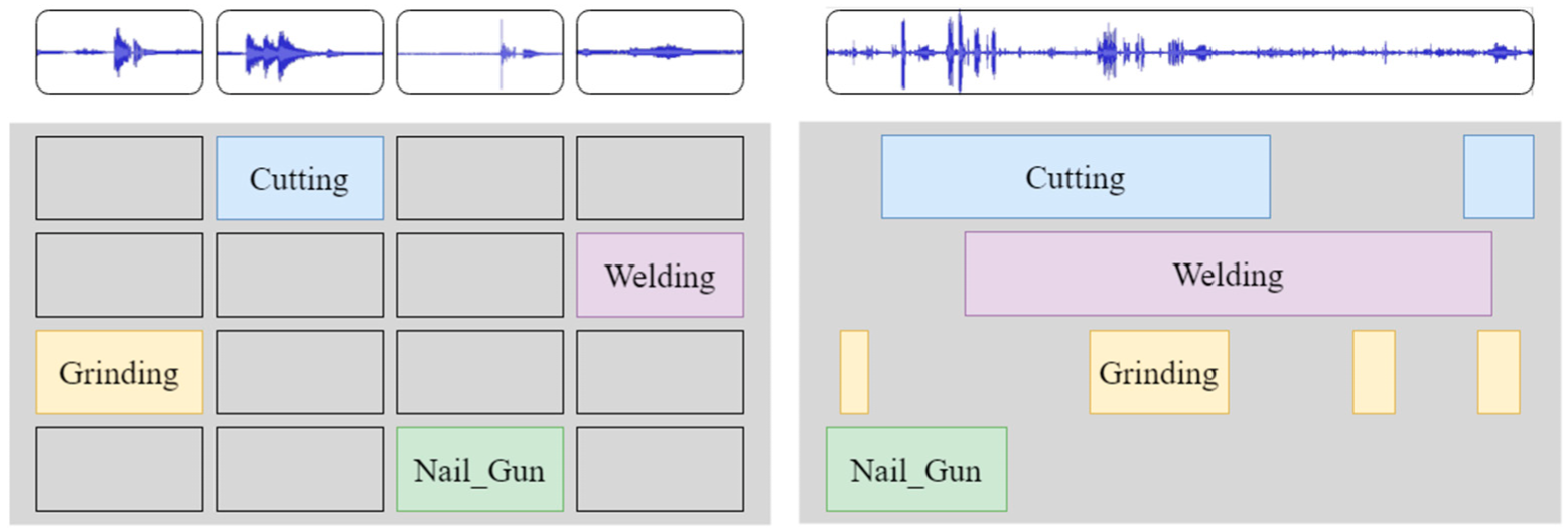
Prior studies of sound classifiers have mainly addressed issues associated with multi-class, namely, only one output class for each input [26]. These classifiers were used to identify different construction activities with the single-construction-sound input. Other applications include determining the type of the monitored equipment or determining whether the monitored target is in operation or idle. It indicates that the existing methods trained on data with only one activity sound at a time cannot be employed in a polyphonic construction environment [47]. Multi-label sound classifiers concurrently output multiple alternative categories for each input. The difference between multi-class and multi-label classification is shown in Figure 1. Although the multi-class classification model can only detect the most prominent sound occurrence within a monophonic sound sample, the proposed model aims to solve the multi-label classification issue for polyphonic overlapping sound samples.

The distribution feature of sound waves in the time domain, regarded as the temporal pattern, is governed by the individual sound source or the construction activity that produces the sound. For instance, the sound wave shape of spot and continuous weld is identical, but the former is produced discretely, while the latter happens continuously. Moreover, construction activities are significantly time-connected, therefore the extraction of temporal contextual information is crucial for the comprehension of construction scenarios. This suggests that to identify the specific construction activity, one has to recognize not only the category of construction sound but also its temporal pattern. The start and end times for such activities are also needed in the scheduling and other project management tasks. To this end, this method focuses on locating the start and finishing times for individual activities, as seen in Figure 2, which illustrates the comparison between our method and the existing research.

The presented research necessitates the development and training of models for sound event detection based on certain types of construction activities, without addressing the application of their models to other construction activities. Extending new classes is costly for traditional machine learning methods based on statistical learning since it often requires retraining the whole model. Due to the variety of construction sites, the model’s ability to generalize is essential for construction management. Different brands and models of construction equipment have varying acoustic qualities, and different construction sites often use various construction processes, etc., necessitating the adaptability of sound-based methods. In addition, the concept of transfer learning in deep learning has not yet been studied in the area, despite the fact that it is widely acknowledged as a successful method for improving the model’s adaptability to new tasks. To overcome this gap, the suggested model integrates CNN and RNN into an end-to-end model that eliminates redundant and step-by-step methods. This model is pre-trained using publicly accessible audio datasets, and its adaptability to extra tasks is evaluated. The suggested deep learning model is very adaptable for use in extra construction applications.

3. Methodology

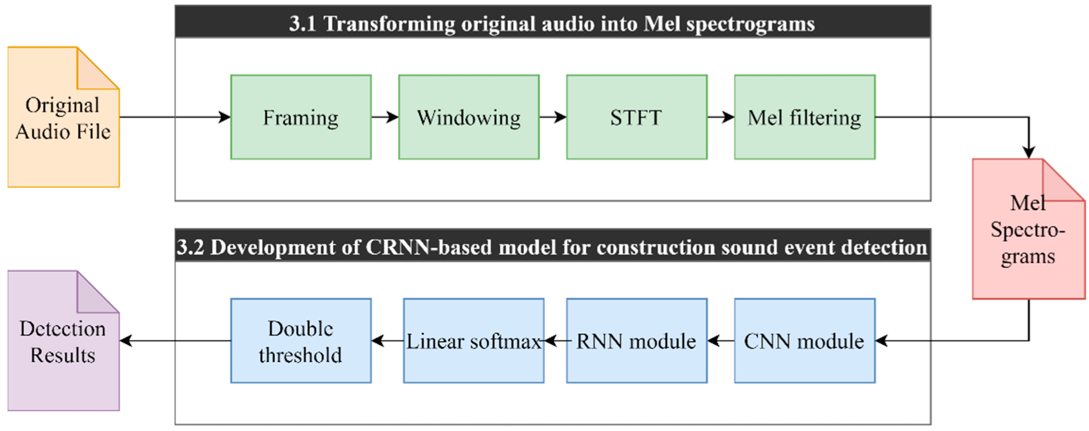
This section summarizes the construction of a sound-based deep learning model for construction activity detection. Firstly, the original audio signal was converted into the time-frequency spectrogram as the input of the model. After that, we developed a CRNN model that is composed of a five-layer CNN and a variant of RNN called GRU. Finally, the approach of pre-training and fine-tuning on the target task is revealed. The process of the proposed methodology is shown in Figure 3.

3.1. Transforming Original Audio into Mel Spectrograms

Audio feature extraction can be categorized as time-domain features, frequency-domain features, and time-frequency representation. The capacity of the deep learning method to extract DAFs from time-frequency representations offers a major benefit. The Mel spectrogram, as one of the time-frequency representations, is used as the input in this research. To extract the appropriate Mel spectrogram from the original audio file, a series of processing steps are carried out, including framing, windowing, short time Fourier transforms (STFTs), and Mel filtering. Details are shown in Figure 4.

The typical sound frames are between 10 and 30 ms, and an overlapping segmentation approach is utilized to eliminate discontinuities between frames. Segmentation is accomplished by multiplying the signal with a finite length windowing function. The function equation of Hamming window used in this research is shown below.

$$\omega \left(n\right)=\left\{\begin{array}{c}0.54-0.46\cos \frac{2\pi n}{N-1}, 0\le n\le N-1\\ 0, n < 0 or n > N-1\end{array}\right.$$

(1)

where N denotes the length of the window, and n denotes the audio signal of the current frame.

Due to the fact that the sound signal is a one-dimensional time-domain signal, it is intuitively difficult to express the pattern of frequency variation. Many time-frequency analysis techniques have been developed, including STFTs. The below is a functional representation of the STFTs, with n representing discrete time and $w\left(n-m\right)$ representing the window function.

$$X_n\left(e^{j\frac{2\pi k}{N}}\right)={{\displaystyle \sum }}_{-\infty }^{+\infty }x\left(m\right)w\left(n-m\right)e^{-j\frac{2\pi km}{N}}$$

(2)

The human ear can sense frequencies between 20 and 20,000 Hz, while the frequency perception does not increase linearly. There is an auditory masking effect, which means that the louder sound could alter the aural impression of the quieter sound [23]. Following the Mel filter, the auditory features most congruent with human ear perception will be retrieved [21]. The Mel filter bank is a triangular filter bank based on the Mel scale, and satisfies the following conversion equation.

$$Mel\left(f\right)=2595\times \lg \left(1+\frac{f}{700}\right)$$

(3)

$Mel\left(f\right)$ denotes Mel’s perceived frequency and $f$ denotes the real frequency. The frequency response of the Mel filter bank based on the Mel scale is defined as follows:

$$H_m\left(k\right)=\left\{\begin{array}{c}0, k<f\left(m-1\right)\\ \frac{k-f\left(m-1\right)}{f\left(m\right)-f\left(m-1\right)}, f\left(m-1\right)\le k\le f\left(m\right)\\ \frac{f\left(m+1\right)-k}{f\left(m+1\right)-f\left(m\right)}, f\left(m\right)\le k\le f\left(m+1\right)\\ 0, k>f\left(m+1\right)\end{array}\right.$$

(4)

3.2. Development of CRNN-Based Model for Construction Sound Event Detection

The model contains five parts: (1) the feature extractor extracts a time-frequency log-Mel spectrogram as the input to the convolutional layers; (2) the convolution layers transform the spectrogram into feature maps; (3) recurrent layers with a fully connected layer give the estimated event presence probabilities for each frame from the input feature maps; (4) during training, an additional aggregation layer transforms the estimated frame event probabilities into the whole clip event probability; (5) during inference, post-processing is utilized to obtain the predicted event activities. An illustration of the system structure is shown in Figure 5.

Feature extractor: in this work, we use a 64-dimensional log-Mel spectrogram as the input feature. STFT is performed with a window size of 40 ms, a window shift of 20 ms and an FFT size of 2048 [48].

Convolutional layers: the CNN part consists of five convolutional blocks. Each block contains a batch normalization layer, a 2D convolutional layer and an activation layer. Unlike common ReLU, LeakyReLU with a negative slope of −0.1 is used as the activation. The convolution layer uses 3 × 3 kernels with 1 × 1 zero-padding, so that the feature map size remains unchanged before and after the layer. The convolution channel numbers are 32, 128, 128, 128 and 128. As Figure 5 shows, there are three pooling layers between the convolution blocks. Non-overlapping L4 pooling is used:

$$L_p\left(x\right)=\sqrt[p]{{{\displaystyle \sum }}_{x\in K}{x}^p }$$

(5)

the elements within the kernel x∈K are aggregated by L4 pooling. The pooling kernels are two-dimension: 2 × 4, 2 × 4 and 1 × 4. After the convolution layers, the input spectrogram $X\in {ℝ}^{T\times F}$ is transformed into a feature map $\mathcal{H}\in {ℝ}^{128\times \frac{T}{4}\times \frac{F}{64}}$. Since F = 64, the frequency dimension is reduced to 1 and we reshape it into ${\mathcal{H}}^{\prime }\in {ℝ}^{\frac{T}{4}\times 128}$. An additional dropout layer with a dropout probability of 30% is appended to the convolution layers to prevent over-fitting.

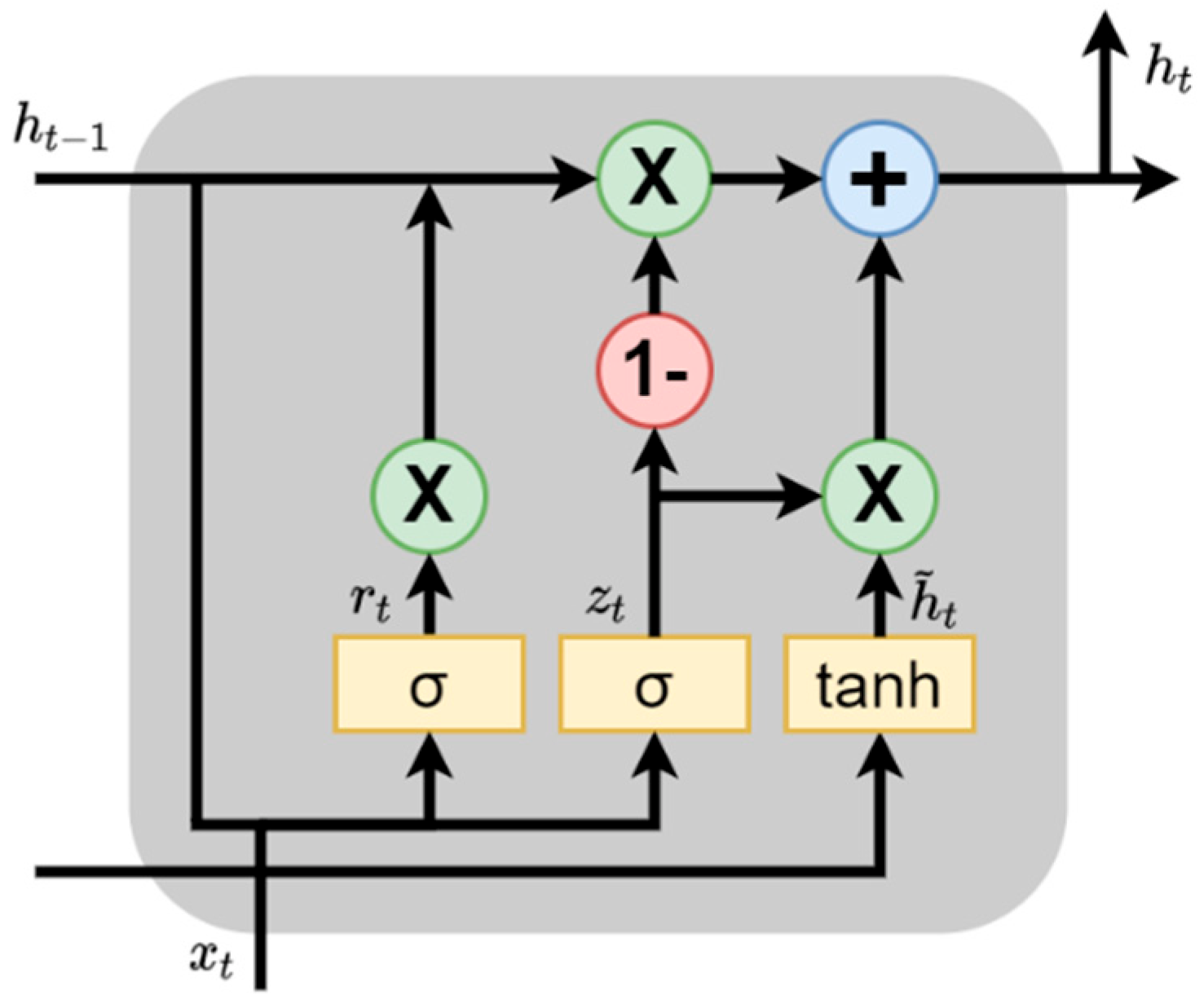
Recurrent layers: The feature maps ${\mathcal{H}}^{\prime }\in {ℝ}^{\frac{T}{4}\times 128}$ are fed to an RNN for further encoding. It is viewed as a sequence containing $\frac{T}{4}$ time steps with an embedding size of 128. A single-layer bidirectional gated recurrent unit (BiGRU) is used as the RNN. For both directions, BiGRU updates the hidden state of the current time-step $h_t$ based on the previous hidden state $h_{t-1}$ and the current input $x_t$, as shown in Figure 6:

$$z_t=\sigma \left(W_{xz}{x}_t+W_{hz}{h}_{t-1}\right)$$

(6)

$$r_t=\sigma \left(W_{xr}{x}_t+W_{hr}{h}_{t-1}\right)$$

(7)

$${\tilde{h}}_t=\tanh \left(W_{xh}{x}_t+r_t\odot \left(W_{hh}{h}_{t-1}\right)\right)$$

(8)

$$h_t=\left(1-z_t\right)\odot {\tilde{\mathbf{h}}}_t+z_t\odot h_{t-1}$$

(9)

The hidden dimension is 128, so the output $\mathcal{O}\in {ℝ}^{\frac{T}{4}\times 256}$. The RNN enhances the model’s ability to accurately detect audio events through the time axis. After RNN, a fully-connected layer is employed to transform the embeddings into event probability predictions:

$$y_t=\sigma \left(\mathrm{FC}\left({\mathcal{O}}_t\right)\right)$$

(10)

where $y_t\in {ℝ}^C$ i is the estimated event probabilities of C classes for frame t.

Aggregation layer: During training, only clip-level labels are available, so the frame-level outputs are aggregated to obtain clip-level outputs for back propagation. Formally, for event $e$, its clip-level probability $y\left(e\right)\in \left[0, 1\right]$ is aggregated by linear softmax:

$$y\left(e\right)=\frac{{{\displaystyle \sum }}_t^T{y}_t{\left(e\right)}^2}{{{\displaystyle \sum }}_t^T{y}_t\left(e\right) }$$

(11)

Linear softmax is a non-parameterized aggregation approach, which adopts the frame-level probability itself as the averaging weight. It is robust to both long and short sound events.

Post-processing: During inference, post-processing is required to transform the estimated frame-level probability $y_t\left(e\right)\in \left[0, 1\right]$ into a binary prediction ${\overline{y}}_t\left(e\right)\in \left\{0,1\right\}$. It can also smooth the outputs (e.g., removing fragmented outputs). Before the binarization, we first employ a parameter-free upsampling operation vis linear interpolation to restore the original temporal input resolution. The probability sequence with $\frac{T}{4}$ frames are interpolated to T frames. The double threshold is used as the post-processing method [13]. It is defined by two thresholds; that is, ${\varphi }_{high}$ and ${\varphi }_{low}$. First, the output probability sequence is swept through an output probability sequence, and all values larger than ${\varphi }_{high}$ are marked as valid predictions. Then, the predictions are expanded to its adjacent regions, whose values are larger than ${\varphi }_{low}$.

3.3. Pre-Training and Transfer Learning

To the best of our knowledge, previous research on detecting construction activities have not taken the pre-training process into account. The existing publicly accessible sound datasets are mostly for domestic and street settings, but do not cover construction environments. Considering the potential improvement of model training via transfer learning or self-supervised learning [49], this study investigated the impact of pre-training the model using the public sound database. In transfer learning, the source and target tasks may have totally distinct data fields and task settings, but the knowledge required to perform these tasks is the same [50]. An obvious assumption is that the source and target tasks share a prior distribution of model parameters or hyperparameters.

According to this inspiration, transfer learning is utilized to pre-train the model. The publication of AudioSet, a dataset encompassing 527 sound categories and more than 5000 h of recordings, is a watershed moment for audio pattern recognition [51]. In order to optimize the performance, the proposed model is pre-trained based on AudioSet. It is the most large-scale weakly-annotated sound event dataset. There are 2.04 M audio clips (about 1.9 M available) for training. Each audio clip has a duration of at most 10 s and is annotated by at least one sound event. We pre-train the CRNN on it using a balanced data sampling strategy and binary cross entropy loss. The pre-training setups are the same as PANNs [52]. The model is pre-trained using one NVIDIA GTX1080Ti graphics card for three days. After pre-training, the model achieves a mAP (mean Average Precision) of 0.226, an AUC (Area Under Curve) of 0.929, and a d-prime of 2.080 on the AudioSet evaluation set.

4. Data Preparation and Training

4.1. Data Collection

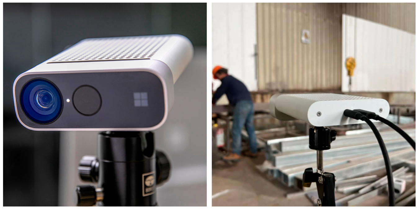
There are already a small number of sound datasets, such as TUT-SED 2016, TUT-SED 2017, DCASE 2017, and DCASE 2018. The available dataset provides only acoustically labeled events for street and residential settings, necessitating the collection of sound data pertaining to construction activities for model training and validation. Along with audio, the video should be captured concurrently to facilitate manual annotation. The Azure Kinect not only has a depth sensor and camera for computer vision applications, but it also has a seven-microphone array for far-field voice and sound capture. Figure 7 shows the equipment.

Our data set was collected in Hele Technology’s plant in Suzhou, China, a steel modular construction factory. The construction operations on this site are quite similar to those on a steel construction site, mainly including the construction of primary steel structures, the construction of secondary structures, and the assembly of various construction systems. The construction products usually manufactured by this factory are modular buildings with steel mainframes. The main work of manufacturing the primary frames is the machining and welding of the steel framework. The partition walls are made of oriented strand board (OSB), and they are attached to the mainframe with nail guns. The external finish consists of panels nailed to the inside OSB. The research examined five construction activities, namely welding, cutting, hammering, nailing, and grinding, all of which frequently occur in this factory. The five types of sound shown in Figure 8 were chosen because they are directly tied to the construction process and have distinct acoustic features. Plant management, construction staff, and our field observations corroborated these rationales.

Between November 2021 and January 2022, the plant finished the manufacturing process for two batches of modular buildings. Throughout the production process, we captured audio and video. The sound included in the dataset were created naturally throughout the building process by construction workers who were not coached by us. To enhance production efficiency, several building modules were manufactured concurrently in the factory using asynchronous construction, which often results in many separate construction operations happening concurrently.

4.2. Data Collection

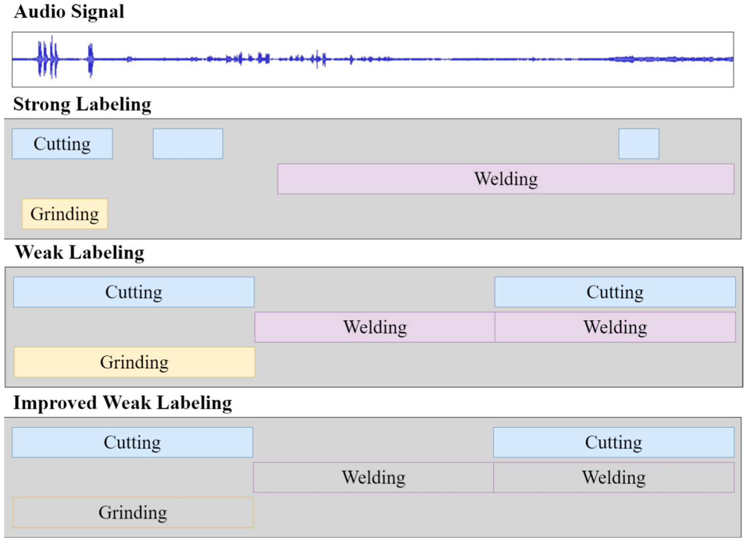
In order to effectively mark the sound events, it is required to not only identify each unique occurrence of the event category, but also to provide a detailed description of their start and end times. Weak labeling only involves the calibration of the kind of sound events that occur within a specific time period, rather than complete start and end times, which saves a substantial amount of time during the annotation process [53]. The difference between strong and weak labeling can be found in Figure 9. Considering the huge differences in the number of various sounds encountered on the construction sites, we developed a unique strategy to supplement the training samples with under-represented construction activities. The large variability in the number of different activities in the data set species was also reflected in the study reported by Rashid et al. and this variability may introduce bias into model training [13]. The specific training set we defined taught the model simply whether a certain sort of sound (e.g., cutting) occurs at a given time, regardless of other forms of sound. This training procedure was eventually accomplished by restricting backpropagation. Only the loss of the certain sound category was backpropagated for training the model, while losses of other classes are ignored.

The training set divides the collected audio data into 10 s segments, generating a total of 1136 test segments, the number of which is shown in

Table 1. The number of 10 s audio segments covering individual construction activities.

	Cutting	Grinding	Hammering	Nail_Gun	Welding
Number of Instances	306	746	343	237	284

for each job type. Moreover, we labeled one test set as the basic fact for evaluating the performance of the model, which is in line with the principles of strong annotation. These annotation methods are facilitated by video footage shot concurrently with the audio data.

A varying number of activities are labeled on the same 10 s sound segment for the training set. In another instance, no activity of interest is labeled on the sound segment, implying that there is no activity of interest during those periods. These segments are necessary for the model to respond to ambient background noise, and may even be thought of as punitive inputs to the background noises (both white noise and uninteresting secondary construction activities).

4.3. Training

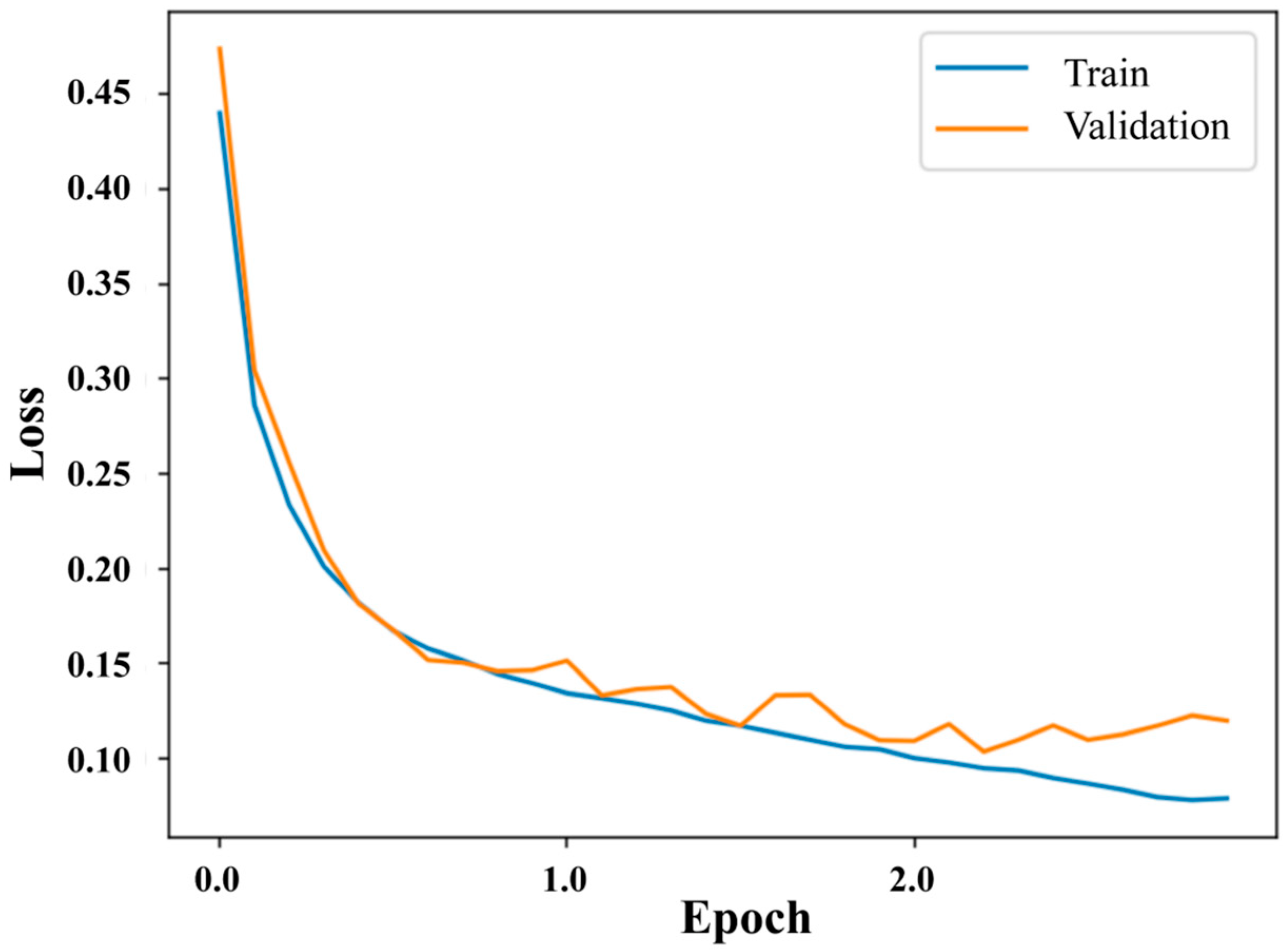
To train the proposed model on the annotated dataset, the training set was divided into a training subset and a validation subset in a 9:1 ratio. Since the dataset is unbalanced and multi-labeled, this study applied an iterative stratification method [54] to provide a balanced distribution of labels in both the training and validation subsets. SpecAugment [55] by time masking and frequency masking is used for data augmentation. We use a batch size of 64, and an Adam [56] optimizer with an initial learning rate of 0.001 for training. If the loss on the validation set does not improve for 3 epochs, the learning rate is multiplied by 0.1. The model is trained on a single NVIDIA GTX1070Ti card for at most 100 epochs with an early stop of 7 epochs (Figure 10 shows the loss curve of training work).

5. Results

This section defines four metrics, i.e., Tagging F1-Score, Segment F1-Score, Event F1-Score, and mAP to evaluate the modeling performance. The effect of the two threshold values, ${\varphi }_{high}$ and ${\varphi }_{low}$, on the model’s performance is also assessed. Following that, the model’s overall performance is analyzed and discussed. Finally, the performance of the proposed model to that of existing models is compared.

5.1. Metrics

Originally developed for the application in the field of information retrieval to evaluate search, document classification, and query classification performance, the F1-Score has evolved into a critical indicator for assessing machine learning systems. The F1-Score is also a commonly employed indicator of polyphonic evaluation in sound event detection. Precision ($P$) and Recall ($R$) are the primary metrics for assessing information retrieval, which constitutes the basis of the F1-score calculation. $P$ and $R$ are also called positive prediction value and sensitivity in classification issues, and they are defined as follows [25].

$$P=\frac{\mathrm{TP}}{\mathrm{TP}+\mathrm{FP}}$$

(12)

$$R=\frac{\mathrm{TP}}{\mathrm{TP}+\mathrm{FN}}$$

(13)

$$\mathrm{F}1=\frac{2P\times R}{P+R}$$

(14)

where:

TP means the number of true positives classified by the model; FP means the number of false positives classified by the model; and FN means the number of negatives classified by the model.

To assess the multi-class classification tasks, the basic F1-score, called tagging F1, can be employed. This metric is used to assess the model’s ability to properly recognize the existence of an event inside an audio clip, which is commonly applied in previous research. However, it cannot be used to validate the model’s temporal localization of the target activity.

According to the statistical unit, the F1-score can be further divided into a Segment F1-score or an Event F1-score. The Segment F1-score is calculated based on segment-level precision and recall [57]. The Event F1-score specifies a model’s capacity to estimate the duration of an event (i.e., predicting the start and end) [58]. Segment F1- score and Event F1- score are stricter than Tagging F1-score. Another metric, mAP, is used to evaluate the performance of our model in multi-label classification. Its value depends on the area covered by the Precision-Recall Curve.

5.2. Thresholds Analysis

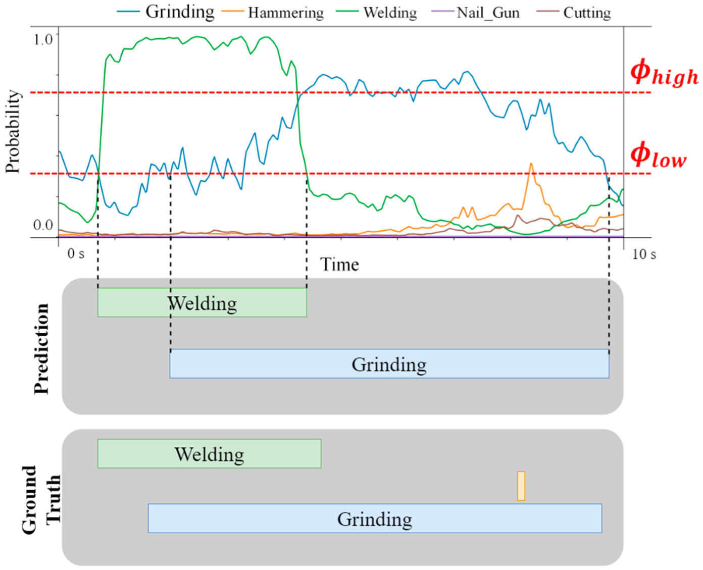
Thresholds ${\varphi }_{high}$ and ${\varphi }_{low}$, are crucial to the post-processing of the model. After Linear softmax, the independent clip-level probability ${\overline{y}}_t\left(e\right)\in \left\{0,1\right\}$ is acquired for each construction activity, as illustrated in Figure 11.

The horizontal axis in Figure 12 indicates the timing, the vertical axis represents the clip-level F1-scores, and the colored curves represent ${\overline{y}}_t\left(e\right)$ corresponding to distinct construction activities at a specific point. Using two thresholds to filter the output is more stable than a single threshold. ${\varphi }_{high }$ is used to set the minimum probability value for output, whereas ${\varphi }_{low}$ is used to obtain the event’s beginning and end boundaries. All predictions with values greater than ${\varphi }_{high }$ are considered valid. The searching is then shifted to neighboring locations in order to find those with values greater than ${\varphi }_{low}$.

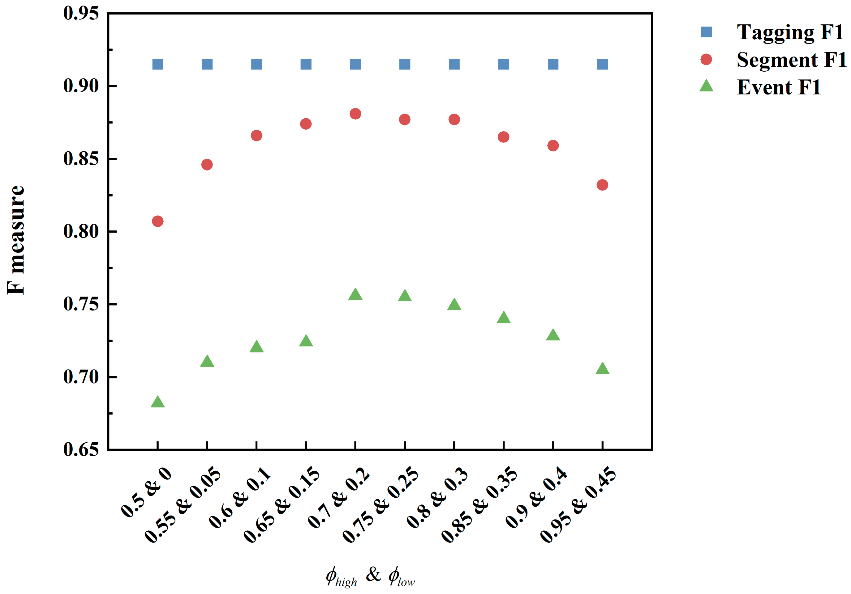
Changes in both ${\varphi }_{high }$ and ${\varphi }_{low}$ will have an effect on the model’s ultimate performance. On the basis of these principles, various combinations of ${\varphi }_{high }$ and ${\varphi }_{low}$ were tested, as shown in Figure 12. The model performs optimally when ${\varphi }_{high }$ and ${\varphi }_{low}$ are set to 0.7 and 0.2, respectively, among the 10 candidate combinations.

5.3. Performance Evaluation

In this section, the performance of the model was evaluated through four kinds of metrics, namely, Tagging F1, Segment F1, Event F1 and mAP. The test set data was collected in the same steel modular construction factory as the training set. The full test set was collected over a period of 2 h 32 min at seven separate time points. In addition, these audio files have been strongly labeled by means of video assistance, which gave the classification, start and end times of each independent event.

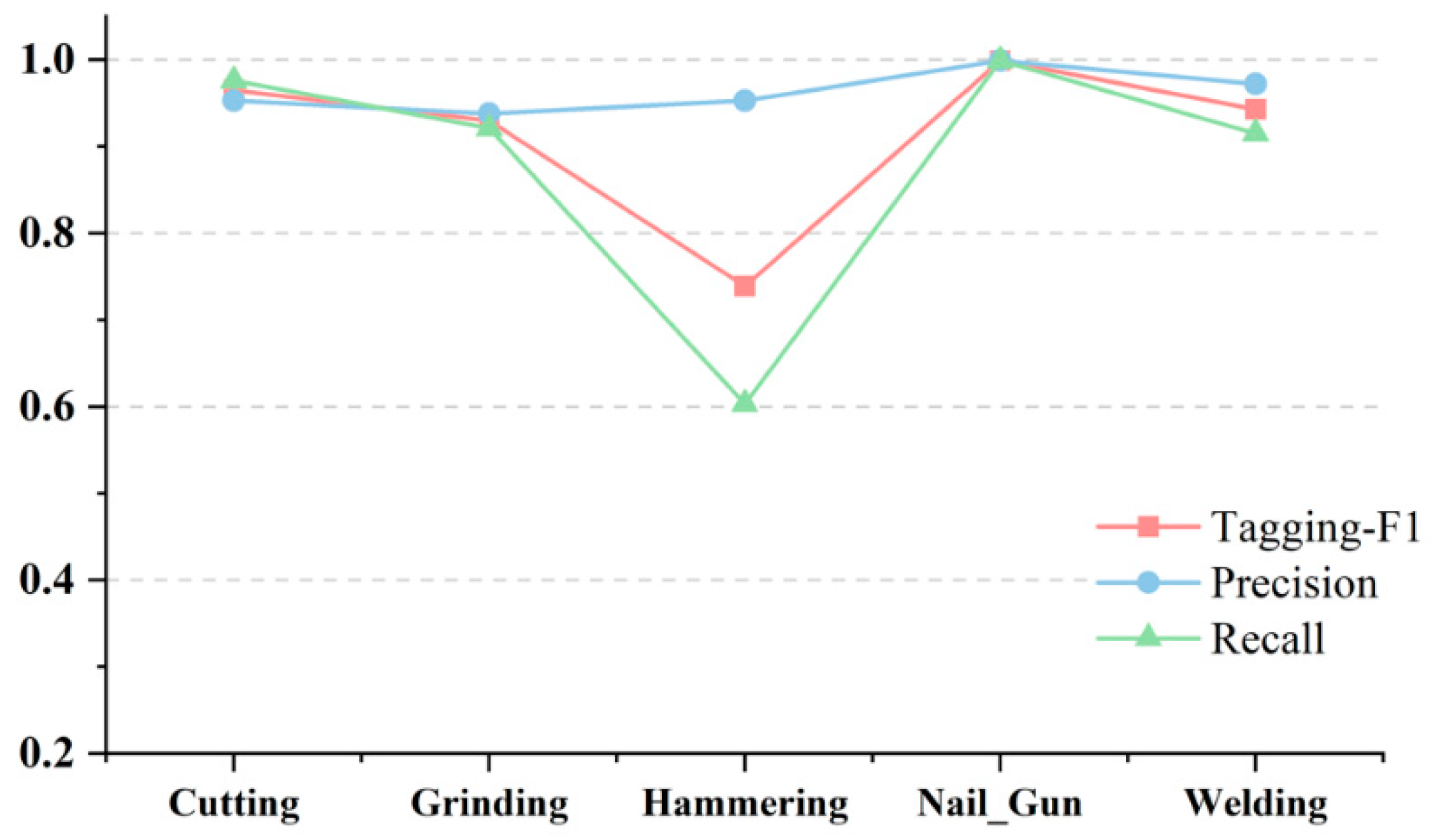
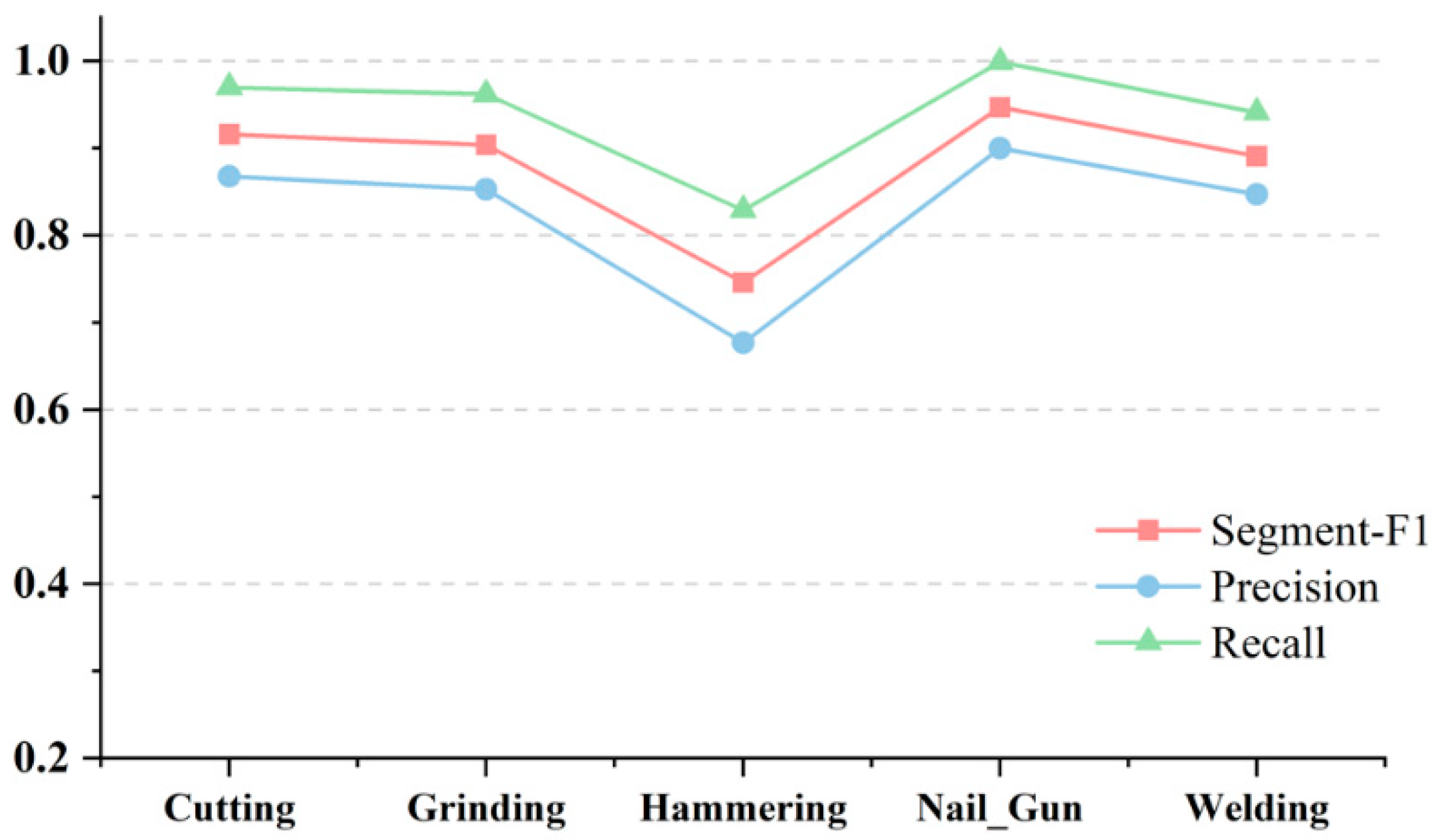
Figure 13 illustrates the whole test procedure. A video demonstrating the output of the model is supplied as Supplementary Materials. Overall, we obtained a Tagging F1-score of 91.5% (precision of 96.3%, recall of 88.3%), a Segment F1-score of 88.1%, an Event-F1 score of 75.6%, and the mAP was 0.972, respectively. The details are shown in

Table 2. The F1-score, precision and recall values.

	F-Measure	Precision	Recall
Tagging based	91.5%	96.3%	88.3%
Segment based	88.1%	82.9%	94.0%
Event based	75.6%	75.8%	75.5%

, and Figure 14, Figure 15 and Figure 16.

As can be seen from Figure 14, Nail_ Gun achieved the highest Tagging F1-score of 99.9%, which was followed by Cutting, Welding, and Grinding, with scores of 96.5%, 94.3%, and 93.0%, respectively. Hammering’s Tagging F1-score was only 73.9%, which was the lowest among all construction activities. In the event of Hammering, false positives accounted for a large proportion, which might be attributed to the fact that there were many noise activities similar to Hammering at the construction site, such as the sound of metal components falling. In addition, noise mingling caused false detections.

In the evaluation of the Segment F1-score, Nail_Gun had the highest score of 94.7%. However, Hammering still had the lowest score of 74.6%. The score of Welding in this item (89.1%) ranked behind Grinding. One of the main reasons was that the precision of Welding dropped to 84.7%, which might be due to the low volume of sound related to welding events. It tended to lead to wrong judgments in scenes with severe overlapping sounds.

The results of Welding and Hammering in the Event F1-score further decreased to 65.4% and 43.0%. Compared with Cutting and other continuous activities, the sounds of Welding and Hammering tend to be intermittent and random, making it difficult to locate the time accurately. Moreover, the sound of Hammering was short, and the predicted offset was more likely to lead to a decline in accuracy.

It can be found from the above analysis that there were obvious differences in the recognition accuracy and temporal locating accuracy of different construction sound types. An obvious difficulty was that some construction sounds were extremely similar, which influenced the identification of some construction activities, For example, the sound of metal knocking and metal components falling were prone to be mixed-up. In addition, due to sound volume differences, the anti-interference ability of different sounds in the complex sound environment was also different.

5.4. Benchmark

Although no publicly released construction dataset was available for comparison, the performance of this model compared to existing ones, in terms of their applicability and versatility, was tested first. The training dataset consists of an unselected construction sound captured in a real mixed-sound environment, while previous research has utilized training data collected or selectively picked in a single-sound environment. In addition, the methodology in this study is designed for multi-label classification, with each classification producing an independent output. In order to carry out the like-for-like comparison, we altered the post-processing settings and the test set to fit previous research cases. For post-processing, the sound event with the maximum estimated probability as the prediction result was picked. We chose segments from the given test set that included just one construction activity of interest. Following that, we assessed if the proposed model could perform multi-class classification tasks as the counterpart cases do. With the exception of hammering (90%), all activities had a classification precision of more than 97% and indicated robust recalls (see

Table 3. The F1-score, precision and recall for individual construction activities.

Activities	F1	Precision	Recall
Cutting	99%	97%	99.9%
Grinding	98%	99.9%	96%
Hammering	93%	90%	96%
Nail_Gun	99.99%	99.99%	99.99%
Welding	99%	98%	99%

). As indicated in

Table 4. The performance of our method compared with prior studies in multi-class classification tasks.

Ref.	Task	Accuracy
[32]	Equipment classification	>90%
[12]	Equipment classification	17~98%
[33]	Equipment classification	Up to 99%
[34]	Equipment classification	Up to 88%
[16]	Construction activities classification	Up to 94.3%
[20]	Construction activities and equipment classification	Up to 93.16%
[39]	Equipment classification	97%
[22]	Equipment classification	97.79% for F1-score
[13]	Modular construction activities classification	97% for F1-score
[22]	Equipment classification	Up to 98%
[21]	Equipment classification	Up to 99.45%
Ours	Construction activities classification	Up to 99.9%

, we attained an overall performance that outperforms prior research.

6. Discussion

In this chapter, the investigation related to model interpretability and versatility will be presented. The innovation features and their contribution on the model performance is considered in the ablation study, including the influence of pre-training, CNN module, RNN module and the impact of double threshold. In the extended experiment, the employability of applying the proposed model to other construction environments and construction activities is further investigated.

6.1. Ablation Study

An ablation study typically refers to removing some features of the model or algorithm and observing their impact on performance. Through ablation study, how different modules in the model serve their functions will be identified, which provides information on a certain degree of interpretability for the deep learning model. The ablation study is carried out with reference to four parts, namely, pre-training, CNN, RNN, and double threshold. It can be found from

Table 5. The F1-score and mAP for ablation study.

	Tagging F1	Segment F1	Event F1	mAP
CRNN	91.5%	88.1%	75.6%	0.972
Case 1: Without Pre-training	58.7%	80.6%	33.5%	0.762
Case 2: Without CNN	64.4%	64.6%	36.1%	0.674
Case 3: Without RNN	69.2%	68.7%	5.8%	0.898
Case 4: Median Filtering	91.5%	87.2%	60.7%	0.972

that the examined four modules (pre-training, CNN, RNN, and double threshold) have an important impact on the performance of the model.

The most significant impact on activity classification accuracy is the Case 1 without pre-training, the model’s Tagging F1 drops from 91.5% to 58.7%. Through transfer learning, the pre-trained models are considered to accelerate the training of the model parameters. Although the pre-training data chosen is not associated with the construction process, the proposed model still benefits from the basic features learned from the pre-training data.

In other cases regarding the acoustic classification of construction activities, the CNN or RNN module is employed alone. In the proposed model, the CNN and RNN modules are combined, to be applied to the detection of construction activities. The impact of two modules, i.e., CNN and RNN, on the performance of the model, and the benefits of using the combined model, are studied through the ablation study as well. After removing the CNN (Case 2) or RNN module (Case 3), the Tagging F1 of the model is only 64.4% and 69.2%. In particular, after removing the RNN module, the Event F1-score of the model is only 5.8%, which means that the RNN module plays a critical role in locating the start and end times of activities. The mAP values reduce to 0.674 and 0.898, respectively, when the CNN or RNN module is removed. Although the removal of the RNN module has a substantial influence on Event F1, the mAP does not fall considerably. This suggests that the RNN module is crucial for identifying the start and end of events but contributes little to determine the classification accuracy of events. Meanwhile, the CNN module has a considerable influence on mAP performance, implying that the CNN module is critical for accurate event classification.

After changing the double threshold to medium filtering with single threshold, the Tagging F1-score of the model is not affected, but the Event F1-score decreases to 60.7%. Such results indicate that the double threshold is also of great significance in judging the start and end times of the construction activities.

6.2. Extended Experiment 1: Applying in New Construction Environment

Deep learning methods are typically trained and tested in batches on models using the same dataset. Image classification studies have shown that models trained and tested on the same open image datasets (CIFAR-10, ImageNet) will perform up to 15% better than those tested on a new dataset [42]. In this part, we conducted an extended experiment to evaluate the adaptability of the proposed model to different construction environments. The data used for the test are from public videos and audio on YouTube.

The detection accuracy of learned instances in a new construction environment is considered. The audio and video selected are from a decoration site, where hammering and cutting activities occurred frequently. In addition, there are other construction activities that have not been learned, such as hand sawing wood. The model trained in the presented study has a construction activity detection application in this case.

In this decoration construction setting, there are only two types of model-trained construction activities, namely, Cutting and Hammering (see

Table 6. The F1-score, precision and recall for extended experiment 1.

	Tagging F1	Precision	Recall
Cutting	77.4%	80.0%	75.0%
Hammering	83.5%	76.8%	91.4%

). Results illustrate that the detection performance of cutting events decrease to a certain extent. The Tagging F1-score is 77.4%, while the accuracy is 80.0%. The reason for the drop may be that there are some other activities, such as drilling, in this new construction environment, that may interfere with the identification of cutting events. These types of construction activities, which our model has not been trained in, may affect the accuracy of the identification of some construction tasks. Another interesting observation is that even the detection results of hammering are improved, and the Tagging F1-scores rise to 83.5%, thanks to the high recall rate (91.4%). The high-frequency hammering activities are included in this decoration environment, and the noise created by falling metal objects is significantly less than that of the modular construction environment, which may also be the reason for the improvement in the results.

The above results indicate that the performance of our model still remains consistent, even when it is applied to a new construction environment that may include different types of background noise. Different environments may have varying influences on the performance of construction tasks, and these effects are not necessarily all negative.

6.3. Extended Experiment 2: Applying a New Construction Activity

In the second study, the learning ability of the proposed model for new construction tasks is considered. The audio selected here still comes from the same decoration scene. We employed sound data collected at different times in the same construction setting as the training set and used the suggested improved weak labeling approach to identify segments of Hand_Sawing_Wood events occurring within three hours. Hand_Sawing_Wood events were tagged 296 times in the training set. We employed the model for testing in a test set consistent with Experiment 1 after it was retrained. The Tagging F1-score of Hand_Sawing_Wood was 99.99% (

Table 7. The F1-score, precision and recall for extended experiment 2.

	Tagging F1	Precision	Recall
Hand_Sawing_Wood	99.9%	99.9%	99.9%

).

This work suggests that the method in this study can be equally applied to other activity detection tasks after labeling a small number of samples. The suggested improved labeling approach is applicable throughout the procedure without annotating activities we have already trained, which will also significantly mitigate the difficulty for engineers to utilize this method. This has implied that our technology can be applied to various types of construction activity monitoring at a low cost.

7. Conclusions

This research has developed a deep learning-based model for identifying and monitoring construction activities by detecting their sounds. We integrated CNN and RNN to establish an improved model, which can capture robust acoustic features from the time-frequency spectrogram. This model can be used to complete the event classification and temporal localization tasks for sound inputs. The novel features of this model include that it can detect and differentiate each single sound event from mingled acoustic sources containing background noises, as recorded in real construction scenarios.

In the validation cases, we collected a series of real construction sounds from a steel modular construction factory to train and test the proposed model. Four metrics were selected to evaluate its performance and results reveal an average Tagging F1-score of 91.5%, a Segment F1-score of 88.1%, an Event F1-score of 75.6% and a mAP of 0.972 for five different kinds of construction activities. This has indicated that the proposed model has outperformed the most published research. The ablation study highlights the respective contributions from each novel design feature, e.g., combining CNN and RNN, the introduction of a pre-training process, and the selection of dual thresholds as the output in post-processing. Two extended experiments confirm the versatility of the proposed approach and the applicability to a wider range of construction activities and settings.

In view of the above observations, we can see that the developed model offers a viable solution to detect varieties of construction activities in a real-time, complete, accurate and swift manner. It is designed for practical engineering and, thus, the novel features, such as less demand for training sets and the ease of data labelling, can effectively reduce the learning and application costs.

An acoustics modality technique has evident benefits in construction monitoring as evidenced by the absence of capturing blind spots, affordable equipment costs and low computing resource needs; and yet, the inherent limitation of such a technique should also be noted. For instance, some construction activities lack distinctive or distinguishable construction sounds. Furthermore, sound alone cannot capture the same level of detail as vision-based or other detection methods for some activities. As a result, we will investigate integrating machine audition with other methods in order to perform comprehensive and precise monitoring tasks for construction by leveraging the respective strengths of different modalities and mitigating the negative effects caused by disturbing environmental factors.

Moreover, we intend to employ the suggested methodology to develop a digital twin for construction monitoring. Future research will focus on sound event localization and detection techniques in order to match identified construction activities with their spatial positions inside the BIM model. This involves combining two types of tasks into one, i.e., concurrently mining the distribution patterns of sound events of interest in time and location in order to conduct a more comprehensive acoustic scene analysis. The sound-based approach is expected to assist digital twins in facilitating enhanced productivity monitoring, anomalous sound detection, and safety management, among other capabilities.

References

1. Golparvar-Fard, M.; Peña-Mora, F.; Savarese, S. Monitoring changes of 3D building elements from unordered photo collections. In Proceedings of the IEEE International Conference on Computer Vision, Barcelona, Spain, 6–13 November 2011; pp. 249–256. [Google Scholar]
2. Navon, R.; Sacks, R. Assessing research issues in Automated Project Performance Control (APPC). Autom. Constr. 2007, 16, 474–484. [Google Scholar] [CrossRef]
3. Rao, A.S.; Radanovic, M.; Liu, Y.; Hu, S.; Fang, Y.; Khoshelham, K.; Palaniswami, M.; Ngo, T. Real-time monitoring of construction sites: Sensors, methods, and applications. Autom. Constr. 2022, 136, 104099. [Google Scholar] [CrossRef]
4. Ekanayake, B.; Wong, J.K.-W.; Fini, A.A.F.; Smith, P. Computer vision-based interior construction progress monitoring: A literature review and future research directions. Autom. Constr. 2021, 127, 103705. [Google Scholar] [CrossRef]
5. Paneru, S.; Jeelani, I. Computer vision applications in construction: Current state, opportunities & challenges. Autom. Constr. 2021, 132, 103940. [Google Scholar]
6. Reja, V.K.; Varghese, K.; Ha, Q.P. Computer vision-based construction progress monitoring. Autom. Constr. 2022, 138, 104245. [Google Scholar] [CrossRef]
7. Ryu, J.; Seo, J.; Liu, M.; Lee, S.; Haas, C.T. Action Recognition Using a Wristband-Type Activity Tracker: Case Study of Masonry Work. In Construction Research Congress; ASCE: Reston, VA, USA, 2016; pp. 790–799. [Google Scholar]
8. Rashid, K.M.; Louis, J. Automated Activity Identification for Construction Equipment Using Motion Data from Articulated Members. Front. Built Environ. 2020, 5, 144. [Google Scholar] [CrossRef]
9. Scislo, L.; Guinchard, M. Source Based Measurements and Monitoring of Ground Motion Conditions during Civil Engineering Works for High Luminosity Upgrade of the LHC; Canadian Acoustical Association: Montreal, QC, Canada, 2019. [Google Scholar]
10. Moselhi, O.; Bardareh, H.; Zhu, Z. Automated data acquisition in construction with remote sensing technologies. Appl. Sci. 2020, 10, 2846. [Google Scholar] [CrossRef] [Green Version]
11. Alaloul, W.S.; Qureshi, A.H.; Musarat, M.A.; Saad, S. Evolution of Close-Range Detection and Data Acquisition Technologies Towards Automation in Construction Progress Monitoring. J. Build. Eng. 2021, 43, 102877. [Google Scholar] [CrossRef]
12. Cheng, C.-F.; Rashidi, A.; Davenport, M.A.; Anderson, D.V. Activity analysis of construction equipment using audio signals and support vector machines. Autom. Constr. 2017, 81, 240–253. [Google Scholar] [CrossRef]
13. Rashid, K.M.; Louis, J. Activity identification in modular construction using audio signals and machine learning. Autom. Constr. 2020, 119, 103361. [Google Scholar] [CrossRef]
14. Sherafat, B.; Ahn, C.R.; Akhavian, R.; Behzadan, A.H.; Golparvar-Fard, M.; Kim, H.; Lee, Y.C.; Rashidi, A.; Azar, E.R. Automated Methods for Activity Recognition of Construction Workers and Equipment: State-of-the-Art Review. J. Constr. Eng. Manag. 2020, 146, 03120002. [Google Scholar] [CrossRef]
15. Cheng, M.A.; Anderson, D.V. A productivity forecasting system for construction cyclic operations using audio signals and a Bayesian approach. In Proceedings of the Construction Research Congress, New Orleans, LA, USA, 2–4 April 2018. [Google Scholar]
16. Zhang, T.; Lee, Y.-C.; Scarpiniti, M.; Uncini, A. A supervised machine learning-based sound identification for construction activity monitoring and performance evaluation. In Proceedings of the Construction Research Congress 2018, New Orleans, LA, USA, 2–4 April 2018; pp. 358–366. [Google Scholar]
17. Yong-Cheol, L.; Moeid, S.; Abbas, R.; Hyun Woo, L. Evidence-driven sound detection for prenotification and identification of construction safety hazards and accidents. Autom. Constr. 2020, 113, 103127. [Google Scholar] [CrossRef]
18. Deria, A.; Dominguez, P.J.C.; Choi, J.-W. An Audio-based Digital Twin Framework for Transportation Construction. In Proceedings of the Conference CIB W78, Luxembourg, 13–15 October 2021; pp. 11–15. [Google Scholar]
19. Dubnov, S. Computer audition: An introduction and research survey. In Proceedings of the 14th ACM International Conference on Multimedia, Santa Barbara, CA, USA, 23–27 October 2006; p. 9. [Google Scholar]
20. Lee, Y.-C.; Scarpiniti, M.; Uncini, A. Advanced sound classifiers and performance analyses for accurate audio-based construction project monitoring. J. Comput. Civ. Eng. 2020, 34, 04020030. [Google Scholar] [CrossRef]
21. Akbal, E.; Tuncer, T. A learning model for automated construction site monitoring using ambient sounds. Autom. Constr. 2022, 134, 104094. [Google Scholar] [CrossRef]
22. Scarpiniti, M.; Colasante, F.; Di Tanna, S.; Ciancia, M.; Lee, Y.-C.; Uncini, A. Deep Belief Network based audio classification for construction sites monitoring. Expert Syst. Appl. 2021, 177, 114839. [Google Scholar] [CrossRef]
23. Sherafat, B.; Rashidi, A.; Asgari, S. Sound-based multiple-equipment activity recognition using convolutional neural networks. Autom. Constr. 2022, 135, 104104. [Google Scholar] [CrossRef]
24. Kim, K.; Cho, Y.K. Effective inertial sensor quantity and locations on a body for deep learning-based worker’s motion recognition. Autom. Constr. 2020, 113, 103126. [Google Scholar] [CrossRef]
25. Mesaros, A.; Heittola, T.; Virtanen, T. Metrics for polyphonic sound event detection. Appl. Sci. 2016, 6, 162. [Google Scholar] [CrossRef] [Green Version]
26. Grandini, M.; Bagli, E.; Visani, G. Metrics for multi-class classification: An overview. arXiv 2020, arXiv:2008.05756. [Google Scholar]
27. DCase Community. DCASE 2022 Challenge. Available online: https://dcase.community/challenge2022/index (accessed on 6 September 2022).
28. Heittola, T.; Akr, E.; Virtanen, T. The Machine Learning Approach for Analysis of Sound Scenes and Events. In Computational Analysis of Sound Scenes and Events; Springer: Cham, Switzerland, 2018. [Google Scholar]
29. Wang, Y. Polyphonic Sound Event Detection with Weak Labeling. Ph.D. Thesis, Carnegie Mellon University, Pittsburgh, PA, USA, 2018. [Google Scholar]
30. Thomas, H.R.; Li, W.-H. Construction equipment identification via acoustical measurements. Autom. Constr. 1996, 5, 123–131. [Google Scholar] [CrossRef]
31. Cho, C.; Lee, Y.-C.; Zhang, T. Sound recognition techniques for multi-layered construction activities and events. In Computing in Civil Engineering; ASCE: Reston, VA, USA, 2017; pp. 326–334. [Google Scholar]
32. Cheng, C.F.; Rashidi, A.; Davenport, M.A.; Anderson, D. Audio Signal Processing for Activity Recognition of Construction Heavy Equipment. In Proceedings of the International Symposium on Automation & Robotics in Construction, Auburn, AL, USA, 18–21 July 2016. [Google Scholar]
33. Cao, J.; Huang, W.; Zhao, T.; Wang, J.; Wang, R. An enhance excavation equipments classification algorithm based on acoustic spectrum dynamic feature. Multidimens. Syst. Signal Process. 2017, 28, 921–943. [Google Scholar] [CrossRef]
34. Cao, J.; Wang, W.; Wang, J.; Wang, R. Excavation equipment recognition based on novel acoustic statistical features. IEEE Trans. Cybern. 2016, 47, 4392–4404. [Google Scholar] [CrossRef] [PubMed]
35. Sabillon, C.; Rashidi, A.; Samanta, B.; Davenport, M.A.; Anderson, D.V. Audio-based bayesian model for productivity estimation of cyclic construction activities. J. Comput. Civ. Eng. 2020, 34, 04019048. [Google Scholar] [CrossRef]
36. Mesaros, A.; Heittola, T.; Virtanen, T.; Plumbley, M.D. Sound event detection: A tutorial. IEEE Signal Process. Mag. 2021, 38, 67–83. [Google Scholar] [CrossRef]
37. Cakir, E.; Ozan, E.C.; Virtanen, T. Filterbank learning for deep neural network based polyphonic sound event detection. In Proceedings of the 2016 International Joint Conference on Neural Networks (IJCNN), Vancouver, BC, Canada, 24–29 July 2016; pp. 3399–3406. [Google Scholar]
38. Dang, A.; Vu, T.H.; Wang, J.-C. A survey of deep learning for polyphonic sound event detection. In Proceedings of the 2017 International Conference on Orange Technologies (ICOT), Singapore, 8–10 December 2017; pp. 75–78. [Google Scholar]
39. Maccagno, A.; Mastropietro, A.; Mazziotta, U.; Scarpiniti, M.; Lee, Y.C.; Uncini, A. A CNN Approach for Audio Classification in Construction Sites. In Progresses in Artificial Intelligence and Neural Systems; Springer: Singapore, 2021. [Google Scholar]
40. Sherafat, B.; Rashidi, A.; Asgari, S. Activity Recognition of Construction Equipment Using Generated Sound Data. In Computing in Civil Engineering; ASCE: Reston, VA, USA, 2021; pp. 213–220. [Google Scholar]
41. Kiros, R.; Salakhutdinov, R.; Zemel, R. Multimodal Neural Language Models. In Proceedings of the 31st International Conference on Machine Learning, Beijing, China, 21–26 June 2014. [Google Scholar]
42. Ramachandram, D.; Taylor, G.W. Deep Multimodal Learning: A Survey on Recent Advances and Trends. IEEE Signal Process. Mag. 2017, 34, 96–108. [Google Scholar] [CrossRef]
43. Takahashi, N.; Gygli, M.; Van Gool, L. Aenet: Learning deep audio features for video analysis. IEEE Trans. Multimed. 2017, 20, 513–524. [Google Scholar] [CrossRef] [Green Version]
44. Lecun, Y.; Bengio, Y.; Hinton, G. Deep learning. Nature 2015, 521, 436. [Google Scholar] [CrossRef]
45. Jaselskis, E.; Sankar, A.; Yousif, A.; Clark, B.; Chinta, V. Using telepresence for real-time monitoring of construction operations. J. Manag. Eng. 2015, 31, A4014011. [Google Scholar] [CrossRef]
46. Lu, R.; Duan, Z.; Zhang, C. Multi-scale recurrent neural network for sound event detection. In Proceedings of the 2018 IEEE International Conference on Acoustics, Speech and Signal Processing (ICASSP), Calgary, AB, Canada, 15–20 April 2018; pp. 131–135. [Google Scholar]
47. Jung, M.; Chi, S. Human activity classification based on sound recognition and residual convolutional neural network. Autom. Constr. 2020, 114, 103177. [Google Scholar] [CrossRef]
48. Dinkel, H.; Yu, K. Duration robust weakly supervised sound event detection. In Proceedings of the ICASSP 2020–2020 IEEE International Conference on Acoustics, Speech and Signal Processing (ICASSP), Barcelona, Spain, 4–8 May 2020; pp. 311–315. [Google Scholar]
49. Han, X.; Zhang, Z.; Ding, N.; Gu, Y.; Liu, X.; Huo, Y.; Qiu, J.; Zhang, L.; Han, W.; Huang, M. Pre-trained models: Past, present and future. AI Open 2021, 2, 225–250. [Google Scholar] [CrossRef]
50. Pan, S.J.; Yang, Q. A survey on transfer learning. IEEE Trans. Knowl. Data Eng. 2009, 22, 1345–1359. [Google Scholar] [CrossRef]
51. Gemmeke, J.F.; Ellis, D.P.; Freedman, D.; Jansen, A.; Lawrence, W.; Moore, R.C.; Plakal, M.; Ritter, M. Audio set: An ontology and human-labeled dataset for audio events. In Proceedings of the 2017 IEEE international conference on acoustics, speech and signal processing (ICASSP), New Orleans, LA, USA, 5–9 March 2017; pp. 776–780. [Google Scholar]
52. Kong, Q.; Cao, Y.; Iqbal, T.; Wang, Y.; Wang, W.; Plumbley, M.D. Panns: Large-scale pretrained audio neural networks for audio pattern recognition. IEEE/ACM Trans. Audio Speech Lang. Process. 2020, 28, 2880–2894. [Google Scholar] [CrossRef]
53. Adavanne, S.; Virtanen, T. Sound event detection using weakly labeled dataset with stacked convolutional and recurrent neural network. arXiv 2017, arXiv:1710.02998. [Google Scholar]
54. Sechidis, K.; Tsoumakas, G.; Vlahavas, I. On the stratification of multi-label data. In Proceedings of the Joint European Conference on Machine Learning and Knowledge Discovery in Databases, Bilbao, Spain, 13–17 September 2011; pp. 145–158. [Google Scholar]
55. Park, D.S.; Chan, W.; Zhang, Y.; Chiu, C.-C.; Zoph, B.; Cubuk, E.D.; Le, Q.V. Specaugment: A simple data augmentation method for automatic speech recognition. arXiv 2019, arXiv:1904.08779. [Google Scholar]
56. Da, K. A method for stochastic optimization. arXiv 2014, arXiv:1412.6980. [Google Scholar]
57. Li, X. Understanding the semantic structure of noun phrase queries. In Proceedings of the 48th Annual Meeting of the Association for Computational Linguistics, Uppsala, Sweden, 11–16 July 2010; pp. 1337–1345. [Google Scholar]
58. Izadi, M.R.; Stevenson, R.; Kloepper, L. Affinity Mixup for Weakly Supervised Sound Event Detection. In Proceedings of the 2021 IEEE 31st International Workshop on Machine Learning for Signal Processing (MLSP), Gold Coast, Australia, 25–28 October 2021; pp. 1–6. [Google Scholar]
Figure 1. The difference between multi-class and multi-label classifications.
Buildings 12 01947 g001
Figure 2. Comparison between our method and the existing research in construction management.
Buildings 12 01947 g002
Figure 3. The process of the proposed methodology.
Buildings 12 01947 g003
Figure 4. The processing steps from original audio to the Mel spectrogram.
Buildings 12 01947 g004
Figure 5. Structure of proposed CRNN model.
Buildings 12 01947 g005
Figure 6. Basic structure of GRU.
Buildings 12 01947 g006
Figure 7. Microsoft Azure Kinect for data collection in a steel modular construction factory.
Buildings 12 01947 g007
Figure 8. Five types of construction sound in the steel modular construction factory.
Buildings 12 01947 g008
Figure 9. Data annotations of strong labeling, weak labeling, and improved weak labeling proposed in this research.
Buildings 12 01947 g009
Figure 10. Loss curve of the training work.
Buildings 12 01947 g010
Figure 11. The prediction output and double thresholds.
Buildings 12 01947 g011
Figure 12. F1 scores when taking different double thresholds.
Buildings 12 01947 g012
Figure 13. The test procedure compared by prediction output and the ground truth.
Buildings 12 01947 g013
Figure 14. Results for Tagging F1, precision and recall.
Buildings 12 01947 g014
Figure 15. Results for Segment F1, precision and recall.
Buildings 12 01947 g015
Figure 16. Results for Event F1, precision and recall.
Buildings 12 01947 g016