Abstract
One of the most important tasks of managing the construction process is to achieve the highest possible productivity. The productivity that can be achieved on a construction site depends on a number of influencing factors and on the type of work that is executed. Concrete works are a crucial activity when constructing high-rise buildings built in the RC frame structural system. Therefore, it is very important to adequately manage the concreting process in order to meet the set deadlines and reduce costs. This paper presents an approach for predicting the productivity of the concreting process based on the conducted quantitative research, by recording the concreting process on construction sites of buildings in Niš, Serbia. The concreting of reinforced concrete columns and walls on seven construction sites was recorded for 20 months. The total amount of fresh concrete that is built into the elements is 848 m3 and the total duration is 114 h of work. Factors that can affect productivity have been identified and, by applying the multiple linear regression and simulation methods and techniques and using the discrete event method and the agent-based method, models have been developed to predict the productivity of the concreting of reinforced concrete columns and walls. An analysis of the developed models was performed, and a comparative presentation was provided.
1. Introduction
For many years, concrete and concrete works have been attracting a great interest in the construction industry. Nowadays, sustainability in construction works is very important in terms of the construction process and the final construction product [1]. A large number of studies dealing with concrete technology, materials, and techniques of concrete production have been conducted, but there are few studies that study the productivity of performing concrete works on construction sites. Measuring and studying productivity has a great impact on shortening deadlines and reducing project costs, increasing quality, enabling efficient control of work execution, providing feedback, increasing profits, etc.
Construction machinery operations constitute 5–10% of the total amount of the financial costs of a construction project. Machines directly affect the labor productivity, work space of the construction site, construction time, and economic criteria of sustainable construction [1]. Productivity, as a ratio of output and input, depends on several different factors, such as the concrete supply method, the shape and size of the structural element, the availability of machinery, weather conditions, etc. All these factors that occur during the placement of concrete, as well as the specificity of concrete as a building material, require a special attention during the planning and execution of these works. When comparing the construction industry with other sectors of industry, the construction sector falls behind in terms of productivity [2]. Owing to advances in computer technology, a construction project can be more economical, so, it is necessary to use accurate calculation methods such as simulation modeling [1]. Different computing models have been successfully introduced in the civil engineering industry [3]. The simulation model is one of the potential tools for digitizing predictions for construction process in Industry 4.0. Due to the complexity of concrete works, it is useful to use some complex tool during preparation such as simulation modeling [4].
Concrete works in the construction of a building constitute a large share in the total amount and costs of the project, especially if the RC frame structural system is used in building construction. Concrete as a material offers more cost-effective solutions compared to other structural materials, and that is the reason why it is the most commonly used material on construction sites [5]. Formwork-related activities, placing the rebars, and pouring the concrete can have major effects on the construction project’s time, cost, and performance quality [5,6,7,8]. Columns are critical components, resisting the collapse of a reinforced concrete frame structure subjected to high sustained loads [9]. In such projects, concrete works are the key activities in the dynamic plan of the works. Therefore, it is important to realistically plan the execution of these works by properly coordinating all impacts and ensuring the necessary productivity [10].
This paper discusses the productivity in the concreting of the reinforced concrete columns and walls of residential buildings. Unlike for slabs, concrete placement in prevalently slender elements such as columns and walls is characterized by the lower achieved productivity. The number of reinforcement bars and their spacing can affect the speed of pouring and compacting concrete. Due to the height of the elements, concreting is performed in layers, which should not be thicker than 70 cm according to Serbian regulations, so that the upper layer is vibrated and the lower layer is partially revibrated. It is also necessary to ensure that the concrete is poured into the formwork, so that the height of the free fall does not exceed 1.5 m, in order to avoid segregation. To ensure continuous concreting is achieved in a timely order with the required amount of concrete, the concrete that is transported to the construction site must not wait too long for placing; also, once started, the concreting of a certain element must not be interrupted.
The aim of this paper is to analyze the productivity of concreting columns and walls and to develop a model for its prediction. In the available literature, research has generally been conducted about the overall productivity of various elements, such as slabs, beams, foundation structures, columns, and walls. This paper presents a part of the research conducted within [11] by monitoring works for over 20 months on eight construction sites of residential buildings, each with a total of eight floors (including basement, ground floor, first floor, and attic). Out of a total of 141 recorded concreting works, 60 concreting works related to columns and walls were singled out for analysis in this paper. The concreting process involves the technology of placing concrete with internal vibrators, construction-site transport of concrete using truck pumps, and supply from centralized concrete factories with transport to the construction site using mixers. At one construction site, different technologies were used for concreting columns and walls, so it was not taken into consideration.
2. A Brief Literature Review
A large number of scientific papers deal with the application of various methods for studying the productivity of processes in civil engineering, but there is a very limited number of published studies discussing the productivity of the pump concreting of columns and walls. One of the standard but, owing to its simplicity, frequently used methods is the regression analysis method. This method has been used to study the productivity of concrete works as well [10,11,12,13,14]. According to [3], regression models can be used to forecast the properties of concrete under different conditions, such as high temperatures.
Dunlop and Smith [12] analyzed concreting productivity based on the data collected from a sample of 202 concreting works at three wastewater treatment plant construction sites in Scotland. Values for slabs, walls, and columns were collected, and the average achieved productivity was 13.6 m3/h per element. A regression model for the productivity prediction for all elements (slabs, columns, and walls) was proposed. To predict the productivity of slab concreting, a regression model [10] was developed based on the collected data from eight construction sites of high-rise buildings in Niš. Dhawale et al. studied the rate of placing concrete by pumping it into foundations, slabs, and columns, depending on the height at which concreting was performed. A formula was derived, on the basis of which it is possible to calculate the placing rate speed if the floor on which concreting is performed is known, with a probability of 79% [13]. In [14], linear regression was used to estimate productivity in concreting surface elements. Only the width and length of the element were taken into account in the evaluation expression.
Besides the productivity of the concreting process, a certain number of studies deal with the productivity of the workers performing this task [15,16,17,18]. In [15], the authors studied the productivity of workers (h/m3) in Nigeria based on the data collected during 26 concreting jobs on foundation walls, foundations, slabs, and beams; the concrete was transported by dump trucks. This form of concrete transport is popular in Nigeria because of the maneuverability of dump trucks and unloading methods, and it is used at to approximately half of all construction sites in that country, although it is limited to concreting foundations. A regression model for predicting the labor productivity was derived. Research [16] discusses the measurement of productivity of concrete, reinforcing, and formwork works. In the case of 26 concreting works on blocks of flats and commercial buildings, the achieved productivity was between 0.91–1.88 m3/man hr. The types of concrete pumps used were boom pumps and line pumps or trailer-mounted concrete pumps. Aparna [17] focuses on identifying the effect of different influencing factors on the labor productivity of the machine mixing–man transfer technique for the concreting of columns, which will help construction agencies with labor allocation to different projects [17]. The influence of different factors on the labor productivity in concreting [18] with two different technologies, concrete transfer by pump and skip, are analyzed. The independent variables in the regression model are as follows: the volume of placed concrete; height of the concreted element above the ground level; steel congestion ratio; and categorical variables representing high and low concrete workability [18]. Abd-El used the linear regression to predict concreting productivity in Egypt for crane concrete transfer technology. Thirty-six variables were introduced in the initial calculation, and in the end the model was formed from thirteen significant ones [19].
Research in the field of the preparation of construction works by simulation modeling is in its infancy, and some authors have highlighted the need to analyze earlier research by using simulation methods [4]. Data from concreting processes at construction sites in Dubai were collected and then statistically analyzed, after which a simulation model was created using the discrete event method. The goal was to identify a bottleneck in the concreting process, which in this instance was the concrete pump [20]. Park et al. in [21] used the system dynamics as a method for designing a simulation model of ready-mix concrete (RMC) delivery [21]. To predict the productivity of slab concreting, a simulation model [22] was developed based on the collected data on eight construction sites of high-rise buildings in Niš, using a multimethod approach (discrete event simulation and agent-based simulation). Lu et al. in [23] proposed a simulation model named HKCONSIM, which is based on discrete event simulation and is simple to use because it does not require special knowledge of any software terminology. The model includes the interaction between several construction sites and the concrete plant, and the goal is to improve the level of service and resource utilization rate. The subsequent research that Lu et al. presented in [24] is mainly focused on how to simultaneously optimize the concrete delivery scheduling and resource provisions for ready mixed concrete (RMC) plants, based on a valid simulation modeling platform developed from their research, called HKCONSIM. Combined discrete event simulation and genetic algorithms (GA) were applied in HKCONSIM to model and further optimize the one plant–multisite RMC plant operations in Hong Kong [24]. The simulation model for concrete paving operations is performed using STROBOSCOPE and EZSTROBE software, which are the first applications developed for simulation modeling, and they were presented [25]. Talian [26] created a simulation model for presenting the process of production–transport–usage of fresh concrete using Extend v4 software. The model has the potential for optimization and variant options, whereby heuristic and decision methods were used. In [27], the authors presented a simulation model for the concreting process created in the Micro CYCLONE system. The simulation was designed to determine an optimal number of mixers for the corresponding distances, optimal supply surfaces around the concrete plant, and decision-making tools for concrete plant management.
The analysis of the published literature in this field revealed that there is a limited number of papers related to predicting the productivity of concreting columns and walls. The difference of this study compared to the analyzed literature is reflected in the comparative presentation of regression and simulation methods for forecasting. Moreover, some of the influential factors in both methods analyzed in this study were not considered in earlier works published on this topic. Another difference between this paper and the published literature is the application of AnyLogic software for forecasting the productivity of concreting the mentioned elements of the building. The authors of this paper did not find any similar models using this software by other authors who dealt with this issue in the published and available literature. So, the contribution of this work is that for a certain technology for concrete works, the influencing factors were analyzed, and the models that are applicable in practice were developed.
3. General Notes on Regression and Simulation
There is a number of different methods and techniques for presenting systems of a stochastic nature, which the processes in construction usually are, including the concreting process. This paper discusses the use of the regression analysis and multimethod simulation with a combination of discrete event simulation and agent-based simulation to develop a model for predicting the productivity of the concreting process.
Regression analysis with one variable is focused on the relationship between a single dependent variable and its independent variable [28]. The case when one variable (independent variable) needs to be predicted, via a certain number of dependent variables with a linear relationship between all variables, is conveniently represented by multiple linear regression. The regression analysis implies a logical definition of the cause-and-effect relationship between phenomena, and its task is to determine the form of the relationship (dependence) between the observed phenomena, which is achieved by creating an appropriate regression model.
The goal of the regression analysis is determining the form of the relation (dependence) between the observed phenomena, which is achieved by producing an appropriate regression model. This aim is achieved in several steps:
- Examining the existence of a relationship between the independent variables and the dependent variable;
- Determining the strength of the relationship (when part of the variability of the dependent variable can be explained by independent variables);
- Determining the mathematical form of that relationship (formation of the model);
- Prediction of the dependent variable based on the obtained model.
Based on the previous statement, it can be briefly stated that regression analysis, in practical research, provides for the description, prediction, and control of the dependent variable based on one or more independent variables.
In order to be able to apply multiple linear regression analysis to a certain set of data, certain assumptions must be met:
- The form of dependence between all variables is linear is especially important for the relationship between independent variables and the dependent variable;
- Normalcy (random errors εi have a normal distribution);
- Homoscedasticity (all random errors have equal variances);
- There is no autocorrelation (there is no linear relationship between any two members εi and εj);
- The amount of data in the sample must be at least three times greater than the number of variables (otherwise the regression coefficients would be unreliable);
- There is no multicollinearity between the variables.
To obtain a regression model, the least squares method is most often used, which is based on minimizing the square of the deviation of all empirical points from the regression line. There are several ways to include variables in a multiple regression model:
- Enter—standard regression (simultaneous)—all variables are introduced at once;
- Hierarchical regression—based on the theoretical model, an order is determined in advance for introducing the variables, one by one or in blocks;
- Stepwise regression (step by step)—order of introducing the variables based on the statistic criterion (F-test);
- Forward—introducing of variables on by one;
- Backward—all variables are introduced into the initial model, and then the variables that have the least contribution to the model are excluded one by one;
- Stepwise selection—combination of the previous two procedures.
After creating the model, its quality and representativeness in describing the dependence between the considered phenomena should be evaluated. For this purpose, analysis of variance (ANOVA) is used, which, as a powerful tool for the analysis of the model quality, calculates the representation measures such as the correlation coefficient (multiple R), determination coefficient (R2) (R-squared), standard regression deviation (standard error), and F-test (F-ratio).
The general form of the multiple linear regression model is given by the expression [29]:
where Y is the dependent variable, X1, X2, …, Xk are the independent variable, β1, β2, …, βk are regression coefficients, and ε is the random error.
Since the concreting process is a stochastic, but also a dynamic, system (discrete changes of state occur discontinuously in time), discrete event simulation can be used for modeling. The model is executed in steps, where each subsequent state of the system depends on the current state and the current influence of the environment.
In recent years, agent-based simulation has been used for system modeling in discontinuous time. Agents are individual objects that can mutually interact in a suitable surrounding. This method allows for the use of agents to obtain models that better reflect the behavior of real-world systems, compared to discrete event modeling. The object interdependency is presented in more detail, which ultimately yields more precise results. Agent-based modeling tools can also be used to optimize a model or to test its stability [22].
For more precise and more comprehensive models, the possibility of combining these techniques (multimethod modeling) by designing a so-called hybrid models should be considered. Discrete event models already contain individual entities, which facilitate the inclusion and application of agent-based models. The set of rules defined in block diagrams in the discrete event method can be represented by agent state diagrams in the agent-based method [22].
4. Research Methodology
When forming the model, the most important thing is the choice of the most influential parameters, their combination, and the quantification of their influence. The methodology applied in the formation of the model, for predicting the productivity of the process of concreting columns and walls, involves the following:
- Proposal of factors that may have an impact on the productivity of concreting;
- Preparation of the method for recording the process;
- Data collection on construction sites during the execution of concrete works;
- Analysis of collected data;
- Preparation of data for the regression analysis;
- Conducting regression analysis and forming a regression model;
- Preparation of data for the simulation analysis;
- Formation of the simulation model;
- Comparison of obtained models and discussion of results.
Based on long-term monitoring of works on the construction site and the gained experience, the variables used in the initial analysis were proposed. Data were collected by constant monitoring of concrete works and recording of the concreting process (by using photo inspection as the work measuring method), by looking into technical and design documentation, and by talking with technical and work staff directly involved in the process.
Sixty concreting processes were recorded, with 848 m3 of installed fresh concrete and 114 h of total concreting time. The average value of the achieved productivity is 7.93 m3/h (min 2.43 m3/h and max 16.02 m3/h). Based on the data on concreting columns and walls, it was observed that the concrete pump spends an average of 23 min or about 18% of the total concreting time waiting for concrete, which amounts to about 2.8 EUR/m3 of installed concrete. Mixers spend an average of 35 min or about 27% of the total concreting time queuing at the construction site, which incurs an additional cost of about 1.2 EUR/m3 of placed concrete. The average waiting time for each mixer when concreting columns and walls is 16 min.
4.1. Preparation of Input Data for Regression Analysis
For the purposes of this paper, first the influential factors were proposed, then a regression analysis was conducted, and appropriate models were formed. Based on the collected data and experience gained on the construction sites, the following variables (one dependent and 13 independent) were considered for the regression analysis [11].
Dependent variable:
- Productivity of column and wall concreting—P(CW) (m3/h).
The productivity of column and wall concreting refers to the quantity of concrete placed in columns and/or walls during one work hour. It is obtained from the ratio of the total amount of placed concrete and the total time spent on the process completion. This time implies the effective operating time and noneffective time (pumps waiting for concrete, preparation, various stoppages, etc.). The achieved productivities are calculated by measuring the concreting duration at the construction site.
Independent variables:
- Amount of fresh concrete—Q (m3);
The amount of fresh concrete refers to the amount delivered by the truck mixers to the construction site. It is calculated based on the dimensions of elements (bill of quantities) and increased by adding the coefficient of the ratio between fresh and placed concrete (approx. 1.10). Data on the amount of concrete were taken from the delivery notes of the mixers that delivered the concrete (the exact amount needed for placing was ordered). For the model predicting the slab concreting productivity [9], the analysis showed that larger quantities of concrete increase productivity.
- 2.
- Concrete placement height—H (m);
The height at which concrete is placed refers to the height the elements in which concrete is placed are positioned (e.g., height from level ±0.00 to the ground floor, the upper floors, and all the way to the attic). The data are taken from project information.
- 3.
- Number of elements (columns and/or walls)—Nel (pieces);
This refers to the number of columns and/or walls that are concreted on the same day (in a single action). It has been observed that the more elements there are, the more preparation for concreting is required (moving the scaffolding, the internal vibrator operator, and placing the boom with the pump pipe), which prolongs the concreting time and, thus, reduces productivity. The number of columns and/or walls was obtained by simply counting the elements that are concreted on the same day.
- 4.
- Number of workers—Nw (number);
This is the number of workers involved in the concrete placement. The usual work group for column and wall concreting numbered two to three workers—one to handle the pump hose, another to place the concrete with the internal vibrator, and the third to switch the internal vibrator on and off. When working at greater heights that the pump cannot reach or when other special conditions apply, more workers are deployed. The number of workers was obtained by simply counting the workers engaged in concreting.
- 5.
- Number of truck mixers in a cycle—Nmc (pieces/cycle);
This variable is introduce owing to the cyclical nature of the process, although, as opposed to slab concreting, mixer unloading during column and wall concreting takes considerably longer, which is why the number of mixers in a cycle are often equal to the total number of mixers. The number of mixers in the cycle was obtained by tracking vehicles based on their license plates. The number of different vehicles (with different license plates) in one cycle shows how many vehicles there actually were in the cycle.
- 6.
- Average concrete amount per mixer—qc.m (m3/mixer);
Since not all deployed mixers possess the same capacity, this variable refers to the average mixer capacity (quotient of the total concrete amount and the total number of deployed mixers). The data were obtained computationally, as a quotient between the total amount of concrete that was delivered (data known as variable 1) and the total number of mixers obtained, by simply counting the vehicles that transported concrete.
- 7.
- Theoretical pump efficiency—Et,p (m3/h);
Several concrete pump cars with different characteristics are used. The theoretical pump efficiency is proposed as the main pump characteristic, in order to introduce this into the analysis. The theoretical performance of the pump is taken from the technical brochure of the corresponding pump.
- 8.
- Pump age—PA (years);
Pump age is introduced as a pump characteristic that will indicate the reduction in reliability with years of pump service (dependent on maintenance, wear, breakdowns, etc.). Information on the age of the pump was obtained from competent persons at the construction site and by looking at the markings about the year of manufacture on the pump itself.
- 9.
- Pump reach—PR (m);
Pump reach refers to a pump’s ability to reach the elements to be concreted. It is the total length of the pipeline ending with a rubber hose. In certain instances, when an element was out of reach, the line was extended by adding rubber extensions to the hose. Data on the range of the pump were also obtained from competent persons at the construction site and by looking at the markings about the range on the pump itself.
- 10.
- Distance between construction site and concrete plant—Ds-p (km);
This is the distance between the concrete plant and the construction site in kilometers. The data are taken from the truck mixer tachographs and based on Google Maps.
- 11.
- Practical concrete plant efficiency—Ep,cp (m3/h);
Concrete plant efficiencies are calculated based on known patterns, the time required for one work cycle, and capacities of mixers in a plant’s fleet. Data on the characteristics of the mixer in the concrete plant and the duration of its work cycle, as well as on the corresponding reduction coefficients, were obtained from the competent persons in the concrete plant.
- 12.
- Coordination of the work group—Cwg
It has been observed that workers and their skill levels are significant factors for column and wall concreting. Coordination of work groups was evaluated on a scale from 1 to 3 based on a questionnaire designed specifically for this purpose. Mark 3 means that the group is well-coordinated (tasks are completed quickly, there are no stoppages due to misunderstandings or skillset discrepancies, and workers are well-suited for the group work). Mark 2 means that the group is moderately coordinated (tasks are completed more slowly due to stoppages resulting from misunderstandings and skillset discrepancies, and workers are less-suited for the group work). Mark 1 means that the group is uncoordinated (remarkably slow task completion, with frequent stoppages, and workers who are unsuited for the group work). The values of this variable were obtained by statistical processing of the data obtained on the basis of the questionnaire created by the authors of the paper.
- 13.
- Concrete plant availability—AvaCP.
In some cases, the concrete plant will serve another construction site at the same time it serves the analyzed construction site. This can lead to concrete delivery delays and construction site stoppages and, consequently, to reduced productivity. According to the order of delivery notes, it can be concluded whether the supply was made only to the construction site in question or to third parties as well. Moreover, this information was obtained from the workers’ answers in the concrete plant.
A linear relationship between variables is assumed: between all independents and between independents and dependents.
The obtained data have been tested for outliers using the Grubbs’ test, according to Expression (2) [30]:
where and s denoting the sample mean and standard deviation, respectively. The Grubbs’ test statistic is the largest absolute deviation from the sample mean in units of the sample standard deviation [30].
For the two-sided test, the hypothesis of no outliers is rejected if
where tα⁄(2N), N−2 denotes the upper critical value of the t-distribution with (N − 2) degrees of freedom at the confidence level α⁄(2N) [30].
After the elimination of 2 concreting tasks that had been identified as having an extremely high and an extremely low value, the sample was reduced to 58 concreting tasks. The subsequent statistical processing of the data showed the mean productivity value of 7.882 m3/h and the mean squared error of 1.897 m3/h. Considering the number of proposed variables, it is possible to apply the multiple linear regression, where 13 independent variables are sufficient for a sample containing 58 elements. To ensure the reliability of regression coefficients, the number of pieces of data in the sample have to be at least three times that of the number of variables [29].
4.2. Development of the Regression Model
The first step was correlation analysis, which showed that there is a multicollinearity between specific variables. Based on this finding, the following variables were excluded: number of truck mixers in a cycle, pump reach, and distance between the construction site and the concrete plant, because they either do not contribute or contribute very little to the model’s accuracy. Based on the correlation analysis and Pearson correlation coefficient between all the pairs of independent variables, as shown in Table 1, which represents the correlation matrix, one can observe a strong correlation, according to the Chadock scale, between the following variables: quantity of concrete—Q and number of mixers in a cycle—Nmc (coeff. of correlation, 0.773); pump range—PR and theoretical pump performance—Et, p (coeff. of correlation, 0.982); distance of the plant for the construction site—Ds-p and practical performance of the plant—Ep, cp (coeff. of correlation, −0.867). Due to the possible multicollinearity, the variables from each pair that have lower correlation with the dependent variable P(CW) were eliminated.

Table 1.
Correlation matrix between all variables.
The following variables remain for the further analysis: quantity of concrete—Q, height of concreting—H, number of elements—Nel, number of workers—Nw, coordination of the concreting crew—Cwg, average quantity of concrete per mixer—qc, m, theoretical pump performance—Et, p, pump age—PA, practical plant performance—Ep, cp, and plant availability—AvaCP.
The backward elimination method was used for regression analysis, whereby the number of variables gradually decreases based on testing after the initial analysis comprising all the variables. In this specific case, testing was performed using the t-test (Student’s t-distribution), where tcr = 2.01 is adopted from statistical tables for the confidence interval of 95% [31], after which variables with statistical significance are determined for the values Pr < 0.05. The test yielded four statistically significant variables that constitute the regression model. Table 2 shows the model parameters with standard error and the lower and upper bounds.
Table 2.
Regression model parameters.
Based on the table above, Expression (4) was formed, representing a regression equation for the calculation (prediction) of column and wall concreting productivity with the regression mean squared error (MSE) of 1.855 m3/h:
where Preg(CW)pred is predicted productivity, Q is concrete amount, Nel is number of elements (columns and/or walls), Cwg is coordination of the work group, and AvaCP is concrete plant availability.
Similar to the study about slab concreting productivity [10], which showed that additional 1 m3 of concrete increases the productivity by 0.026 m3/h, in the present case concerning column and wall concreting, additional 1 m3 of placement concrete was shown to significantly increase productivity, by as much as 0.117 m3/h. Likewise, the productivity is improved by better coordination of the work group, whereby the increase in the coordination by 1 increases the productivity by 1.859 m3/h. On the other side of the spectrum, the number of elements being concreted and concrete plant availability are most likely to reduce the productivity. It is logical that a higher number of elements (columns and walls) requires more time for preparation, e.g., moving the scaffolding, internal vibrator, pump boom, workers, etc., occurring multiple times and, thus, reducing the productivity. For instance, if all the other variables remain constant and the number of columns increases by 1, the productivity is reduced by 0.129 m3/h. Stoppages that occur if the concrete plant is occupied by making concrete for other construction sites also reduce the productivity by 1.933 m3/h.
The goodness of fit of linear regression models is presented by the coefficient of determination R-squared (R2) [28]. The closeness of every data point to the trend line is shown by associated values, which are in range from 0 to 1. When the value of R2 is closer to 1, it means that the actual and predicted values are closely aligned. Opposite of that, when the value is closer to 0, it shows a greater variation between the actual and predicted values [3]. When compared with other frequently used statistical values, R2 is more informative in evaluating the regression analysis [32]. After the model was created, its quality was evaluated based on the coefficient of determination R2, which equals 0.529 (Table 3). According to the Chaddock scale, the correlation between productivity as a dependent variable and the independent variables can be considered as moderately strong (0.25–0.64). The coefficient of determination shows that about 53% of the productivity variability is explained by the proposed four independent variables.
Table 3.
Model quality assessment.
The justification of using the regression model was examined by means of the F-test (Table 4). Critical value of F-statistic Fcr(0.01) = 3.72 was taken from statistical tables [30], at the confidence level of 99% and for the number of degrees of freedom ν1 = 4 and ν2 = 53. Since the condition that F = 14.873 (Table 4) should exceed the critical value is fulfilled, it follows that the proposed model for the productivity prediction can justifiably be applied.
Table 4.
F-test for regression model significance.
Figure 1 shows the scatter plot of predicted values after the regression analysis for the confidence level of 95%. Most values (96.6%) of predicted productivities fall within the set confidence interval.
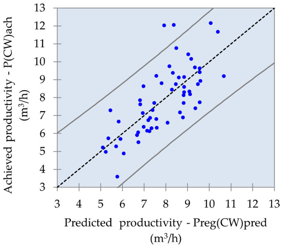
Figure 1.
Agreement of achieved and predicted productivity–regression model.
5. Simulation Model
In the following text, a description of the preparation and creation of the simulation model for predicting the productivity is given. For the needs of this part of the paper—formation of the simulation model—the data collected on the construction sites are statistically processed using the XLSTAT 2014 add-on of Excel. After testing the samples for the presence of outliers using the Grubb’s test for outliers, based on Expressions (2) and (3), statistical analysis and corresponding probability distributions are provided. All the obtained probability distributions are presented as values of the corresponding parameters in the model that were used independently or for forming of corresponding functions, or the distribution parameters are used directly for the presentation of the duration of individual processes and operations.
5.1. Data Preparation for Creating the Simulation Model
Preparation of input data for the simulation model involves a statistical analysis of the collected data and the determination of the appropriate probability distribution functions. The values of some parameters in the model that were used to create model functions or to represent the duration of specific processes and operations are expressed as random variable functions of specific probability distributions.
The mathematical expressions of the used probability distribution functions (5–7) are shown below.
Beta4 probability distribution function is used for the mixer movement speed when transporting concrete to the construction site. Data on the duration of concrete transport from the concrete factory to the construction site, collected by recording the process, are divided into two groups depending on the transport route: transport through the city and transport outside the city. It was observed that different mean speeds were achieved for these two modes; lower speeds were achieved, of course, in the first case, due to the effects of traffic lights, intersections, city congestion, etc. Based on the distance of the appropriate concrete factory from the observed construction site and the achieved transport time, the movement speeds of the mixer were calculated, sorted in relation to the transport route, and the corresponding theoretical probability distribution functions were obtained.
For the transport of concrete to the construction site in the case of city driving, it was found that the speed of movement is best represented by the Beta4 distribution function, which is given by the density function [33]:
where a, b (a > 0, b > 0) are shape parameters and c, d (c, d ∈ R, c < d) are the lowest and highest values of the random variable.
The Beta4 function is used to describe various phenomena characterized by random variables with values that are in a finite interval.
The zero hypothesis was tested: the considered empirical distribution has the features of the Beta4 distribution and the alternative hypothesis, considered empirical distribution, does not have the Beta4 characteristics. Based on the Kolmogorov–Smirnov test, since the p-value 0.834 is considerably greater than α = 0.05, the zero hypothesis at the reliability level of 95% is adopted. The risk for rejection of the zero hypothesis, if correct, is 83.36%. In Table 5 are provided the Beta4 distribution parameters for the realized movement speed.
Table 5.
Probability distributions for the simulation model.
For the case of extra-urban driving, it was found that the speed of movement is best represented, also by the Beta4 distribution function, with slightly different parameter values (Table 5).
Recorded times of mixer unloading are reduced to the unloading time in minutes per cubic meter of unloaded and placed concrete. In this way, the probability distribution function is obtained for concreting of columns and walls in Weibull (3) (Table 5).
Weibull (3) probability distribution function [33]:
where a (a > 0) is the shape parameter, b (b > 0) is the scale parameter, and c (c ∈ R) is the location the parameter.
The time required for positioning (parking) the mixer in the position for unloading concrete into the pump hopper is represented by appropriate probability distributions depending on the parking approach: parking within the construction site and parking from the street. On the construction site, space is generally provided for the unhindered movement of the mixer during positioning. On the other hand, if the space of the construction site is narrow and the position of the building is such that the pump is located on the street or sidewalk, it is also necessary for the mixer to be on the street, and its maneuvering and placing in the appropriate position will depend on the current traffic situation (waiting for the passage of vehicles and pedestrians, etc.). All measured mixer positioning times were divided into two groups depending on the approach, and different probability distribution functions were obtained. For the positioning of the mixer inside the construction site, the time is represented by the function Weibull (3) (Table 5).
After the concrete has been unloaded at the construction site, the mixer hopper is washed with water. For the case of hopper washing, the best agreement with the function Weibull (3) was obtained (Table 5).
Log-normal probability distribution function [33]:
where m (m ∈ R) is the shape parameter, σ (σ > 0) is the scale parameter.
The proposed independent variables for the simulation model are the same as in the regression model. Since the simulation model is a dynamic system, its creation necessitated the introduction of the duration of specific operations. Table 5 shows the operations introduced in the simulation model expressed using their corresponding probability distributions with distribution parameters.
5.2. Creation of the Simulation Model
The simulation model was created using AnyLogic modeling software, which is based on the Java object-oriented interface. The software is able to create a model by combining different simulation methods, discrete event simulation (DES), system dynamics (SD), and agent-based modeling (ABM), and by creating hybrid multimethods [34]. In the present study, a hybrid method was used to create the simulation model of the concreting process—a combination of DES and ABM. The simulation model was created by connecting different blocks that represent specific operations during the concreting process. There is a great variety of blocks in the software library, and they are connected via connectors. Depending on the type, each block comprises the necessary properties, such as agent name, agent type, duration, capacity, maximum capacity, agent location, agent actions at different moments in time (e.g., at the entrance or exit), etc. Each block is assigned a function or parameters that describe a given operation. In addition to process diagrams representing the concreting process, state charts were also used to represent the behaviors of specific parts of the system (Figure 2).

Figure 2.
Concreting process diagram with state charts–simulation model.
Before running the simulation, it is necessary to define the input variables and parameters by selecting the available options and entering the values for parameters such as concrete amount, number of elements, number of workers, etc. For this purpose, a window for entering input data appears prior to the running of the simulation (Figure 3).
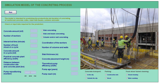
Figure 3.
Definition of input parameters before running the simulation.
The application provides different representations of the simulation model—logical (Figure 2) as well as 2D (Figure 4a) and 3D (Figure 4b).

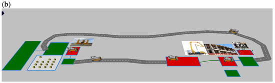
Figure 4.
Representations of the simulation model: (a) 2D; (b) 3D.
It is possible to view the changes of various states, quantities, and parameters during the simulation from a number of diagrams, histograms, and variables (Figure 5).
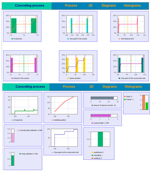
Figure 5.
Changes in the state of the system during simulation.
6. Analysis and Comparison of the Models
The models were verified, analyzed, and compared based on the mean absolute percentage error (MAPE) and the absolute percentage error (APE). According to [35], MAPE and APE are shown by the following expressions:
MAPE was 13.27% for the regression model and 21.99% for the simulation model. Figure 6 shows the comparison of the predicted productivity from both models and the achieved productivity.
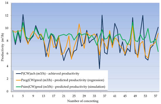
Figure 6.
Agreement of achieved productivity with predicted productivity (regression and simulation).
The comparative evaluation of the proposed models was performed through a comparison of the achieved productivity with the productivities predicted using the regression model, specifically Expression (2), and the simulation model, based on simulation experiments. To obtain simulation output data, experiments were conducted for all the cases recorded at the construction site. Depending on the scattering of the results, the required number of simulations was computed, and 20 simulations were run for every concreting, so 1160 simulations in total, with different strings of random numbers because of the presence of random variables [11].
The simulation model did not produce better results than the regression model because the concrete plant availability was not included as a parameter when it was created. In the seven cases when the concrete plant was busy supplying concrete to other construction sites, there was a significantly longer pump waiting time, which in turn led to stoppages, extended duration, and reduced productivity. The regression model clearly demonstrates the significance of this variable, by the regression coefficient of −1.933. When creating the simulation model, it was not possible to consider the concrete plant’s availability, because the process at the concrete plant was not recorded, and, thus, there were no precise data to be introduced into the simulation. In the regression model, this influence was expressed via two simple options: concrete plant is available (produces concrete for the analyzed construction site only) and concrete plant is not fully available (produces concrete for other purposes as well).
To evaluate the proposed models, the absolute percentage errors were divided into the following groups: up to 10%, 10–25%, 25–50%, and over 50%. Figure 7 shows the comparison of the results for both models in relation to the set groups of errors.
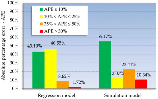
Figure 7.
Absolute errors of predicted values for the regression and the simulation model.
A higher percentage of simulation results was obtained with up to 10% error, around 55% of all productivities, whereas, in the regression model, around 43% fall within this group. On the other hand, around 90% of all regression model results were obtained with an error up to 25%, while the simulation yielded only 67% of its results within this group. A major error exceeding 50% occurred with only one regression result, as opposed to over 10% of the simulation results. The major errors in the simulation results occurred exactly for those measurements when the concrete plant was busy and concrete was not delivered on time. Therefore, the simulation was checked for the cases when the concrete plant was fully available. To that end, simulations were run on a reduced sample of 51 concreting tasks [11]. The same number of simulations were run as for the complete sample, and the obtained MAPE was 14.30%, which is less than the first case and almost the same as in the regression. Individual percentage errors by error group for this sample are shown in Figure 8.
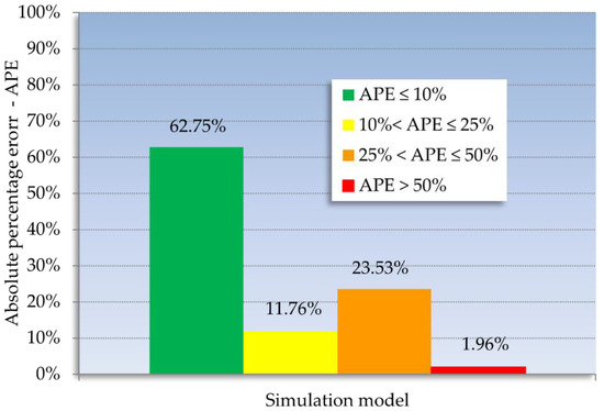
Figure 8.
Absolute errors of predicted values of the simulation model for the case of full concrete plant availability.
Around 75% of all results are now below the 25% absolute error boundary, but there are still many results (23.53%) with errors between 25% and 50%. To explain this phenomenon, an analysis was performed based on the following adopted productivity ranges: less than 7 m3/h, between 7 m3/h and 10 m3/h, and more than 10 m3/h. Figure 9 shows the obtained errors for every productivity group for each model.
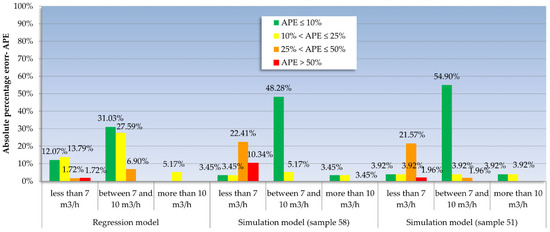
Figure 9.
Predicted value errors for the regression and the simulation model, according to productivity groups.
The comparison shows that the regression model produces better predictions for the productivity range between 7 and 10 m3/h, with most predicted value errors up to 25%. For the same range, the simulation model yielded around half of the results below a 10% error when concrete plant availability was considered, and around 55% of the results below a 10% error when plant availability was not considered. However, simulation predictions for productivity less than 7 m3/h are considerably less reliable, as most errors exceed 25%.
The data suggest that the regression model produces satisfactory productivity predictions with errors not exceeding 25% for any productivity range, regardless of whether the plant supplies only the analyzed construction site or not. On the other hand, the simulation model produces better predictions only when the plant supplies the analyzed construction site and no others, or when the plant supplied other sites simultaneously but without any interruptions to the analyzed construction site supply. The simulation model also produces better predictions for the productivity range between 7 and 10 m3/h, which is due to the adopted functions that represent parameters and variables.
7. Testing of the Proposed Models
The proposed models were tested on a case study of a building with five levels, where 12 concreting processes were recorded, from the basement to the fourth floor. The data were collected in the same manner as during the creation of the models, and the predicted productivity values were obtained using Expression (2) to test the regression model and using the simulation to test the simulation model. The mean measured productivity P(CW)achv was 8.27 m3/h, and the mean predicted productivity using regression Preg(CW)pred was 9.34 m3/h, which falls within the calculated regression MSE of 1.855 m3/h. The regression model testing resulted in MAPE of 15.05%.
Out of the 12 concreting processes, there were 2 where the concrete supply was delayed due to plant unavailability, so the simulation testing was conducted on a sample of 10 processes. The simulation produced the mean value of predicted productivities Psim(CW)pred of 9.13 m3/h and MAPE of 10.39%. The simulation model had previously proved superior to the regression model for the productivity range between 7 and 10 m3/h, which was confirmed in this case study, as the mean error was smaller than in the regression test.
8. Conclusions
This paper presented two original models for predicting the productivity of reinforced column and wall concreting.
The regression model was created using the backward elimination of variables that were statistically insignificant and a model was developed in which four independent variables explain around 53% of productivity variability. Using the coefficient of determination, it was shown that a moderately strong connection exists between the dependent variable and the independent variables. The mean squared error of this model was 13.27% during the development and 15.05% after case study testing. Such statistical indicators, which are somewhat inadequate, may have been influenced by the fact that multiple different contractors were involved (a different one on each construction site) and that the sample size was relatively small. Likewise, the influence of the number of columns and walls in the sample was not the same. The regression model can be used to predict the productivity of the column and wall concreting, regardless of the value of the expected productivity and of whether the concrete plant serves other construction sites or not.
The simulation model was created using AnyLogic modeling software, which is based on the Java object-oriented interface, and applying discrete event simulation in conjunction with agent-based modeling. As opposed to the regression model, the simulation model contains all the variables, regardless of their statistical significance, owing to the very nature of its operation as a dynamic system. This model not only has better predictive power (with an error up to 10%) but also has a restriction that it can only be used in cases when a concrete plant does not simultaneously supply concrete to other construction sites and for the expected productivity ranges between 7 and 10 m3/h. Nevertheless, the simulation model proved to be superior based on the mean error of 10.39% after testing.
One of the important factors for the successful implementation of a construction project is the good planning of the works to achieve the highest possible productivity on the construction site.
The findings obtained from this study would:
- Provide a better understanding of concreting process productivity;
- Identify significant influencing factors on the productivity in certain conditions;
- Show how to achieve a better productivity.
When concreting columns and walls, the characteristics of the work crew have a significant impact on productivity.
The proposed models can be useful in the planning phase and enable more accurate forecasting of the duration of activities during the performance of concrete works and, thus, usefully influence decision-making, forecasting the flow of works, and better management of the concreting process, with the aim of increasing productivity, shortening duration, and reducing costs.
The formed regression and simulation models can be a useful tool to help managers and engineers on the construction site plan the execution of works. These models, with quite a sufficient accuracy, provide a relatively quick prediction of the productivity and duration of the concreting process of certain elements.
The results of this study could be useful for the planning of important work activities, such as concreting. Adequate and realistic planning and prediction of productivity and, consequently, the duration of concreting can optimize the management of building construction.
The proposed prediction method of the productivity of the column and wall concreting process has certain limitations. The prediction results may have same errors due to uncertain factors such as construction environment, construction technology, and equipment. So, the developed model is proposed for application in similar conditions, and it then gives a satisfactory accuracy for the results.
Further research should be focused on expanding the database, studying the productivity of column and wall concreting using cranes for concrete transport, which is a frequently implemented technology, and applying other prediction methods.
Author Contributions
Conceptualization, B.M.-N.; methodology, B.M.-N.; software, B.M.-N.; validation, B.M.-N. and L.Ž.; formal analysis, B.M.-N.; investigation, B.M.-N.; resources, B.M.-N.; data curation, B.M.-N.; writing—original draft preparation, B.M.-N.; writing—review and editing, B.M.-N. and L.Ž.; visualization, B.M.-N. and L.Ž.; supervision, L.Ž.; project administration, B.M.-N. All authors have read and agreed to the published version of the manuscript.
Funding
This research received no external funding.
Data Availability Statement
No applicable.
Conflicts of Interest
The authors declare no conflict of interest.
References
- Motyčka, V.; Gašparík, J.; Přibyl, O.; Štěrba, M.; Hořínková, D.; Kantová, R. Effective use of tower Cranes over time in the selected construction process. Buildings 2022, 12, 436. [Google Scholar] [CrossRef]
- Alaloul, W.S.; Alzubi, K.M.; Malkawi, A.B.; Salaheen, M.A.; Musarat, M.A. Productivity monitoring in building construction projects: A systematic review. Eng. Construct. Arch. Manag. 2022, 29, 2760–2785. [Google Scholar] [CrossRef]
- Maqsoom, A.; Aslam, B.; Gul, M.E.; Ullah, F.; Kouzani, A.Z.; Mahmud, M.P.; Nawaz, A. Using multivariate regression and ANN models to predict properties of concrete cured under hot weather. Sustainability 2021, 13, 10164. [Google Scholar] [CrossRef]
- Bisták, A.; Hulínová, Z.; Neštiak, M.; Chamulová, B. Simulation modeling of aerial work completed by helicopters in the construction industry focused on weather conditions. Sustainability 2021, 13, 13671. [Google Scholar] [CrossRef]
- Terzioglu, T.; Polat, G.; Turkoglu, H. Formwork System Selection Criteria for Building Construction Projects: A Structural Equation Modelling Approach. Buildings 2022, 12, 204. [Google Scholar] [CrossRef]
- Terzioglu, T.; Polat, G. Formwork System Selection in Building Construction Projects Using an Integrated Rough AHP-EDAS Approach: A Case Study. Buildings 2022, 12, 1084. [Google Scholar] [CrossRef]
- Terzioglu, T.; Polat, G.; Turkoglu, H. Analysis of industrial formwork systems supply chain using value stream mapping. J. Eng. Proj. Prod. Manag. 2022, 12, 47–61. [Google Scholar] [CrossRef]
- Lee, B.; Choi, H.; Min, B.; Ryu, J.; Lee, D.E. Development of formwork automation design software for improving construction productivity. Autom. Constr. 2021, 126, 103680. [Google Scholar] [CrossRef]
- Ma, W. Behavior of Aged Reinforced Concrete Columns under High Sustained Concentric and Eccentric Loads. Doctoral Dissertation, University of Nevada, Las Vegas, NV, USA, 2021. Available online: https://digitalscholarship.unlv.edu/cgi/viewcontent.cgi?article=5178&context=thesesdissertations (accessed on 15 October 2022).
- Matejevic, B.; Zlatanovic, M. Regression model for predicting productivity of RC slab concreting process. Gradjevinar 2017, 69, 561–572. [Google Scholar] [CrossRef]
- Matejevic, B. Model za Prognoziranje Produktivnosti Procesa Betoniranja (Model for Predicting of the Productivity of the Poncreting Process). Ph.D. Thesis, The Faculty of Civil Engineering and Architecture, University of Nis, Nis, Serbia, 2016. Available online: https://nardus.mpn.gov.rs/handle/123456789/8285 (accessed on 25 April 2020). (In Serbian).
- Dunlop, P.; Smith, S.D. Estimating key characteristics of the concrete delivery and placement process using linear regression analysis. Civ. Eng. Environ. Syst. 2003, 20, 273–290. [Google Scholar] [CrossRef]
- Dhawale1, A.W.; Nizamuddin, K.R. Concrete Productivity and Performance Comparison of Pumped Concrete for High Rise Structure. Int. J. Rec. Innov. Trends Comput. Commun. 2016, 4, 77–79. [Google Scholar]
- Panas, A.; Pantouvakis, J.P. Multi-attribute regression analysis for concrete pavement productivity estimation. Organ. Technol. Manag. Construct. Int. J. 2011, 3, 289–295. [Google Scholar] [CrossRef][Green Version]
- Olaoluwa, O.; Adesanya, D.A. Productivity of Concrete Placement by Dumpers in Nigeria. Int. J. Eng. Res. Dev. 2015, 11, 15–28. Available online: http://www.ijerd.com/paper/vol11-issue3/Version_1/C1131528.pdf (accessed on 19 March 2021).
- Karthick, R. A study on productivity of concreting work in building construction in Bengaluru city, India. Int. Res. J. Eng. Technol. (IRJET) 2018, 5, 1604–1609. [Google Scholar]
- Aparna, B.; Kuriakose, L.T. Influential Factors Affecting Labour Productivity in Concreting of Columns. Int. J. Innov. Eng. Technol. (IRIET) 2015, 5, 71–77. [Google Scholar]
- Jarkas, A.M. Buildability factors influencing concreting labor productivity. J. Construct. Eng. Manag. 2012, 138, 89–97. [Google Scholar] [CrossRef]
- Abd-El, H. Predicting the Production Rate of Pouring Ready Mixed Concrete Using Regression Analysis. J. Civ. Eng. Sci. 2014, 3, 219–234. Available online: https://kipdf.com/predicting-the-production-rate-of-pouring-ready-mixed-concrete-using-regression-_5afe5c8f8ead0eb0158b461b.html (accessed on 25 April 2020).
- Han, S.; Hao, P. Lessons learned from schedule estimation using real-time data in a concreting operation. In Proceedings of the 28th ISARC, Seoul, Korea, 29 June–2 July 2011; pp. 886–891. [Google Scholar] [CrossRef]
- Park, M.; Kim, W.-Y.; Lee, H.-S.; Han, S. Supply chain management model for ready mixed concrete. Autom. Construct. 2011, 20, 44–55. [Google Scholar] [CrossRef]
- Matejevic, B.; Zlatanovic, M.; Cvetkovic, D. The Simulation Model for Predicting the Productivity of the Reinforced Concrete Slabs Concreting Process. Tech. Gaz. 2018, 25, 1672–1679. [Google Scholar] [CrossRef]
- Lu, M.; Anson, M.; Tang, S.L.; Ying, Y.C. HKCONSIM: A practical simulation solution to planning concrete plant operations in Hong Kong. J. Construct. Eng. Manag. 2003, 129, 547–554. [Google Scholar] [CrossRef]
- Lu, M.; Lam, H.C. Optimized concrete delivery scheduling using combined simulation and genetic algorithms. In Proceedings of the Winter Simulation Conference, Orlando, FL, USA, 4–7 December 2005. [Google Scholar] [CrossRef]
- Hassan, M.M.; Gruber, S. Estimation of concrete paving construction productivity using discrete event simulation. In Proceedings of the 43th Annual Conference of the Associated Schools of Construction, Flagstaff, AZ, USA, 12–14 April 2007; Available online: http://ascpro0.ascweb.org/archives/cd/2007/paper/CPRT86002007.pdf (accessed on 18 September 2021).
- Talian, J. Optimization of the concrete delivery and placement process using a simulation. Slovak J. Civ. Eng. 2013, 21, 1–6. [Google Scholar] [CrossRef]
- Zayed, T.M.; Halpin, D. Simulation of concrete batch plant production. J. Construct. Eng. Manag. 2001, 127, 132–141. [Google Scholar] [CrossRef]
- Tahmasebinia, F.; Jiang, R.; Sepasgozar, S.; Wei, J.; Ding, Y.; Ma, H. Implementation of BIM energy analysis and monte carlo simulation for estimating building energy performance based on regression approach: A case study. Buildings 2022, 12, 449. [Google Scholar] [CrossRef]
- Mendenhall, W.; Sincich, T. A Second Course in Statistics: Regression Analysis, 7th ed.; Pearson: New York, NY, USA, 2011; pp. 168–182. Available online: https://www.pearsonhighered.com/assets/preface/0/1/3/5/013516379X.pdf (accessed on 1 September 2022).
- Grubbs’ Test for Outliers. Available online: https://www.itl.nist.gov/div898/handbook/eda/section3/eda35h1.htm (accessed on 15 October 2022).
- Statistical Tables. Available online: https://home.ubalt.edu/ntsbarsh/Business-stat/StatistialTables.pdf (accessed on 15 April 2020).
- Chicco, D.; Warrens, M.J.; Jurman, G. The coefficient of determination R-squared is more informative than SMAPE, MAE, MAPE, MSE and RMSE in regression analysis evaluation. PeerJ Comput. Sci. 2021, 7, e623. [Google Scholar] [CrossRef] [PubMed]
- Đorić, D.; Jevremović, V.; Mališić, J.; Nikolić-Đorić, E. Atlas Raspodela (Atlas of Distribution), 1st ed.; Građevinski Fakultet: Beograd, Serbia, 2007; pp. 30–247. Available online: http://poincare.matf.bg.ac.rs/~v_jevremovic/atlas.pdf (accessed on 10 June 2021).
- AnyLogic Multimethod Simulation Software. Available online: https://www.anylogic.com (accessed on 22 June 2020).
- Peško, I. Model for Estimating the Cost and Duration of Construction of Urban Road. Doctoral Dissertation, University of Novi Sad, Novi Sad, Serbia, 2013. Available online: https://www.yumpu.com/xx/document/view/21550879/model-za-procenu-troskova-i-vremena-izgradnje-gradskih (accessed on 15 October 2022).
Publisher’s Note: MDPI stays neutral with regard to jurisdictional claims in published maps and institutional affiliations. |
© 2022 by the authors. Licensee MDPI, Basel, Switzerland. This article is an open access article distributed under the terms and conditions of the Creative Commons Attribution (CC BY) license (https://creativecommons.org/licenses/by/4.0/).