Article

Deep Learning-Enriched Stress Level Identification of Pretensioned Rods via Guided Wave Approaches

1
Department of Civil and Environmental Engineering, North Dakota State University, Fargo, ND 58018, USA
2
School of Civil Engineering, Dalian University of Technology, Dalian 116024, China
*
Author to whom correspondence should be addressed.
Buildings 2022, 12(11), 1772; https://doi.org/10.3390/buildings12111772
Submission received: 24 September 2022 / Revised: 16 October 2022 / Accepted: 20 October 2022 / Published: 22 October 2022

Abstract

:
By introducing pre-compression/inverse moment through prestressing tendons or rods, prestressed concrete (PC) structures could overcome conventional concrete weakness in tension, and thus, these tendons or rods are widely accepted in a variety of large-scale, long-span structures. Unfortunately, prestressing tendons or rods embedded in concrete are vulnerable to degradation due to corrosion. These embedded members are mostly inaccessible for visual or direct destructive assessments, posing challenges in determining the prestressing level and any corrosion-induced damage. As such, ultrasonic guided waves, as one of the non-destructive examination methods, could provide a solution to monitor and assess the health state of embedded prestressing tendons or rods. The complexity of the guided wave propagation and scattering in nature, as well as high variances stemming from the structural uncertainty and noise interference PC structures may experience under complicated operational and harsh environmental conditions, often make traditional physics-based methods invalid. Alternatively, the emerging machine learning approaches have potential for processing the guided wave signals with better capability of decoding structural uncertainty and noise. Therefore, this study aimed to tackle stress level prediction and the rod embedded conditions of prestressed rods in PC structures through guided waves. A deep learning approach, convolutional neural network (CNN), was used to process the guided wave dataset. CNN-based prestress level prediction and embedding condition identification of rods were established by the ultrasonic guided wave technique. A total of fifteen scenarios were designed to address the effectiveness of the stress level prediction under different noise levels and grout materials. The results demonstrate that the deep learning approaches exhibited high accuracy for prestressing level prediction under structural uncertainty due to the varying surrounding grout materials. With different grout materials, accuracy could reach up to 100% under the noise level of 90 dB, and still maintain the acceptable range of 75% when the noise level was as high as 70 dB. Moreover, the t-distributed stochastic neighbor embedding technology was utilized to visualize the feature maps obtained by the CNN and illustrated the correlation among different categories. The results also revealed that the proposed CNN model exhibited robustness with high accuracy for processing the data even under high noise interference.

1. Introduction

Conventional reinforced concrete, due to the weakness of the concrete in tension, often shows cracking and corrosion at an early age [1,2]. PC has been proposed through prestressing/post-tensioning tendons/rods to compensate this drawback [3]. PC structures exhibit dramatically improved performance over conventional reinforced concrete ones, with the contribution of prestressing tendons or rods that enable them to cover a longer span, thereby providing an effective solution in large-scale buildings, bridges, dams, and nuclear power plant structures. It is known that PC structures often experience losses in prestress due to various factors, including shrinkage/creep of concrete and relaxation of tendons/rods, which in turn potentially lead to excessive deflection or cracking. As such, being able to quantify the stress level of these prestressing tendons/rods in service conditions is critical to ensure structural integrity and achieve successful performance. However, conventional visual or direct destructive examination tools are not valid, as the embedded prestressing tendons or rods with or without grout materials are often inaccessible. Therefore, non-destructive examination (NDE) methods and tools, including vibration-based sensors [4], distributed sensors [5], ultrasonic guided waves [6,7], or acoustic emission [8], could capture information of those far-reaching, inaccessible locations, while maintaining high-quality monitoring and assessing of structural health. For instance, Bartoli et al. [4] employed dynamic identification techniques to investigate the correlation between PC beam prestressing forces. Their results demonstrated that the vibration frequency could assist in identifying the prestress level. Chen et al. [5] used distributed sensor, long-gauge fiber Bragg grating to detect the damage of a bridge under stochastic traffic flow. In addition, the existence of anomalies is an important issue in monitoring data; hence, Zhang et al. [9] employed Bayesian dynamic regression to reconstruct missing data. Despite the merits of different sensing techniques, vibration-based methods are often limited in low frequency, while distributed sensors are often vulnerable to damage and anomalies. Alternatively, as stated in the literature [6,10,11,12,13], ultrasonic guided waves could be a better solution to tackle such situations, with the advantages of far-reaching, long-distance measurement and high accuracy in detecting small changes in material discontinuity. Additionally, as an active method, ultrasonic guided wave testing can judge the sensitivity and accuracy of a sensor by receiving the excitations, reducing the possibility of receiving abnormal data.
Guided waves are widely used to evaluate the health of beams, plates, and pipes, owing to the potential of long-distance propagation and sensitivity to mechanical damage. Three modes, namely longitudinal, flexural, and torsional modes, are generated when guided waves are propagated in a medium. Among them, longitudinal modes are more sensitive to tensile stress and easy to excite by piezoelectric actuators [14], and are used for the inspection of steel bars for corrosion, fracture, and stress reduction. Bread et al. [10] used the pulse-echo technique to detect the corrosion and fracture of grouted tendon anchors and rock bolts by ultrasonic guided waves. Lanza di Scalea et al. [15] applied guided waves through magnetostrictive transducers to monitor the stress in seven-wire strands. Their results demonstrated the feasibility of determining the prestress level using the guided wave method. Ervin et al. [16] created an embeddable ultrasonic sensor network to localize and monitor the corrosion of rebar embedded by mortar. They studied the characteristics of guided wave propagated in rebar and the effect forms for corrosion detection, and showed that the waves were sensitive to corrosion through scattering, mode conversions, and reflections. Chaki and Bourse [17] detected the stress level of the seven-wire steel strands by ultrasonic guided waves with L (0,1) mode. The typical calibration curves were plotted, which showed that the stress level corresponded to the phase velocity change in the guided waves. More recently, Treyssède and Laguerre [18] employed the semi-analytical finite element approach to study the guided wave propagation in multi-wire strands. In addition, high-order longitudinal modes were indicated to solve the leakage problem of fundamental mode L (0,1) by Dubuc et al. [19]. They used the acoustoelastic theory to propose an approximate theory for predicting the effect of stress on higher modes. Shoji Masanari [20] employed 60 kHz L (0,1) mode as the guided wave to inspect anchor rods embedded in soil, and unveiled the capability of the ultrasonic guided waves for stress identification in rods. While physics-based approaches have been used for the signal process of guided waves to identify stress changes in stressed rods, these methods still face challenges in handling the wave signals with a variety of structural uncertainties, signal attenuation, and environmental noises during testing.
In this way, recently emerging machine learning, particularly deep learning, could provide potential solutions to improve the signal process of guided waves [6,7,21,22]. Deep learning algorithms have been employed in time series [21,23,24,25,26] and image processing [27,28,29,30]. Guo et al. [31] utilized a sparse coding-based deep learning algorithm to process wireless sensory data of a three-span bridge. The features of the dataset were learned by sparse coding and then trained by the network. Cha et al. [27] proposed a vision-based method by a deep learning network to detect concrete cracks without calculating the features. The comparative study indicated that the deep learning-based technique had better performance than the conventional physics-based methods. Furthermore, Cha et al. [28] investigated the fast region-based convolutional neural network to detect five types of damage in real time. Zhang et al. [32] proposed a CNN framework with some convolutional kernels to identify vibration signals. Harsh et al. [33] applied high-frequency guided waves to detect damages in railheads, generated the data by experiment and simulation study, and then set up a framework to detect damage of railheads by a machine learning method. The error rate was from 2% to 16.67%. Tabian et al. [34] used guided waves to detect impact energy, localization, and characterization of complex composite structures. The waves transferred into 2D images and were identified by a CNN algorithm. The results showed that the accuracy was above 95%. Zargar and Yuan [35] used a unified CNN-RNN network to extract the information of aluminum plates. This research focused on the wave propagation in both spatial and temporal domains. While deep learning approaches have been successfully used in many aspects of structural health monitoring, less research is involved in deep learning-based ultrasonic guided wave diagnoses.
Therefore, we aimed to develop and implement the deep learning-enriched guided wave technique to quantify the stress level of prestressed rods used in PC structures. The CNN framework was utilized for processing guided wave signals to predict the stress level of the rods with varying grout materials. t-distributed stochastic neighbor embedding (t-SNE) was employed to visualize the features extracted by the CNN model. Moreover, different noise levels were considered to examine the robustness of the CNN classifier.

2. Guided Waves as NDE Approach for Prestressed Rods

2.1. Governing Equations and Simulation of Guided Waves along a Rod

Guided waves were first introduced in cylinder structures in the 19th century [36]. The governing equation of the wave propagating in isotropic cylinders is expressed as [37]
( λ + 2 μ ) ( u ) + μ 2 u + f = ρ ( 2 u x 2 )
where u represents the displacement vector, x is the time, 2 is the three-dimensional Laplace operator, λ and μ indicate Lame’s constants, ρ is the mass density, and the body force f is equal to zero. Then, the Helmholtz decomposition is used in Equation (1) to simplify the problem as
u = φ + H
H = 0
where φ and H represent the scalar and vector potentials.
Three types of guided waves, namely longitudinal mode (L (0, m)), torsional mode (T (0, m)), and flexural mode (F (n, m)), were generated to propagate through a cylindrical structure. In the modes, n and m denote the circumferential order and modulus, respectively. When n = 0, the waves are symmetrical, such as L (0, m) and T (0, m). Otherwise, the waves are asymmetrical.
Stress affects the phase velocity of the guided wave. The change in the phase velocity Δ C is expressed as
Δ C = [ ( C 0 ) 2 l ] Δ t
where C 0 is the unstressed velocity, l represents the length of the wave propagation in the stress area, and Δ t is the time change.
Figure 1 shows the phase velocity and group velocity derived by MATLAB PCDisp [38,39]. The lower frequency of the excitation waves, less than 50 kHz, was used to reduce the dispersion of the guided waves.
As such, the ultrasonic guided waves used in this study were numerically simulated by Multiphysics Finite Element (FE) software COMSOL, and their propagation characteristics along the prestressed rod under different conditions, including under varying grout materials and different stress levels, were then modeled and extracted using machine learning to assist in data classification, as discussed in Section 3.

2.2. Calibration of the FE Analysis of the Ultrasonic Guided Waves through the Rod

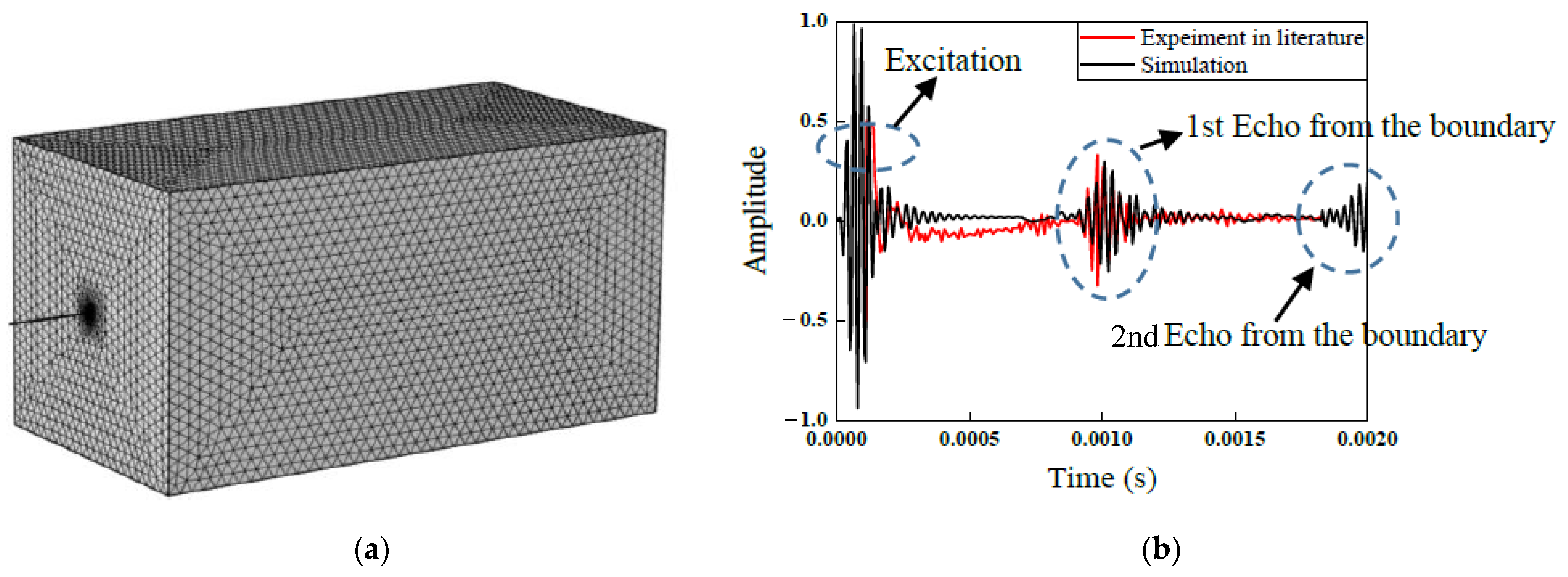
We sought to ensure that proper parameters were used for the rod simulation and calibrate the effectiveness of FE-based simulation for capturing the characteristics of the wave propagation along rods. One case of the characterization of ultrasonic guided waves along an anchor rod was selected from the literature [40], in which the rod had a diameter of 21 mm and was 2.3 m in length, and was embedded in a concrete block with a cross-section of 1.0 m by 1.0 m and a depth of 2.0 m, as shown in the FE meshed model in Figure 2a. The excitation of the ultrasonic guided waves was a six-cycle tone burst with a frequency of 35 kHz. A pulse-echo test was set up on the rod where the actuators and receivers were on the same side. Excitations were generated by Wavemaker 16 equipment, which is used for long-range inspection of pipes. The rod was embedded in the concrete block along 2 m and the remaining length of the rod from both ends of the block [40]. The comparison results are shown in Figure 2b, where signals in the literature are marked with red lines and the black ones were generated from this study, and the three circled wave packets denote the excitation signals, the first right boundary reflection, and the second right boundary reflection. As shown in Figure 2b, the simulated guided waves in this study matched well with the experimental data collected from the literature in most cases, where three wave packets were captured well. The first boundary wave reflections from simulated signals occurred at 0.001 s, identical to the experimental data with comparable amplitudes. Note that some deviations occurred after the excitation, and a potential reason could partially result from the attenuation of the concrete block where the simulation did not capture well. However, the entire trend and amplitudes in most cases were in agreement with the literature, suggesting that the simulation used in this study was appropriate to ensure capturing of the characteristics of the ultrasonic guided waves through the rods.

2.3. Design of Scenarios

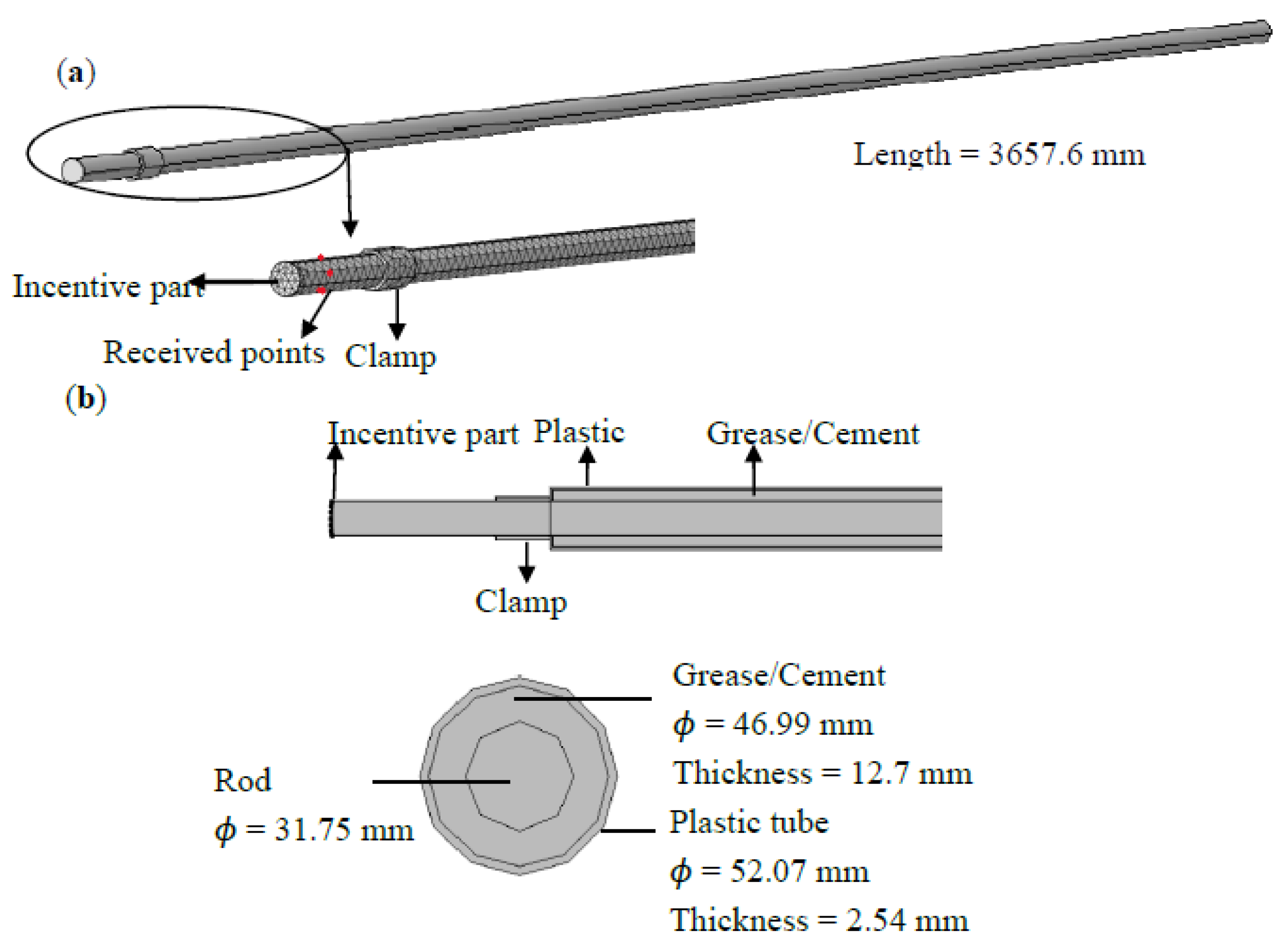
Followed by the calibration in Section 2.2, this section details the design of different scenarios to generate datasets that helped to elucidate the critical factors affecting the characteristics of ultrasonic guided wave propagation along stressed rods, thus paving the way for stress level prediction using machine learning in Section 3. As such, the prototype of the stressed rods was derived from the literature [41]. The rod was 31.75 mm in diameter with a length of 3657.6 mm. The material properties of the rod were density of 7800 kg/m3, Young’s modulus of 2 × 10⁵ MPa, and Poisson ratio of 0.3. A clamp served as the anchorage of the rod, which was located 50.8 mm away from the free end. Besides the reference where the rod had no grout, two grout materials, namely grease and cement, were selected to unveil their effects on the effectiveness of the proposed methods. The density of the cement was 1440 kg/m3, the Young’s modulus was 2.5 × 10⁴ MPa, and the Poisson ratio was 0.25. The density of the grease was 2600 kg/m3. The detailed information of the rod models is shown in Figure 3. The entire rod with the clamp is illustrated in Figure 3a (note that the meshing figure is a schematic diagram; the actual meshing unit is much smaller), and the embedded rod is shown in Figure 3b. Specifically, the rod passed through the plastic pipe and then added grease and cement to fill the gap between the pipe and the rod. The outer diameter of the plastic pipe was 52.07 mm, and the thickness was 2.54 mm. In finite element studies, meshing is one of the critical parts in simulation. Free triangular element was selected in this model. Guided wave simulation requires a high-quality meshing system to minimize the propagation error of guided waves. Thus, a wavelength needs to contain at least eight elements. In this study, the maximum element size in the model was 2 mm and time steps were 5 × 10⁻⁶ s. Guided waves could be excited in the rod by adding displacement loads in all nodes of the left boundary in the model. The excitation waves were 35 kHz five-cycle sinusoidal waves modulated by the Hanning window. Four points, as received points, distributed the circumferential surface of the rod. Positions of received nodes were 5 mm away from the left side. Received signals were time series data, which intercept the first 1000 data points as results for further study.
To simulate the stress reduction in prestressed components, five different pressure levels were loaded into each rod: no prestress (State #1), 20% ultimate tensile strength (UTS) (State #2), 40% UTS (State #3), 60% UTS (State #4), and 80% UTS (State #5). In total, 15 cases were designed in this section, which are shown in Table 1. Noise was added into the data to increase the uncertainty of the dataset.

2.4. Data Collection and Augmentation

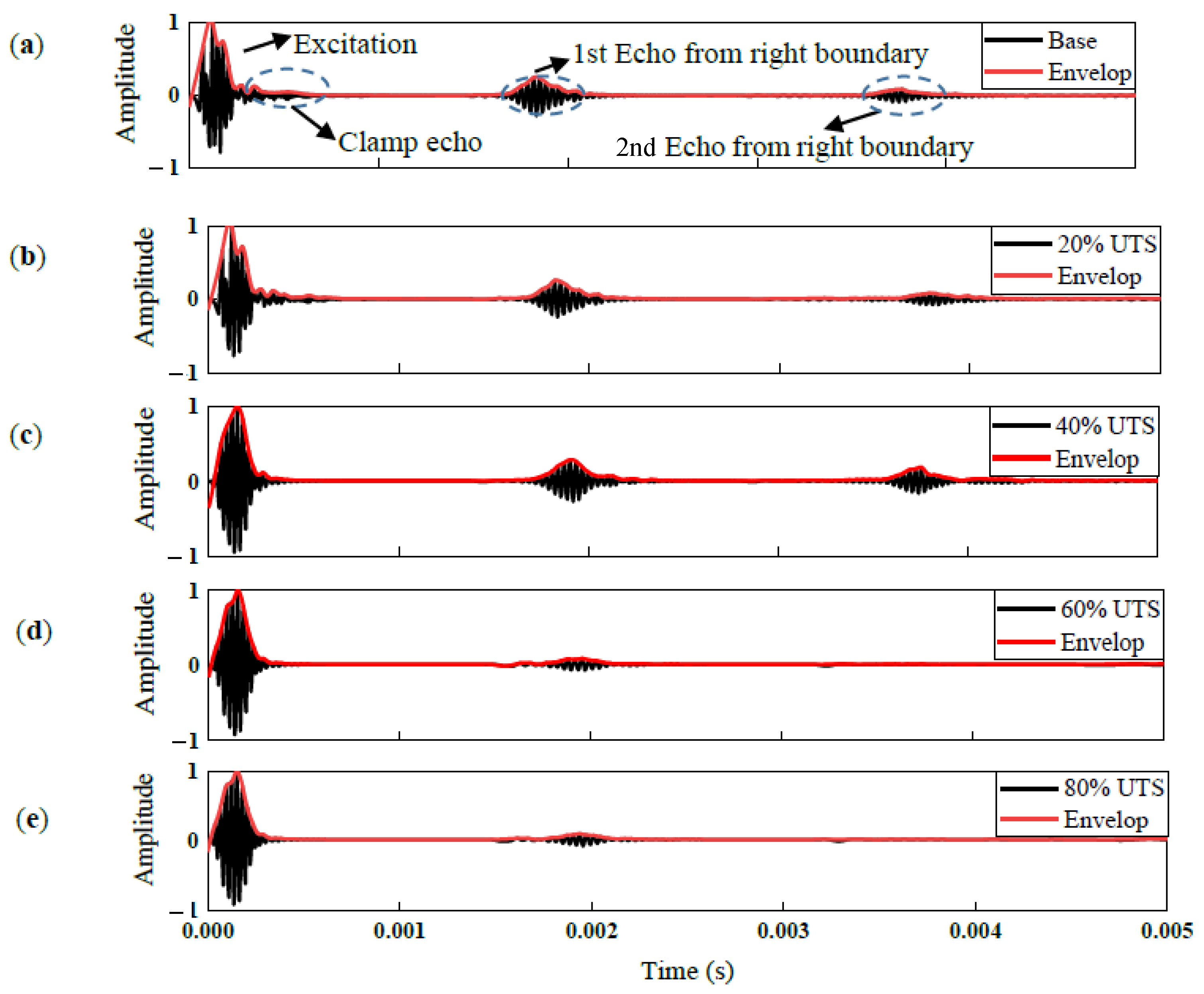
Figure 4 shows the time records with five different prestress levels derived from the finite element simulation in Case 1 from Table 1. The received point was located 5 mm away from the left side of the rod. To ensure the input wave had similar energy, all the received signals were normalized, and the maximum amplitude of the first packet was equal to 1. The time series were from 0 s to 0.005 s; the guided wave can propagate and reflect at least twice throughout the rod. Figure 4a–e illustrates the received signals of the steel with prestress levels equal to 0% UTS, 20% UTS, 40% UTS, 60% UTS, and 80% UTS. Specifically, at low prestress level states (0–40% UTS), the results clearly exhibit three main wave packets that represent the initial excitation and the first and second reflections from the boundary. Following the first packet, fluctuations with small amplitude were echoes from the clamp. With the stress level increased, the amplitude of this part was smaller, and it was hard to detect at 80% UTS. In addition, the velocity of guided waves reduced with increasing the stress of the rod. The first reflection from the right boundary was around 0.0018 s in the base state. The value was raised to 0.0019 s and 0.002 s when stresses were 40% UTS and 80% UTS. At 60% and 80% UTS (shown in Figure 4d,e), only two main packets existed in the signals, where one was initial input waves, and the other was the boundary reflection. The energy of guided waves was dissipated when waves propagated in the second cycle. Thus, it was difficult to detect the second echo from the boundary.
As illustrated in Figure 5, the collected guided waves of the rod exhibited different patterns from different grout materials. Figure 5 illustrates the signals collected from States #1, #6, and #11 (without stress) in the time domain and frequency domain. It was observed from the time domain that with long distance propagation, the energy of the reflection waves was reduced progressively. However, comparing these three states, the rod embedded in cement had the highest attenuation, where the peak value of reflections was reduced from 0.2588 to 0.1075. After propagating to the second cycle, the peak value of the second boundary echo was reduced to 0.0897 in the unembedded state, and the value of the rod in cement was the lowest, 0.0113. On the contrary, grease had less of an effect on guided waves. With 1463.04 mm of propagation, the peak value of the reflected waves was 0.0455, which was close to the unembedded state. In the frequency domain, it was clear that the main frequency of waves was 35 kHz. Some weak peaks occurred at the low frequency and the high frequency due to reflections from the clamp and the boundary.
A total of 15 states were designed to simulate the actual situation of the rod. In each state, four received nodes were distributed around the circumference and were located 5 mm away from the left side. Since the received waves were easily contaminated by noise, five noise levels based on the signal to noise ratio (SNR) were added into the received signals. In addition, noise involved in the signals could increase the uncertainties of the data, so we attempted to investigate the robustness of the deep learning methods. Figure 6 illustrates the collected signals at five different noise levels. When SNR exceeded 80 Db, the interference from noise was obvious and covered some original features of the initial signals. Especially, at 60 dB, the amplitude of the noise was greater than the signal amplitude, which was not conductive for further study.

3. Deep Learning Framework

CNN has been widely adopted in many application domains, such as image classification and segmentation, speech recognition, and computer vision tasks. The CNN framework contains multiple layers, including a convolutional layer, pooling layer, fully connected layer, and ReLU layer. These layers help to decode the input data into high-dimensional slices, extract the intricate features, and then encode them into the target values. In this study, CNN was used to identify the complicated guided wave signals. The architecture of the CNN trained by guided wave signals is described. The model of the CNN was changed from LeNet-5.

3.1. Introductions of CNN

The input data consisted of a series of signals with m detection points and n time steps. Thus, the size of the input layer was n × m.
The convolutional layer is one of the most crucial layers in a CNN. In this layer, each element from the kernel is multiplied with the data in the previous layer. The size of the kernel determines the operation area, and the number of kernels decides the third dimension of the output. The kernel size is much smaller than the input layer, so the kernel moves step by step to implement. The stride defines the length of each step, which causes the output data reduction. The size of the stride is an essential value which affects the efficiency and performance of the layer. A bigger size may cause the loss of some important features, and a small size may cause an increase in calculation. The initial kernels are generated randomly, and they update by learning from each iterator. A bias is added after summing all the multiplication results in the operation area. When all the kernels finish the multiplication with the input data and summarize, the result is the output in this layer.
The pooling layer is used to reduce the size of the previous layer. Two pooling layers can be selected, namely max pooling and mean pooling. In max pooling, the maximum values in the operation area are taken as the result. In mean pooling, the average values are the result. The operation area is also moved by setting the values of stride. After adding a pooling layer to a CNN framework, the output of the convolutional bands has a dramatic decrease. In this CNN, all the pooling layers were set as max pooling layers.
The activation layer adds nonlinearity into the CNN. In this model, ReLU was chosen as the activation layer in the CNN trained by guided wave signals. ReLU changes some of the neurons to zero, which will thin the network, reduce the interdependence between parameters, and avoid overfitting to some extent. In addition, it also saves computation and improves the efficiency of deep learning models, compared with other activation functions.
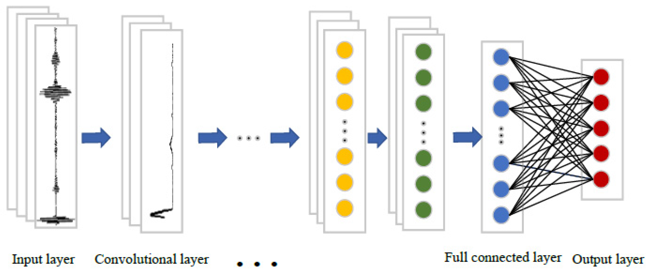
After the cooperation of several layers, the initial data are changed into a series of feature maps, and the size is deformed. To transfer these feature maps into their own category, a fully connected layer is necessary. The result of this layer is the probability that the data belong to each label. The entire process is shown in Figure 7.

3.2. CNN Architecture

The proposed CNN in this study was an eight-layer network, including three convolutional layers, two max pooling layers, a ReLU layer, a fully connected layer, and a softmax layer. The selection of hyperparameters affects the performance of the neural network. Different methods [27,42,43] have been proposed to select these parameters. For instance, the learning rate is to adjust the gradient update, the kernel number size is to adjust the receptive filed; in addition, stride step and batch size are critical in parameter design [26,41]. In this study, the hyperparameter selection stems from previous studies, maintaining the basic network architecture of LeNet-5. Note that several studies revealed that the introduction of Bayesian optimization [44,45] in determining the hyperparameters could further enhance the architecture of the CNN with less trial and error, and thus improve the accuracy. As part of the ongoing investigation of the applications of deep learning in civil structures, we consider advances in hyperparameter design, including using Bayesian optimization, for optimizing the CNN architecture.
The detailed information of each CNN layer is given in Table 2. The input data are a matrix sized 1000 × 4, representing four collected signals in a rod sample. A total of 1000 data points were intercepted from received signals, which included the excitation and the reflection from the right boundary. Four is the number of received signals. In the first convolutional layer, 20 filters sized 25 × 2 were generated and operated the input data into 976 × 3 × 20. The following was a max pooling layer with the stride equal to 5. The layer captured the maximum value in the response field and significantly cut down the size of the input. After that, the output of the data was 195 × 3 × 20. Then, the data experienced cooperation from the convolutional layer and the max pooling layer, involving 40 filters, and the pooling size was 5 × 1. At this moment, the output was 34 × 1, a dramatic decline compared with the initial input. The third convolutional layer had a small size, 5 × 1, and a ReLU was implemented to increase the nonlinearity. Finally, the fully connected layer and softmax layer transferred the data into several probabilities in each label.

3.3. Feature Visualization with t-SNE

The CNN classifier achieves better performance since it automatically extracts features from the training data. It expands the data into high-dimensional matrices by multiple filters. Thus, these features are usually high-dimensional, which is not conductive to understanding. However, stochastic neighbor embedding (SNE) was introduced to reduce the dimensions of the features, making it possible to visualize the feature. SNE aims to convert the high-dimensional Euclidean distance between data samples into conditional probabilities. The t-distributed stochastic neighbor embedding (t-SNE) [46] proposed by Maaten and Hinton transforms a high-dimensional dataset into a pairwise similarity matrix and minimizes the gap between the distribution in two spaces. This method is popular for feature visualization in machine learning algorithms.

4. Results and Discussion

4.1. Feature Visualization

In this study, 500 data points in each state emerged by adding white Gaussian noise, including 60% data for training, 20% for validation, and 20% for testing. The CNN model was well trained after studying the features from the training data. The feature maps can estimate the efficiency of the proposed method. The following figures show the high-dimensional feature maps in two-dimensional space by t-SNE.
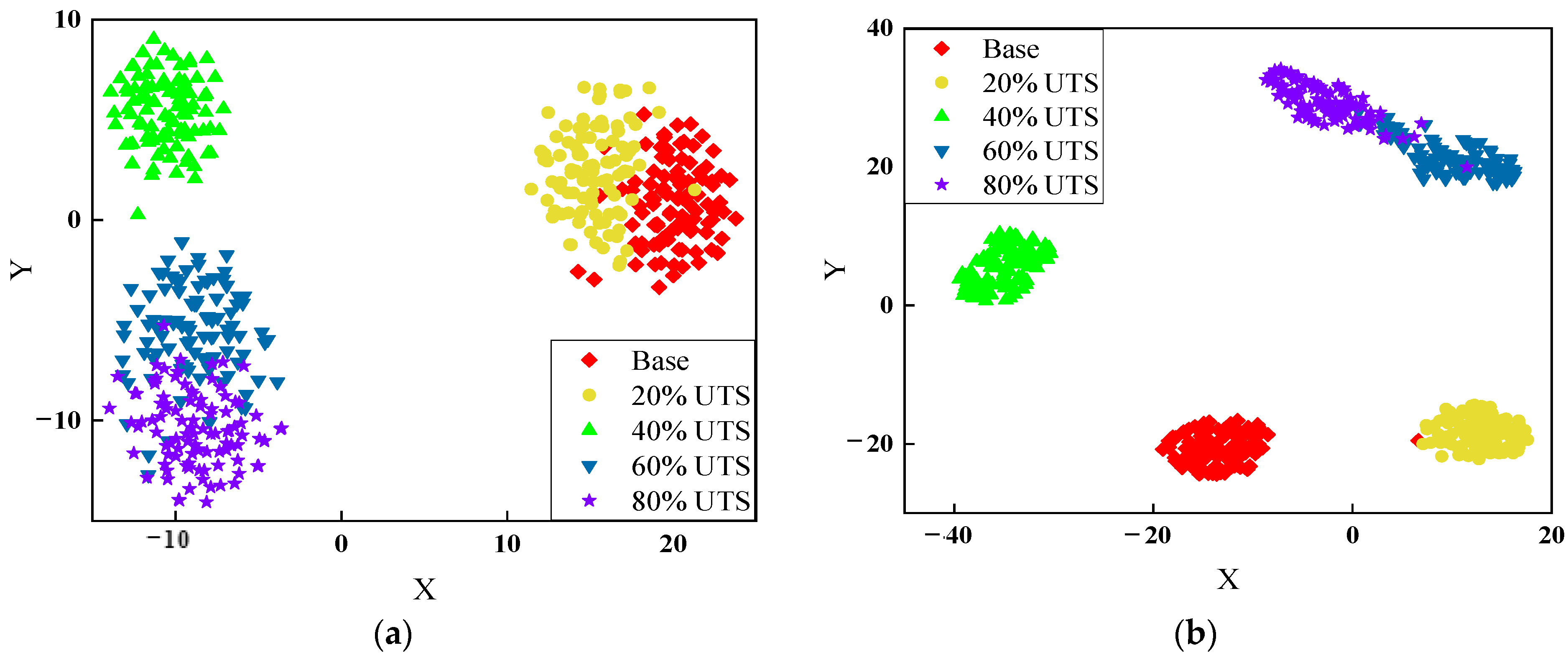
Figure 8 depicts the features in Case 1, where the prestress level of the unembedded rod is 80 dB. States #1–5 represent the rod with the prestress level equal to 0% (base state), 20% UTS, 40% UTS, 60% UTS, and 80% UTS. In total, 2500 samples comprised the dataset, where 1500 were used to train the model, 500 for validation, and the remaining 500 for testing. Figure 8a displays the feature maps of the test set after the first convolutional layer. Through the distribution of features, data labeled as 40% UTS (green upper triangle) were isolated from the entire dataset. This indicates that the features in this label extracted from the first layer of the CNN model were much easier to separate than others because the Euclidean distance is larger. However, the clusters in the red diamond (base state) and yellow circle (20% UTS) located on the right side overlapped. At least one-quarter of the data were mixed and difficult to separate, which means errors will occur. In addition, the rod samples prestressed in 60% UTS (blue lower triangle) and 80% UTS (purple star) were tangled together. Figure 8b represents the feature maps from the last layer of the CNN. After eight layers’ processing, most of the samples were separated, except one outlier in the base class clustered in 20% UTS and a small overlap appeared between the samples in 60% UTS and 80% UTS. The results demonstrate that the features became more sensitive after operating the whole CNN process.
The CNN model sliced input signals into several small pieces, which enlarged the sensitive features and cut off the excess. Figure 9 plots the feature maps from five different prestress levels after three convolutional layers. The data are signals from five different prestress levels in Case 1 when SNR is equal to 100 dB. The differences between the five figures are clear. The shape and peak values of lines characterize signals from different groups. However, with the increasing noise level, extracting features became harder.
Figure 10 illustrates the feature visualization in Case 1 when SNRs were equal to 100 dB, 70 dB, and 60 dB. At 100 dB (in Figure 10a), the five clusters were far from each other, and each cluster of data is relatively concentrated, with an average standard deviation close to 2.53. With the noise level increased to 80 dB (shown in Figure 10b), a small overlap appeared between the 60% UTS and 80% UTS data, but the other three groups were clearly separated. The standard deviation in this situation was large, 2.83. However, when SNR was lower than 80 dB, the distributions of features changed dramatically. At 70 dB, features in either the base state and 20% UTS or 60% UTS and 80% UTS were blended into each other, and only the data in the green upper triangles were independently located below the graph, demonstrated in Figure 10b. In Figure 10c, feature maps at 60 dB had a worse situation, as all the data interwove together entirely. It is hard to ascertain the boundaries of each group. Therefore, this proved that noise had an adverse effect on the feature extraction of the CNN.

4.2. Classification for Prestress Levels of the Rod by CNN

The performance of CNN trained by the data under various noise levels is shown in Figure 11, which classified the prestress levels of the rod in Case 1. Of the 2500 data points, 1500 were used for training the CNN model, and the training curves are illustrated in Figure 11a. Specifically, these training curves started near 20%, and then converged to 100%. When the noise level was 100 dB, the model only spent seven epochs to improve the accuracy to 100%. That epoch number was enlarged to 25 at 90 dB. With SNR increased, more epochs were spent on converging, and the error reduced to 0 with 34 epochs at 80 dB. The slope of training curves from 100 dB to 80 dB were much larger than the curves at 70 dB and 60 dB. In detail, the accuracy of classification was raised from 20% to 31% by 15 epochs at 60 dB and then close to 100% after the 30th epoch. The validation set included 500 data points for modifying the parameters in CNN. The validation curves for 40 epochs showed that the accuracy of CNN started at 20% and increased with the epochs. At 100 dB and 90 dB, the accuracies reached 100% after training 6 and 20 epochs, respectively. When SNR was 80 dB, the curve was close to 0.98 after the 28th epoch and would not improve as the epoch increased. However, the accuracies were lower at 70 dB and 60 dB, where the curve converged to 0.78 and 0.34 after training 40 epochs. Approximately 32% of the data were misjudged as the incorrect category at 70 dB. The situation at 60 dB was much worse, as most of the data could not be classified into the right category.
The test results at various noise levels are shown in Table 3. When SNR was no less than 90 dB, the CNN model classified the test data correctly into the corresponding categories because the training curves and the validation curves reached 100% after training. At 80 dB, the accuracy of test data was 98%, and some misjudgments appeared in the base state and the 80% UTS state. The results of the feature map visualization show that some data in the base state were dropped into the 20% UTS group, and the 60% UTS and 80% UTS clusters overlapped (shown in Figure 11b). The mixed features caused the misjudgments in the test. At 70 dB, only 74% of the data were identified correctly, and 25% of the data in the first category were misclassified into the second category. On the contrary, 27% of the data that belonged to the second category were placed into the first category. The accuracies of the fourth and fifth categories were both equal to 63%. The conclusion is consistent with the previous analysis in feature visualization and accurate curves. At 60 dB, the CNN model was not suitable in this situation because the noise covered the signals entirely and all the analysis focused on the noise. Thus, all results had low accuracy.
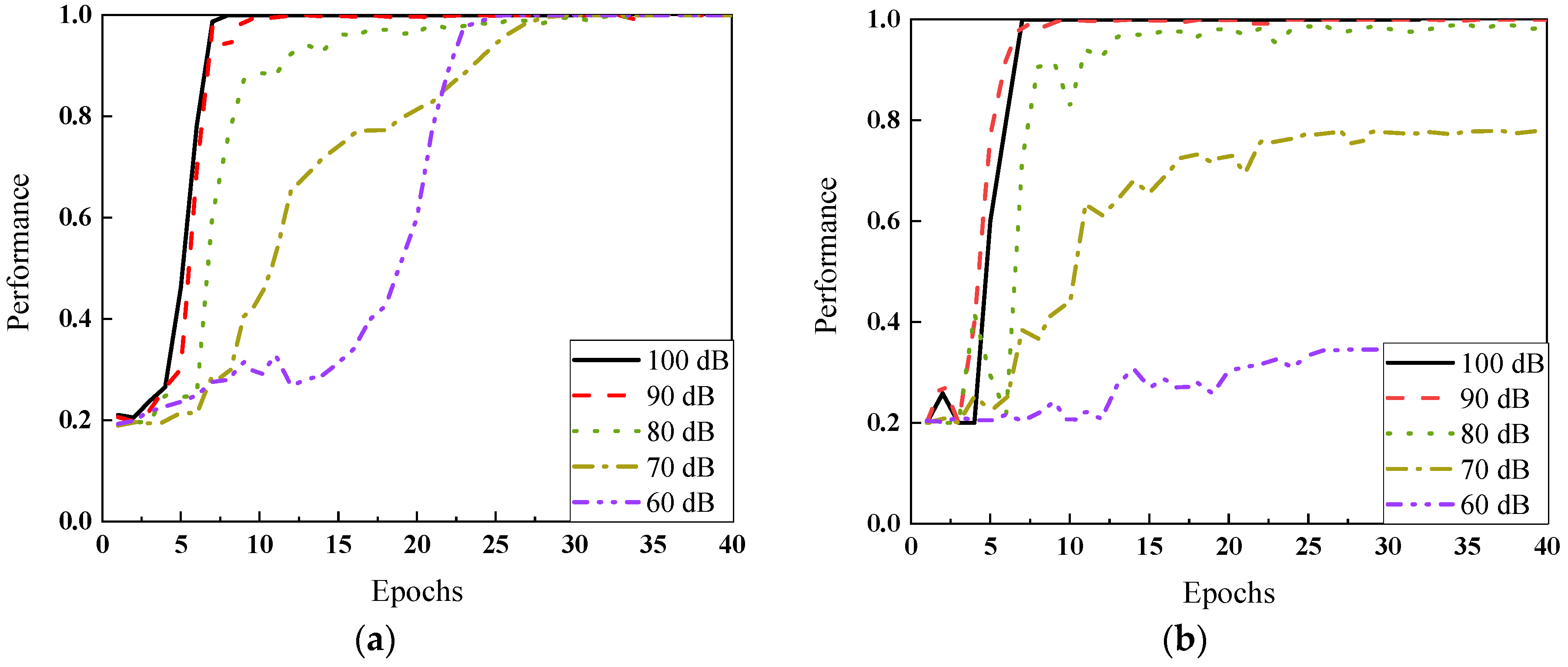
The performance of the CNN classifier in Cases 2 and 3 is shown in Figure 12. In Case 2, rods were embedded in cement. The training and validation results at five noise levels are illustrated in Figure 12a. The training and validation curves had better results when SNRs were higher than 70 dB. All the curves fluctuated during the first five epochs and then quickly converged to 0. Nearly 10 epochs were spent to increase the accuracies to 100%. At 70 dB, although the training curve took about 20 epochs to converge to 100%, the validation curve only reached 0.78. However, the performance of the CNN dropped sharply at 60 dB. In Case 3, the error occurred at 80 dB, where the training accuracy and validation accuracy were close to 0.99 and 0.94, respectively. The error rate increased at 70 dB, where the validation curve reached 0.77 at the 20th epoch and then flattened out. The results in Case 3 were similar to those of Case 1 because the grease had less of an effect on guided wave propagation.
The test results of Cases 2 and 3 are shown in Table 4 when SNRs were from 90 dB to 60 dB. In Case 2, all the test data were identified correctly at 90 dB and 80 dB. At 70 dB, only the base state had a classification rate of 98%, and the other four groups had lower rates. Among them, 12 of 100 data samples in the second category were misclassified into the third and fourth categories. The accuracy of the third category was 74% with 26% misjudgment. In addition, the error rates in the fourth and fifth categories were 66% and 64%, respectively. When the noise level increased to 60 dB, the accuracy of prestress identification was the lowest (46.6%). Most of the data could not be identified, except the data in the base condition (at 99%). Compared with Case 2, the approach exhibited a slightly lower accuracy for Case 3, where 100% of data in 90 dB were classified, 94.4% were identified at 80 dB, 76% at 70 dB, and 41.6% at 60 dB. At 80 dB and 70 dB, most of the errors occurred between the fourth and fifth categories. Specifically, the predictions of the fourth and fifth categories reached 78% and 94% at 80 dB. At 70 dB, the proportions were reduced to 52% and 51%, respectively. At 60 dB, only the data under the base condition could be identified, and it was hard to identify the data in other conditions.

4.3. Classification for Embedding Situation by CNN

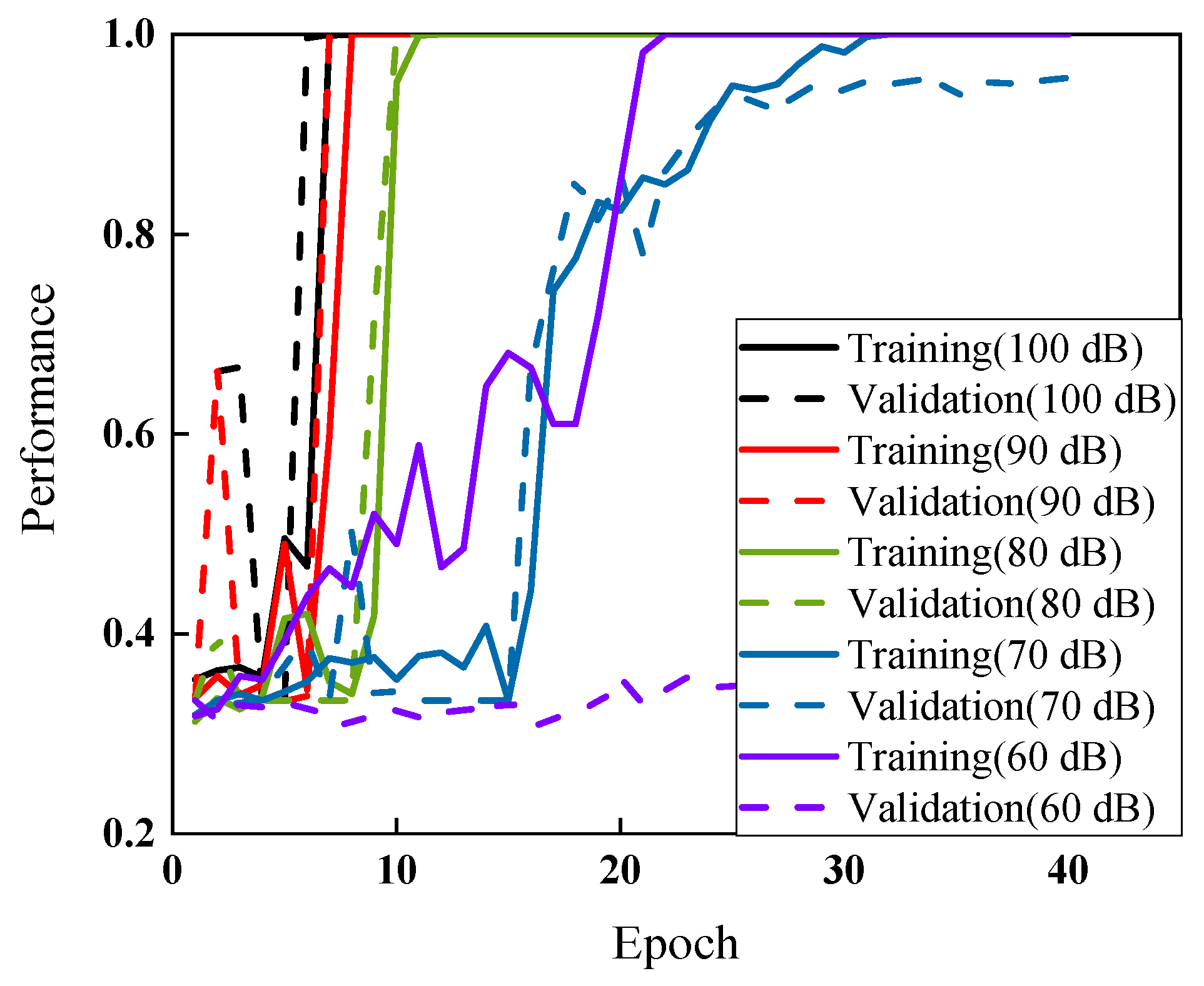
The embedding situation of the rod could also be predicted by the CNN classifier. A total of 1500 data points were used for training the CNN, including unembedded rods, rods embedded with cement, and rods embedded with grease. The training and validation curves are shown in Figure 13. At a lower noise level, the classifier entirely predicted the state of the rod. Until SNR was 70 dB, the validation curve was 0.956, training 40 epochs. However, the accuracies at 60 dB dropped sharply. The test results are given in Table 5. Predictions were equal to 100% in each category when SNRs were from 100 dB to 80 dB. Several errors occurred at 70 dB and the accuracy was 92%. Specifically, the rod samples labeled as unembedded were much easier to confuse as rods embedded in grease, as 15% of the data in that category were misclassified into the grease state. On the other hand, 7% of the data were misclassified into the unembedded state. Only 1% of data in cement were predicted incorrectly. The worst results were the classification at 60 dB, where the total accuracy was only 35%, which means the model cannot identify the signals.

5. Conclusions

We investigated the deep learning-based guided wave process for stress level prediction of prestressed rods. The CNN model was established for automatically encoding the hidden information from complex signals that accounted for the impacts of different noise levels and embedded grout materials. Some conclusions can be listed as follows:
(a)
The deep learning method effectively encoded the guided waves under complex uncertainties and assisted in stress level prediction and the embedded conditions of the rods, thereby showing potential for signal processing of NDE methods in structural health monitoring of PC structures.
(b)
The feature visualization method, t-SNE, provided an effective window that the different feature patterns could be clearly identified from visual two-dimensional plots. The distances between each feature point indicated the correlation among data. In addition, the impacts of noise interference on the data were observed with the use of this approach.
(c)
The deep learning approach also exhibited high accuracy and robustness for data with high noise interference. The CNN classification for most cases could reach up to 100% when the noise levels were lower (80 dB–100 dB). However, with the energy of the noise (SNR = 70 dB) close to the signals, data classification exhibited a certain level of reduction, and the error rates were close to 80%. Particularly, when the noise increased to a much higher level (60 dB), all the signals were contaminated, and the effectiveness of the classification dropped.
(d)
The proposed method can also identify the embedding conditions. The identification is no less than 92% when the noise level is lower than 60 dB. However, the accuracy drops to 35% at 60 dB, which means it is difficult to distinguish the embedding conditions of rods.
This study simulated the different levels of PC structure’s prestress loss by a deep learning method. To accommodate engineering concerns, noise interference was added. In future work, the methods will be explored on more large-scale structures in laboratory and field conditions. As high levels of noise prevent the model from achieving high accuracy, future perspective will focus on this issue to improve the accuracy of identification under higher noise levels (60 dB). In addition, different kinds of damage will occur at same time; thus, future study will investigate more complex situations. Furthermore, as the selection of hyperparameters is also critical, future research will also focus on deep learning with optimization methods (Bayesian optimization).

Author Contributions

Z.Z. designed, conducted research, and wrote the paper under the supervision of Z.L.; F.T. and Q.C. edited the paper; H.P. and X.W. assisted with the experiments and edited the paper. All authors have read and agreed to the published version of the manuscript.

Funding

This research received no external funding.

Conflicts of Interest

The authors declare no conflict of interest.

References

  1. Gui, G.; Pan, H.; Lin, Z.; Li, Y.; Yuan, Z. Data-driven support vector machine with optimization techniques for structural health monitoring and damage detection. KSCE J. Civ. Eng. 2017, 21, 523–534. [Google Scholar] [CrossRef]
  2. Tang, F.; Lin, Z.; Chen, G.; Yi, W. Three-dimensional corrosion pit measurement and statistical mechanical degradation analysis of deformed steel bars subjected to accelerated corrosion. Constr. Build. Mater. 2014, 70, 104–117. [Google Scholar] [CrossRef]
  3. Lin, Z.; Mostafa, F.; Wu, C.H.; Chen, G.; Bevans, W.J.; Gunasekaran, A.V.K.; Sedigh, S. Design, Construction, Laboratory and Field Testing of the Bridge on the Arnault Branch, Washington County, Missouri. In Center for Transportation Infrastructure and Safety/NUTC Program; Missouri University of Science and Technolog: Rolla, MO, USA, 2013. [Google Scholar]
  4. Bartoli, I.; Salamone, S.; Phillips, R.; Lanza di Scalea, F.; Sikorsky, C.S. Use of Interwire Ultrasonic Leakage to Quantify Loss of Prestress in Multiwire Tendons. J. Eng. Mech. 2011, 137, 324–333. [Google Scholar] [CrossRef]
  5. Chen, S.Z.; Wu, G.; Feng, D.C.J.M.S.; Processing, S. Damage detection of highway bridges based on long-gauge strain response under stochastic traffic flow. Mech. Syst. Signal Process. 2019, 127, 551–572. [Google Scholar] [CrossRef]
  6. Zhang, Z.; Pan, H.; Wang, X.; Tang, F.; Lin, Z. Ultrasonic guided wave approaches for pipeline damage diagnosis based on deep leaning. In Proceedings of the ASCE Pipelines 2022 Conference, Indianapolis, IN, USA, 31 July–3 August 2022. [Google Scholar]
  7. Zhang, Z.; Pan, H.; Wang, X.; Lin, Z. Machine learning-enabled Lamb wave approaches for damage detection. In Proceedings of the 2021 10th International Conference on Structural Health Monitoring of Intelligent Infrastructure, Porto, Portugal, 30 June–2 July 2021. [Google Scholar]
  8. Tang, F.; Lin, Z.; Qu, H. Investigation into corrosion-induced bond degradation between concrete and steel rebar with acoustic emission and 3D laser scan techniques. J. Infrastruct. Preserv. Resil. 2022, 3, 1–18. [Google Scholar] [CrossRef]
  9. Zhang, Y.M.; Wang, H.; Bai, Y.; Mao, J.X.; Xu, Y.C. Bayesian dynamic regression for reconstructing missing data in structural health monitoring. Struct. Health Monit. 2022, 21, 2097–2115. [Google Scholar] [CrossRef]
  10. Beard, M.; Lowe, M.; Cawley, P. Ultrasonic guided waves for inspection of grouted tendons and bolts. J. Mater. Civ. Eng. 2003, 15, 212–218. [Google Scholar] [CrossRef]
  11. Cobb, A.C.; Kwun, H.; Caseres, L.; Janega, G. Torsional guided wave attenuation in piping from coating, temperature, and large-area corrosion. NDT E Int. 2012, 47, 163–170. [Google Scholar] [CrossRef]
  12. Zhang, Z.; Pan, H.; Wang, X.; Lin, Z. Machine Learning-Enriched Lamb Wave Approaches for Automated Damage Detection. Sensors 2020, 20, 1790. [Google Scholar] [CrossRef] [Green Version]
  13. Zhang, Z.; Pan, H.; Wang, X.; Lin, Z. Deep Learning Empowered Structural Health Monitoring and Damage Diagnostics for Structures with Weldment via Decoding Ultrasonic Guided Wave. Sensors 2022, 22, 5390. [Google Scholar] [CrossRef]
  14. Sun, H.; Zhu, J. Nondestructive evaluation of steel-concrete composite structure using high-frequency ultrasonic guided wave. Ultrasonics 2020, 103, 106096. [Google Scholar] [CrossRef]
  15. Lanza di Scalea, F.; Rizzo, P.; Seible, F. Stress measurement and defect detection in steel strands by guided stress waves. J. Mater. Civ. Eng. 2003, 15, 219–227. [Google Scholar] [CrossRef]
  16. Ervin, B.L.; Kuchma, D.A.; Bernhard, J.T.; Reis, H. Monitoring corrosion of rebar embedded in mortar using high-frequency guided ultrasonic waves. J. Eng. Mech. 2009, 135, 9–19. [Google Scholar] [CrossRef]
  17. Chaki, S.; Bourse, G. Guided ultrasonic waves for non-destructive monitoring of the stress levels in prestressed steel strands. Ultrasonics 2009, 49, 162–171. [Google Scholar] [CrossRef]
  18. Treyssede, F.; Laguerre, L. Investigation of elastic modes propagating in multi-wire helical waveguides. J. Sound Vib. 2010, 329, 1702–1716. [Google Scholar] [CrossRef] [Green Version]
  19. Dubuc, B.; Ebrahimkhanlou, A.; Salamone, S. Higher order longitudinal guided wave modes in axially stressed seven-wire strands. Ultrasonics 2018, 84, 382–391. [Google Scholar] [CrossRef]
  20. Shoji, M. Ultrasonic Guided Wave Inspection of Anchor Rods Embedded in Soil. J. Nondestruct. Eval. 2019, 38, 96. [Google Scholar] [CrossRef]
  21. Pan, H.; Gui, G.; Lin, Z.; Yan, C. Deep BBN learning for health assessment toward decision-making on structures under uncertainties. KSCE J. Civ. Eng. 2018, 22, 928–940. [Google Scholar] [CrossRef]
  22. Lin, Z.; Pan, H.; Wang, X.; Li, M. Data-driven structural diagnosis and conditional assessment: From shallow to deep learning. In Proceedings of the Sensors and Smart Structures Technologies for Civil, Mechanical, and Aerospace Systems 2018, Denver, CO, USA, 4–8 March 2018; International Society for Optics and Photonics: Bellingham, WA, USA, 2018; p. 1059814. [Google Scholar]
  23. Abdeljaber, O.; Avci, O.; Kiranyaz, S.; Gabbouj, M.; Inman, D.J. Real-time vibration-based structural damage detection using one-dimensional convolutional neural networks. J. Sound Vib. 2017, 388, 154–170. [Google Scholar] [CrossRef]
  24. Fawaz, H.I.; Forestier, G.; Weber, J.; Idoumghar, L.; Muller, P.-A. Deep learning for time series classification: A review. Data Min. Knowl. Discov. 2019, 33, 917–963. [Google Scholar] [CrossRef]
  25. Pan, H.; Azimi, M.; Yan, F.; Lin, Z. Time-frequency-based data-driven structural diagnosis and damage detection for cable-stayed bridges. J. Bridge Eng. 2018, 23, 04018033. [Google Scholar] [CrossRef]
  26. Zhang, Z.; Wang, X.; Pan, H.; Lin, Z. Corrosion-induced damage identification in metallic structures using machine learning approaches. In Proceedings of the 2019 Defense TechConnect Innovation Summit, National Harbor, MD, USA, 7–10 October 2019. [Google Scholar]
  27. Cha, Y.J.; Choi, W.; Büyüköztürk, O. Deep learning-based crack damage detection using convolutional neural networks. Comput. Aided Civ. Infrastruct. Eng. 2017, 32, 361–378. [Google Scholar] [CrossRef]
  28. Cha, Y.J.; Choi, W.; Suh, G.; Mahmoudkhani, S.; Büyüköztürk, O. Autonomous structural visual inspection using region-based deep learning for detecting multiple damage types. Comput. Aided Civ. Infrastruct. Eng. 2018, 33, 731–747. [Google Scholar] [CrossRef]
  29. An, Y.-K.; Jang, K.; Kim, B.; Cho, S. Deep learning-based concrete crack detection using hybrid images. In Proceedings of the Sensors and Smart Structures Technologies for Civil, Mechanical, and Aerospace Systems 2018, Denver, CO, USA, 4–8 March 2018; International Society for Optics and Photonics: Bellingham, WA, USA, 2018; p. 1059812. [Google Scholar]
  30. Pan, H.; Zhang, Z.; Wang, X.; Lin, Z. Image-based damage conditional assessment of large-scale infrastructure systems using remote sensing and deep learning approaches. In Proceedings of the 2019 TechConnect World Innovation Conference, Boston, MA, USA, 17–19 June 2019. [Google Scholar]
  31. Guo, J.; Xie, X.; Bie, R.; Sun, L. Structural health monitoring by using a sparse coding-based deep learning algorithm with wireless sensor networks. Pers. Ubiquitous Comput. 2014, 18, 1977–1987. [Google Scholar] [CrossRef]
  32. Zhang, W.; Peng, G.; Li, C.; Chen, Y.; Zhang, Z. A new deep learning model for fault diagnosis with good anti-noise and domain adaptation ability on raw vibration signals. Sensors 2017, 17, 425. [Google Scholar] [CrossRef] [Green Version]
  33. Mahajan, H.; Banerjee, S. A machine learning framework for guided wave-based damage detection of rail head using surface-bonded piezo-electric wafer transducers. Mach. Learn. Appl. 2021, 7, 100216. [Google Scholar] [CrossRef]
  34. Tabian, I.; Fu, H.; Sharif Khodaei, Z. A Convolutional Neural Network for Impact Detection and Characterization of Complex Composite Structures. Sensors 2019, 19, 4933. [Google Scholar] [CrossRef] [Green Version]
  35. Zargar, S.A.; Yuan, F.-G. Impact diagnosis in stiffened structural panels using a deep learning approach. Struct. Health Monit. 2021, 20, 681–691. [Google Scholar] [CrossRef]
  36. Chree, C. The equations of an isotropic elastic solid in polar and cylindrical co-ordinates their solution and application. TCaPS 1889, 14, 250. [Google Scholar]
  37. Raghavan, A.; Cesnik, C.E. 3-D elasticity-based modeling of anisotropic piezocomposite transducers for guided wave structural health monitoring. J. Vib. Acoust. 2007, 129, 739–751. [Google Scholar] [CrossRef]
  38. Seco, F.; Martín, J.M.; Jiménez, A.; Pons, J.L.; Calderón, L.; Ceres, R. PCDISP: A tool for the simulation of wave propagation in cylindrical waveguides. In Proceedings of the 9th International Congress on Sound and Vibration, Orlando, FL, USA, 8–11 July 2002. [Google Scholar]
  39. Seco, F.; Jiménez, A.R. Modelling the generation and propagation of ultrasonic signals in cylindrical waveguides. Ultrason. Waves 2012, 1–28. [Google Scholar] [CrossRef]
  40. Beard, M.; Lowe, M. Non-destructive testing of rock bolts using guided ultrasonic waves. Int. J. Rock Mech. Min. Sci. 2003, 40, 527–536. [Google Scholar] [CrossRef]
  41. Haskins, R.W. Detection of Microcracks in Trunnion Rods Using Ultrasonic Guided Waves. 2015. Available online: https://apps.dtic.mil/sti/pdfs/ADA619008.pdf (accessed on 23 September 2022).
  42. Zhang, B.; Hong, X.; Liu, Y. Multi-task deep transfer learning method for guided wave-based integrated health monitoring using piezoelectric transducers. IEEE Sens. J. 2020, 20, 14391–14400. [Google Scholar] [CrossRef]
  43. Liang, X. Image-based post-disaster inspection of reinforced concrete bridge systems using deep learning with Bayesian optimization. Comput. Aided Civ. Infrastruct. Eng. 2019, 34, 415–430. [Google Scholar] [CrossRef]
  44. Zhang, Y.-M.; Wang, H.; Mao, J.-X.; Xu, Z.-D.; Zhang, Y.-F. Probabilistic framework with bayesian optimization for predicting typhoon-induced dynamic responses of a long-span bridge. J. Struct. Eng. 2021, 147, 04020297. [Google Scholar] [CrossRef]
  45. Gulgec, N.S.; Takáč, M.; Pakzad, S.N. Structural damage detection using convolutional neural networks. In Model Validation and Uncertainty Quantification, Volume 3; Springer: Cham, Switzerland, 2017; pp. 331–337. [Google Scholar]
  46. Maaten, L.v.d.; Hinton, G. Visualizing data using t-SNE. J. Mach. Learn. Res. 2008, 9, 2579–2605. [Google Scholar]
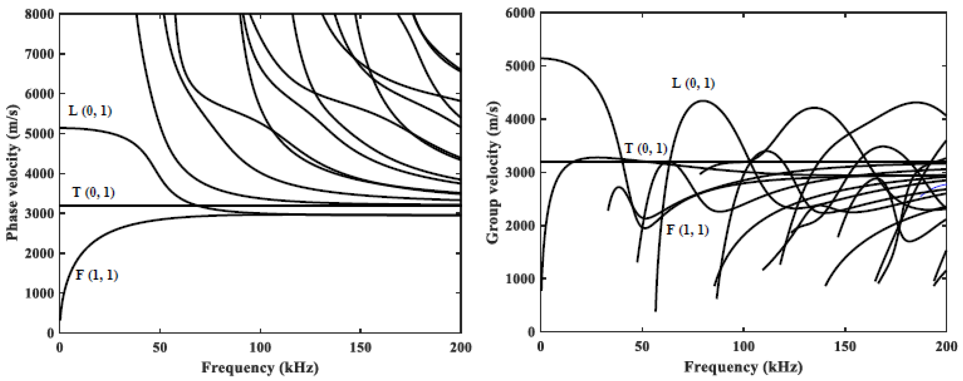
Figure 1. Phase velocities and group velocities.
Buildings 12 01772 g001
Figure 2. Calibration of the FE model. (a) Meshing of the rod embedded in concrete. (b) Comparison of signals with the literature.
Buildings 12 01772 g002
Figure 3. Rod models.
Buildings 12 01772 g003
Figure 4. Received signals at different stress levels: (a) zero; (b) 20% UST; (c) 40% UTS; (d) 60% UTS; (e) 80% UTS.
Buildings 12 01772 g004
Figure 5. Received signals for rods with different grout methods: (a) no grout; (b) grease; (c) cement.
Buildings 12 01772 g005
Figure 6. Received signals at different noise levels.
Buildings 12 01772 g006
Figure 7. Flowchart of CNN.
Buildings 12 01772 g007
Figure 8. Feature visualization by t-SNE. (a) Feature maps in the first convolutional layer; (b) feature maps in the last layer.
Buildings 12 01772 g008
Figure 9. Feature maps: (a) 0% UTS; (b) 20% UTS; (c) 40% UTS; (d) 60% UTS; (e) 80% UTS.
Buildings 12 01772 g009
Figure 10. Feature visualization by t-SNE. (a) SNR = 100 dB; (b) SNR = 70 dB; (c) SNR = 60 dB.
Buildings 12 01772 g010
Figure 11. Learning results of CNN at various noise levels. (a) Training curve; (b) test curve.
Buildings 12 01772 g011
Figure 12. Results of CNN at various noise levels. (a) Case 2; (b) Case 3.
Buildings 12 01772 g012
Figure 13. Results of CNN at various noise levels.
Buildings 12 01772 g013
Table 1. Test matrix for computation modeling.
CaseStatePrestressing Level
(UTS)
Grout MaterialNoise Level
1
(no grout)
# 1zero\100 dB–60 dB
# 220%\
# 340%\
# 460%\
# 580%\
2
(grease)
# 6zeroGrease
# 720%Grease
# 840%Grease
# 960%Grease
# 1080%Grease
3
(cement)
# 11zeroCement
# 1220%Cement
# 1340%Cement
# 1460%Cement
# 1580%Cement
Table 2. Details of the proposed CNN.
NameFiltersFilter SizeStrideBiasOutput Layer Size
Input layer--------1000 × 4
Convolutional layer (C1)2025 × 2120976 × 3
Max pooling layer (P1)205 × 15--195 × 3
Convolutional layer (C2)4025 × 3140171 × 1
Max pooling layer (P1)405 × 15--34 × 1
Convolutional layer (C3)205 × 112030 × 1
ReLU--------30 × 1
Fully connected layer (F1)530 × 1155
Softmax--------5
Table 3. Confusion matrices at various noise levels.
90 dB (100%)80 dB (98%)
Base20%40%60%80%Base20%40%60%80%
Base100.0%0.0%0.0%0.0%0.0%99.0%0.0%0.0%0.0%0.0%
20%0.0%100.0%0.0%0.0%0.0%1.0%100%0.0%0.0%0.0%
40%0.0%0.0%100.0%0.0%0.0%0.0%0.0%100%0.0%0.0%
60%0.0%0.0%0.0%100.0%0.0%0.0%0.0%0.0%98%7.0%
80%0.0%0.0%0.0%0.0%100.0%0.0%0.0%0.0%2.0%93.0%
70 dB (74%)60 dB (26.8%)
Base75%27.0%0.0%0.0%0.0%28.0%27.0%20.0%12.0%15.0%
20%25.0%71.0%1.0%0.0%0.0%28.0%22.0%17.0%15.0%12.0%
40%0.0%0.0%98%0.0%0.0%20.0%16.0%34.0%17.0%22.0%
60%0.0%1.0%1.0%63.0%37.0%14.0%14.0%12.0%23.0%15.0%
80%0.0%1.0%0.0%37.0%63.0%10.0%21.0%17.0%33.0%36.0%
Table 4. Confusion matrices in Case 2 and 3.
Case 2 (Grease as the Grout Material)
90 dB (100%)80 dB (100%)
Base20%40%60%80%Base20%40%60%80%
Base100.0%0.0%0.0%0.0%0.0%100.0%0.0%0.0%0.0%0.0%
20%0.0%100.0%0.0%0.0%0.0%0.0%100.0%2.0%5.0%4.0%
40%0.0%0.0%100.0%0.0%0.0%0.0%8.0%100.0%15.0%18.0%
60%0.0%0.0%0.0%100.0%0.0%0.0%4.0%14.0%100.0%14.0%
80%0.0%0.0%0.0%0.0%100.0%0.0%0.0%10.0%14.0%100.0%
70 dB (78%)60 dB (46.6%)
Base98%0.0%0.0%0.0%0.0%99%1%0%1%0%
20%2.0%88%2.0%5.0%4.0%0%50%16%29%8%
40%0.0%8.0%74%15.0%18.0%0%13%24%16%25%
60%0.0%4.0%14.0%66%14.0%1%26%31%26%33%
80%0.0%0.0%10.0%14.0%64.0%0%10%29%28%34%
Case 3 (Cement as the grout material)
90 dB (100%)80 dB (94.4%)
Base100.0%0.0%0.0%0.0%0.0%100.0%0.0%0.0%0.0%0.0%
20%0.0%100.0%0.0%0.0%0.0%0.0%100.0%0.0%0.0%0.0%
40%0.0%0.0%100.0%0.0%0.0%0.0%0.0%100.0%0.0%0.0%
60%0.0%0.0%0.0%100.0%0.0%0.0%0.0%0.0%78.0%6.0%
80%0.0%0.0%0.0%0.0%100.0%0.0%0.0%0.0%22.0%94.0%
70 dB (76%)60 dB (41.6%)
Base99.0%1.0%0.0%0.0%0.0%79.0%18.0%2.0%5.0%3.0%
20%0.0%99.0%0.0%0.0%0.0%18.0%38.0%20.0%9.0%11.0%
40%1.0%0.0%79.0%13.0%12.0%1.0%19.0%29.0%29.0%23.0%
60%0.0%0.0%11.0%52.0%37.0%1.0%15.0%25.0%27.0%28.0%
80%0.0%0.0%10.0%35.0%51.0%1.0%10.0%24.0%30.0%35.0%
Table 5. Confusion matrices in varying embedding conditions.
90 dB (100%)80 dB (100%)
UnembeddedCementGreaseUnembeddedCementGrease
Unembedded100.0%0.0%0.0%100.0%0.0%0.0%
Cement0.0%100.0%0.0%0.0%100.0%0.0%
Grease0.0%0.0%100.0%0.0%0.0%100.0%
70 dB (92%)60 dB (35%)
Unembedded84.0%0.0%7.0%37.0%24.0%39.0%
Cement1.0%99.0%0.0%28.0%43.0%36.0%
Grease15.0%1.0%93.0%35.0%33.0%25.0%
Publisher’s Note: MDPI stays neutral with regard to jurisdictional claims in published maps and institutional affiliations.