Study Using Machine Learning Approach for Novel Prediction Model of Liquid Limit

Abstract

The liquid limit (LL) is considered the most fundamental parameter in soil mechanics for the design and analysis of geotechnical systems. According to the literature, the LL is governed by different particle sizes such as sand content (S), clay content (C), and silt content (M). However, conventional methods do not incorporate the effect of all the influencing factors because traditional methods utilize material passing through a # 40 sieve for LL determination (LL₄₀), which may contain a substantial number of coarse particles. Therefore, recent advancements suggest that the LL must be determined using material passing from a # 200 sieve. However, determining the liquid limit using # 200 sieve material, referred to as LL₂₀₀ in the laboratory, is a time-consuming and difficult task. In this regard, artificial-intelligence-based techniques are considered the most reliable and robust solutions to such issues. Previous studies have adopted experimental routes to determine LL₂₀₀ and no such attempt has been made to propose empirical correlation for LL₂₀₀ determination based on influencing factors such as S, C, M, and LL₄₀. Therefore, this study presents a novel prediction model for the liquid limit based on soil particle sizes smaller than 0.075 mm (# 200 sieve) using gene expression programming (GEP). Laboratory experimental data were utilized to develop a prediction model. The results indicate that the proposed model satisfies all the acceptance requirements of artificial-intelligence-based prediction models in terms of statistical checks such as the correlation coefficient (R²), root-mean-square error (RMSE), mean absolute error (MAE), and relatively squared error (RSE) with minimal error. Sensitivity and parametric studies were also conducted to assess the importance of the individual parameters involved in developing the model. It was observed that LL₄₀ is the most significant parameter, followed by C, M, and S, with sensitivity values of 0.99, 0.93, 0.88, and 0.78, respectively. The model can be utilized in the field with more robustness and has practical applications due to its simple and deterministic nature.

1. Introduction

The liquid limit (LL) can be defined as the amount of water content at which soil behaves like a liquid and possesses the least possible measurable shear strength [1,2,3,4]. It is commonly employed for assessment of the physical and mechanical response of soils [5]. The most fundamental applications of the liquid limit are to classify fine-grained soils and determine its correlations with almost all the mechanical properties of cohesive soils such as the shear strength, compressive strength, consolidation behavior, stress history, shrink and swell characteristics, activity, toughness index, etc. [3,6].

The LL is commonly determined in the laboratory using the Casagrande method and fall cone method in accordance with ASTM standard 4318 [7] and BS 1377 [8]. The LL is used to classify fine-grained soils, which, according to the ASTM standard, are soils containing material having 50% or more particle sizes smaller than 0.075 mm [9]. However, it is conventionally determined based on # 40 sieve (0.425 mm particles) passing material [7]. The question is whether it is appropriate to determine the liquid limit using # 40 sieve passing material (LL₄₀), as it may contain coarse content referred to as medium fine-grained sand. This leads to major changes in soil classification and subsequent correlations of LL with the mechanical characteristics of soils. It has recently been established that the LL must be determined using # 200 sieve passing material (LL₂₀₀) instead of # 40 sieve passing material (LL₄₀), as the LL is governed by several particle sizes including sand content (S), silt content (M), and clay content (C) [10,11,12]. Therefore, this study is based on recent advancements in the context of determining the liquid limit based on # 200 sieve passing material. However, previous studies have adopted experimental routes to determine LL₂₀₀ and no such attempt, to the best of the authors’ knowledge, has been made to propose empirical correlation of LL₂₀₀ using artificial-intelligence-inspired techniques based on several influencing parameters.

However, determining LL₂₀₀ in a laboratory is a challenging task. In contrast to LL₄₀, which is conventionally calculated based on material that passes through a # 40 sieve, LL₂₀₀ requires extensive pulverization of dry soil particles in order for them to pass through a # 200 sieve’s opening widths (0.075 mm opening size). This makes it relatively difficult and time consuming to determine LL₂₀₀. Moreover, determination of influencing parameters such as clay content (C) and silt content (M) using hydrometer analysis requires cumbersome procedures. This constitutes the main motivation of the study: to propose a prediction model for LL₂₀₀ that not only saves time and provides high performance in terms of accuracy, but also incorporates critical influencing factors such as S, C, and M. Moreover, it is less likely that the liquid limit will be underestimated due to inaccuracy caused by LL₄₀. In this case, artificial intelligence (AI)-based prediction models are considered useful due to their capability to consider multiple influencing parameters, robustness, effectiveness in terms of cost and time, and capability to incorporate multiple influencing parameters [13,14,15,16].

It is worthwhile to note that the goal of the current study differs from the objectives of earlier studies because # 40 sieve material is the only type used in previous studies that consider the application of AI for determination of the LL. For instance, Seybold et al. [17] developed a prediction model for the estimation of Atterberg limits (PL and LL) based on clay content (C) and cation exchange capacity (CEC) as input variables, using a multiple linear regression technique (MLR). The study indicated that C and CEC play a vital role in determining Atterberg limits. Diaz et al. [18] proposed machine-learning-based models for determining Atterberg limits using the fall cone and Casagrande method. Similarly, Keller and Dexter [19] proposed relationships between Atterberg limits and clay content. However, these studies were based on liquid limit determination using # 40 sieve passing material and did not consider the liquid limit determination based on # 200 sieve passing material. Furthermore, it has been recognized well that LL depends on clay, silt, and coarse content [20]. Previous studies have adopted experimental routes for estimation of the LL using a # 200 sieve and no correlation exists, according to the authors’ best knowledge, to predict LL₂₀₀ using gene expression programming (GEP) and incorporating clay, silt, and sand content.

This research study aimed to propose a novel prediction model for LL₂₀₀ based on experimental data obtained from laboratory testing using gene expression programming. The soil samples were obtained from different locations in Pakistan and were tested in the laboratory to determine the liquid limit along with the basic index properties of soils such as sand (S), silt (M), and clay (C) contents. The proposed prediction model was validated through various statistical checks and error plots. Finally, sensitivity and parametric studies were also conducted to further justify the reliability of the proposed prediction model.

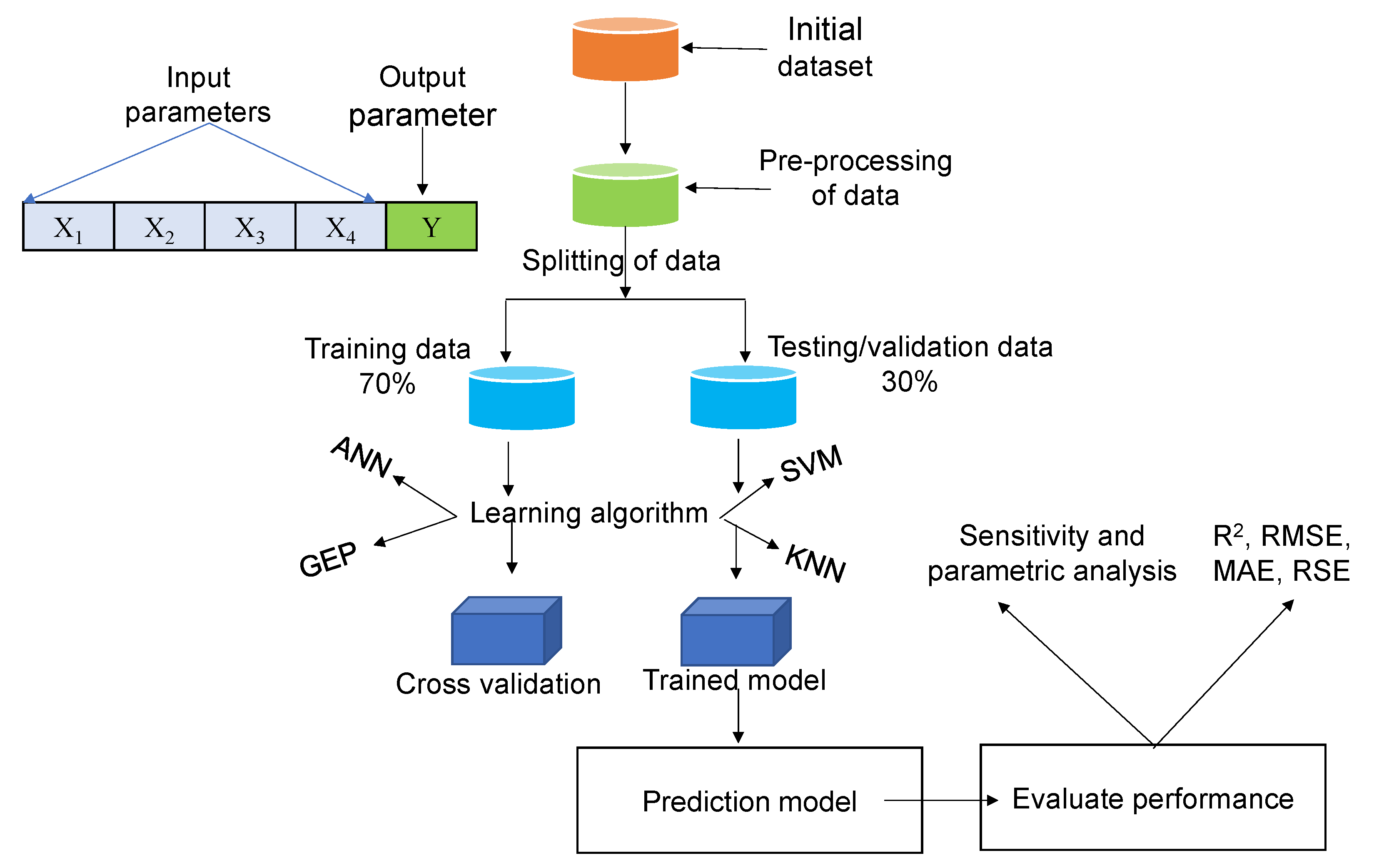
2. Research Methodology

The development of a prediction model using AI techniques requires authentic information supported by data either from laboratory or in-situ experimentation. The data are then processed by the selection of suitable input parameters in relation to the output variable. The data are further subdivided into training and validation categories. The use of AI techniques is a critical process and requires rigorous knowledge of computer vision. The model is trained, and performance is evaluated using different statistical checks. The general process involved in any prediction model development is illustrated in Figure 1.

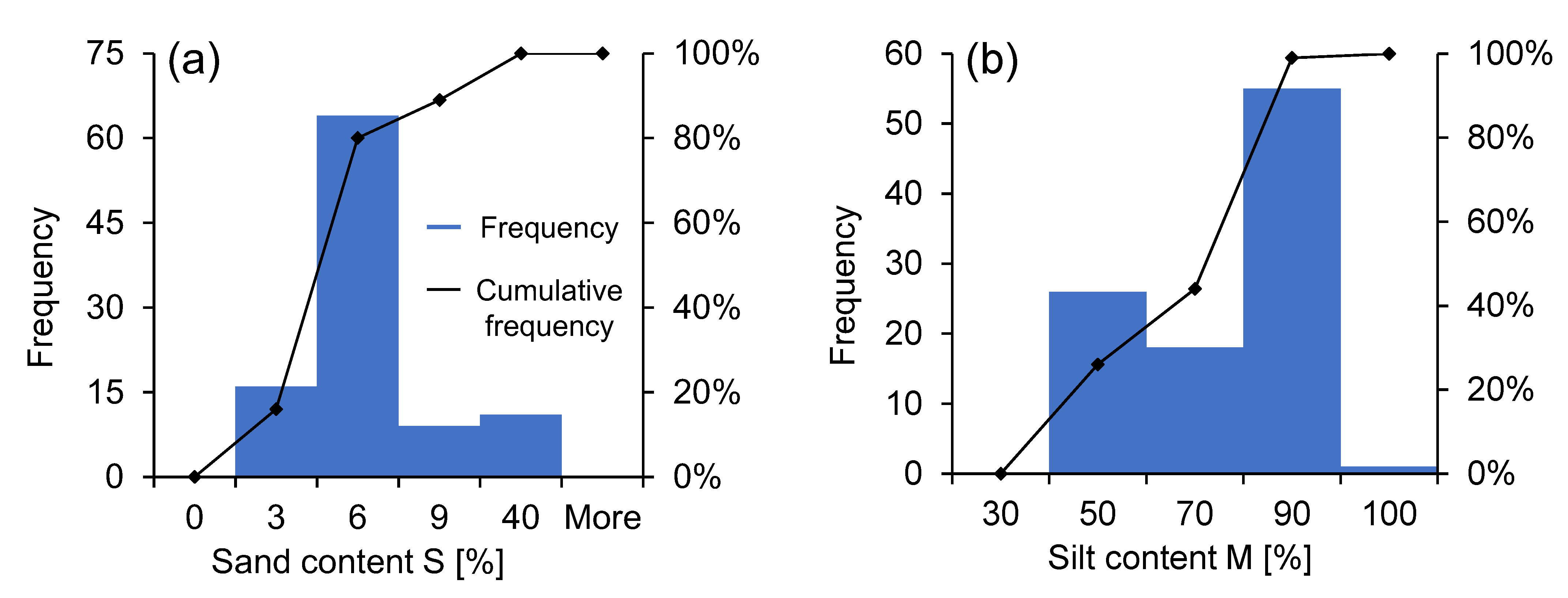
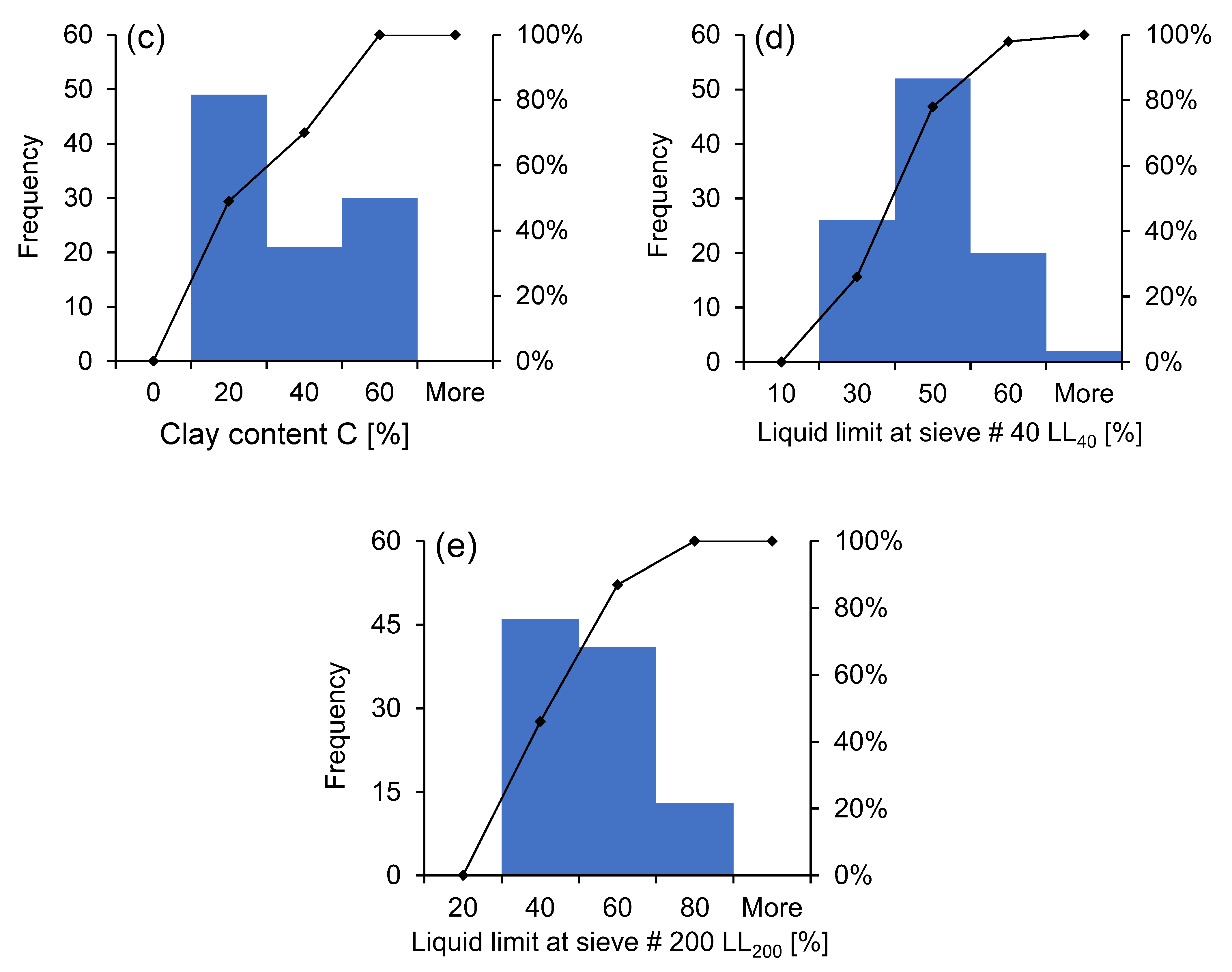
2.1. Data Collection

Soil samples were taken from different locations in Pakistan as shown in Figure 2 and were preserved for a laboratory testing program. The samples were collected from various regions using the hand auger method from shallow depths. Most of the regions are composed primarily of low plastic silty clay and sandy soils at shallow depths, followed by sandstones, gravelly clay, shale, and mudstone at greater depths. However, in this study, soil samples represent low plastic silty clay, which is also illustrated by laboratory results in the following sections.

2.2. Laboratory Testing and Results

In order to develop a prediction model, selection of critical and appropriate influencing input parameters is the fundamental process. It is well recognized from the literature that C, M, and S tend to influence the LL of cohesive soils [21]. Therefore, based on this rationale, S, M, C and LL₄₀ have been considered as the function of LL₂₀₀ as given by Equation (1).

$${\mathrm{LL}}_{200}=\mathrm{f}\left(\mathrm{S},\mathrm{C},\mathrm{M},{\mathrm{LL}}_{40}\right)$$

(1)

The laboratory testing program included the determination of basic index properties of soils such as sand content (S), clay content (C), silt content (M), liquid limit using # 40 (LL₄₀) and # 200 (LL₂₀₀) sieve passing materials.

Oven-dried soil samples were used to perform sieve analysis for the determination of sand and fine content in accordance with ASTM D 422 [22]. In this test, soils are passed through a succession of sieves ranging between # 4 (4.75 mm) and # 200 (0.075 mm) in descending order. The material retained in the # 200 sieve and passing from the # 4 sieve is termed as the sand content (S), whereas the material passing from the # 200 sieve is known as the fine content, which is further subdivided into C and M.

Since C (particle sizes smaller than 0.002 mm) and M (particle sizes between 0.075 and 0.002 mm) have very small sizes, they cannot be determined using sieve analysis. Therefore, hydrometer analysis inspired by Stokes’ law of particle sedimentation is used to determine C and M. In this test, soil particles having sizes smaller than 0.075 mm are mixed with water along with a dispersing agent (sodium hexameta phosphate or sodium silicate), and the relative movement of soil particles with regard to the hydrometer is recorded and interpreted to determine the size of particles in the suspension based on Stokes’ theorem of particle sedimentation. The percentage of particles having diameter ranges between 0.075 mm and 0.002 mm represents the silt content (M) whereas particle sizes smaller than 0.002 mm represent the clay content (C).

The LL can be determined using the Casagrande method and the fall cone method. In this study, the fall cone method was adopted due to its simplicity and time efficiency. A cone of apex angle 30° having a weight of 0.78 N is lowered into soil of varying moisture contents. The liquid limit is termed as the water content at which the penetration of the cone is 20 mm in five seconds of its free fall from a certain height. In this study, the liquid limit was determined using soils having particle sizes smaller than 0.075 mm and 0.425 mm separately and these are referred to as LL₄₀ and LL₂₀₀.

Figure 3 shows the histograms of frequency distribution of the data obtained from laboratory experiments. Figure 3a shows the frequency distribution of S determined from sieve analysis tests. The results indicate that S varies between 2% and 36%. Figure 3b indicates the frequency distribution of M, which varies between 34% and 93%. Figure 3c illustrates C varying between 5% and 60%. Similarly, Figure 3d,e show the frequency distribution of LL₄₀ and LL₂₀₀, which vary between 16% and 62%, and 23% and 70%, respectively. The results indicate that soil samples contain a diversity of soil types with a wide range of LL values.

Table 1. Statistics of input and output data for LL₂₀₀ prediction model.

Predictors	Minimum	Maximum	Mean	Std. Deviation
S [%]	2	36.2	5.95	4.39
C [%]	5	60	27.52	18.6
M [%]	34	93	66.45	17.68
LL40 [%]	16	62	39.1	11.75
Output Data
LL200 [%]	23	70	44.1	11.97

presents the summary of basic statistics of data utilized for the development of the prediction model. This is recommended to apply the proposed model for the dataset ranges within the limits of dataset described in Table 1. The nature of soil properties indicates low-plasticity silty clay soils according to the USCS. It is worthwhile to mention that the proposed prediction model would be more realistically applicable to low-plasticity silty clayey soils more specifically with the dataset ranges specified in this study.

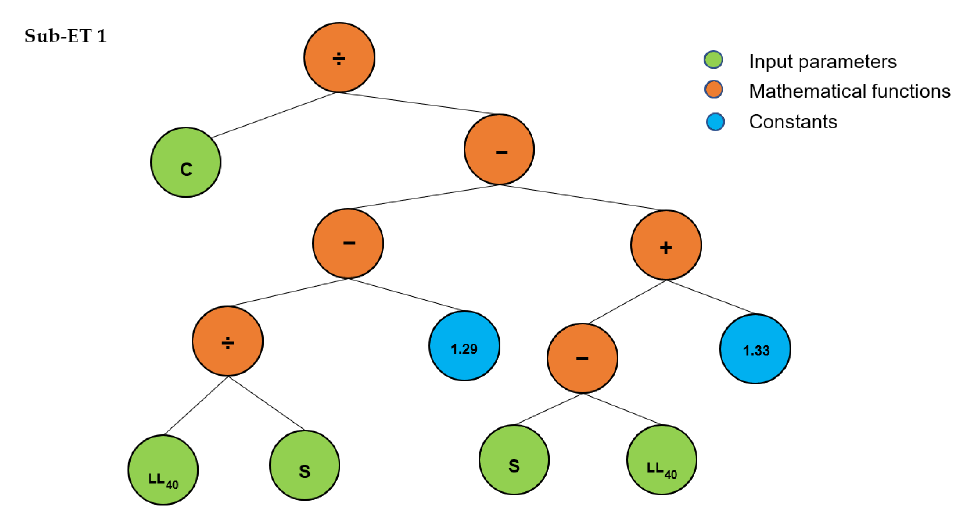
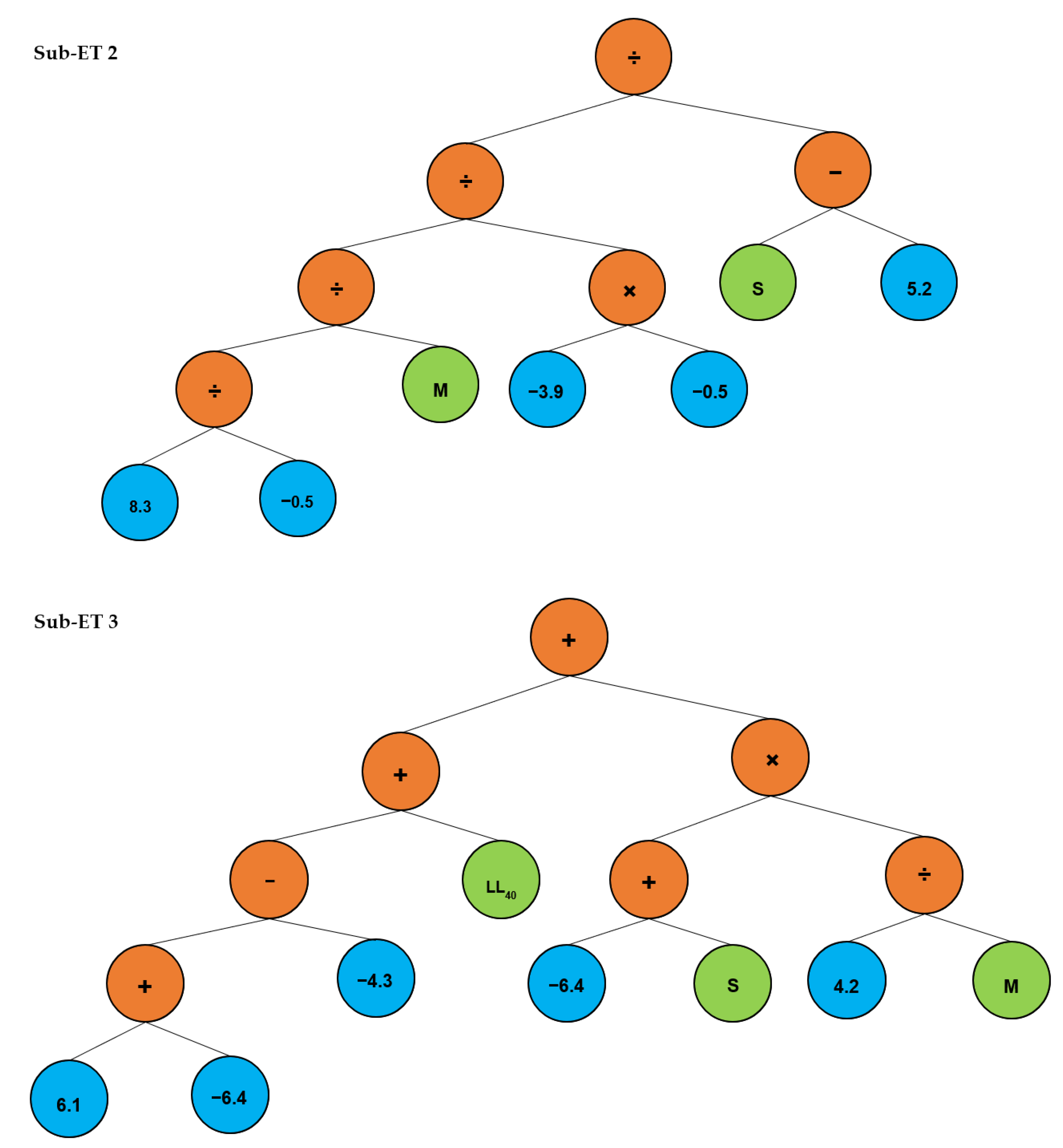
3. Development of Prediction Model Using Gene Expression Programming

After the compilation of data, a prediction model was developed using the AI-based technique. Gene expression programming (GEP) was chosen for this study because, in contrast to other data-science methodologies, it offers transparent solutions in the form of straightforward explicit mathematical equations and does not call for the prior assumption of correlations. For instance, an artificial neural network (ANN) is considered a “black box” and does not provide mathematical solutions. Similarly, simple multi-linear regression (MLR) does not give insights into the inter-dependency of variables.

GEP is the extended and improved version of GP, which was proposed by Ferreira and is widely appreciated by researchers in the field of geotechnical engineering [23,24,25,26,27,28]. Over the past few years, GEP has been adopted by many researchers in order to model complex physical phenomena. In GEP, chromosomes are expressed as branched structures also known as expression trees (ETs) of non-linear entities with varying sizes and shapes, which are initially encoded as fixed-size linear strings (genome). In a multi-genic chromosome, each gene represents Sub-ET, which is composed of two main parts; namely, head and tail. These are the positions where genetic operators are employed to develop new solutions. In GEP, a genetic code operator develops an optimal and best-fit solution of a complex problem in the form of empirical relations, which are formulated by linearly combining different input parameters and arithmetic operators (+, −, *, ÷, sine, cosine, tan, etc.) as a function set and constants as a terminal set. The information is stored in a chromosome, which is inferred using the Karwa language. Details in respect of the Karwa language can be found in the literature [29].

Figure 4 represents the process involved in developing an algorithm and explicit solution using GEP. The process begins with the random generation of an initial population for all the individuals. The chromosomes are expressed in the form of branched trees, i.e., ETs, and then best-fit solutions upon evaluation of fitness are used for the process of reproduction. The fitness can be evaluated using multiple functions and the notable examples are RMSE, MAE, RSE, and R². The iteration process is continued until the best desired optimal solution is obtained. Otherwise, the best-fit solution of the first iteration is selected using the Roulette wheel method and then the processes of mutation, crossover, and reproduction are applied to develop a new population of chromosomes. This process of iterations is stopped when best desired solution is obtained.

3.1. General Settings

The prediction model using GEP is controlled by the setting of general parameters such as the number of genes, head size, and the number of chromosomes [30,31,32]. Several trials were run to determine the optimal parameters for developing the algorithm. The experimental data obtained from 100 soil samples were used for the prediction model development by randomly distributing them into training and validation datasets in proportions of 70% and 30%, respectively. The head size, number of chromosomes, and genes were considered as 7, 30, and 3, respectively, in order to develop a robust solution for the problem at hand.

Table 2. General settings for the development of the prediction model.

General	Model Setting
	LL200 [%]
Genes	3
Chromosomes	30
Head size	7
Set of functions	+, −, ×, ÷
Linking function	+

shows the details of the setting of parameters involved in developing the GEP-based prediction model.

3.2. Prediction Model Evaluation Criteria

Prediction models are commonly evaluated using a single parameter known as a correlation coefficient. However, R cannot be solely contemplated as the measure to assess the performance and efficiency of the prediction model due to its insensitivity to division and multiplication of the output to a constant value. Therefore, root-mean-square error (RMSE), mean absolute error (MAE), and relatively squared error (RSE) were also considered in this study. These statistical parameters can be determined using Equations (2)–(5) [33].

$$\mathrm{RMSE}=\sqrt{\frac{{{\displaystyle \sum }}_{\mathrm{i}=1}^{\mathrm{n}}{\left({\mathrm{e}}_{\mathrm{i}}-{\mathrm{m}}_{\mathrm{i}}\right)}^2}{\mathrm{n}}}$$

(2)

$$\mathrm{MAE}=\frac{{{\displaystyle \sum }}_{\mathrm{i}=1}^{\mathrm{n}}\left({\mathrm{e}}_{\mathrm{i}}-{\mathrm{m}}_{\mathrm{i}}\right)}{\mathrm{n}}$$

(3)

$$\mathrm{RSE}=\frac{{{\displaystyle \sum }}_{\mathrm{i}=1}^{\mathrm{n}}{\left({\mathrm{m}}_{\mathrm{i}}-{\mathrm{e}}_{\mathrm{i}}\right)}^2}{{{\displaystyle \sum }}_{\mathrm{i}=1}^{\mathrm{n}}{\left(\stackrel{-}{\mathrm{e}}-{\mathrm{e}}_{\mathrm{i}}\right)}^2}$$

(4)

$$\mathrm{R}=\frac{{{\displaystyle \sum }}_{\mathrm{i}=1}^{\mathrm{n}}\left({\mathrm{e}}_{\mathrm{i}}-\overline{{\mathrm{e}}_{\mathrm{i}}}\right)\left({\mathrm{m}}_{\mathrm{i}}-\overline{{\mathrm{m}}_{\mathrm{i}}}\right)}{\sqrt{{{\displaystyle \sum }}_{\mathrm{i}=1}^{\mathrm{n}}{\left({\mathrm{e}}_{\mathrm{i}}-\overline{{\mathrm{e}}_{\mathrm{i}}}\right)}^2{{\displaystyle \sum }}_{\mathrm{i}=1}^{\mathrm{n}}{\left({\mathrm{m}}_{\mathrm{i}}-\overline{{\mathrm{m}}_{\mathrm{i}}}\right)}^2}}$$

(5)

where n is the number of samples, e_i is ith experimental output, m_i is the ith model output, and $\overline{{\mathrm{e}}_{\mathrm{i}}}$ and $\overline{{\mathrm{m}}_{\mathrm{i}}}$ are the average values of the experimental and the model responses, respectively.

The performance of prediction can also be evaluated using other statistical means as well as error plots. The prediction data that lie within the pre-defined error bounds represent the higher accuracy and generalization capability of the model [34]. Therefore, in this study, error plots were also drawn to ensure better insight into the accuracy of the proposed prediction models.

4. Results and Discussion

Figure 5 represents the ETs developed using GEP, which are composed of three sub-ETs (Sub-ET 1, sub-ET 2, and sub-ET 3). ETs were decoded according to the principles of the Karwa language, and the simplified expressions to predict LL₂₀₀ are given by Equations (6)–(9). The procedure involves the simple process of reading the expression tree from top to bottom and from left to right (exactly as we read a page of text). ETs are composed of three types of parameters such as constants (derived from iterative process of linear correlations to achieve a target value), input parameters, and pre-defined mathematical operators. It is evident from the mathematical expressions that the proposed model includes all the parameters that were involved in developing the model, accompanied by basic mathematical operators (+, −, * and ÷). These proposed mathematical models can be utilized explicitly and are more user-friendly for design engineers. The model is capable of quantifying the influence of different soil particles (S, C, and M), which can provide more insight to practitioners while performing design and analysis especially for the settlement analysis of foundations.

$${\mathrm{LL}}_{200} [\%]=A+B+C$$

(6)

$$A=\left[\frac{C}{\frac{{\mathrm{LL}}_{40}}{S}}-1.29\right]-\left[S-{\mathrm{LL}}_{40}+1.33\right]$$

(7)

$$B=\left[\left(\frac{44.2-8.5\times S}{M}\right)\right]$$

(8)

$$C=\left(4+{\mathrm{LL}}_{40}\right)+\left[\left(S-6.4\right)\left(\frac{4.2}{M}\right)\right]$$

(9)

where LL₂₀₀ (%) is the liquid limit based on # 200 sieve passing material; A, B, and C are the expressions derived from the three ETs; and LL₂₀₀ pis the summation of A, B, and C.

4.1. Performance Assessment of Model

The practical application of a prediction model depends upon how well the model meets the acceptance criteria. The model is deemed accurate and reliable if it satisfies multiple criteria. The performance evaluation criteria have been discussed in Section 3.2. Figure 6a represents the comparison of prediction data against the actual experimental data. The values of the statistical expressions are also shown in this graph. It can be seen that values of R², RMSE, MAE, and RSE are 0.985, 1.458, 1.165, and 0.014, respectively, for training data involved in training the prediction model, and are 0.983, 1.471, 1.207, and 0.018 for validation data. The values of R² close to 1 and lower values of RMSE, MAE, and RSE suggest strong predictability of the prediction equation [30]. This shows that the proposed prediction model complements all the acceptance criteria required to validate the performance of the prediction model as the values of R² are close to 1, i.e., 98% accuracy, whereas values of RMSE, MAE, and RSE are low enough for both training and validation datasets. Moreover, the training model performed well against unseen testing data that were not included in the development of the prediction model, with an accuracy of 98%. This further justifies that the proposed model predicts the responses with minimal error and high accuracy.

In addition to statistical checks, error plots also provide useful insights into the quantitative errors involved in predicting the responses using the trained model against unseen data. A model with minimal error is deemed reliable and accurate. In this regard, the proposed model was validated using several error plots. For example, Figure 6a also shows the plot of error bounds, and experimental and prediction responses. The results indicate that the experimental and predicted responses are well within the pre-defined error bounds such as ±5. It can be seen that the prediction data against actual experimental data lie within the +5% upper and −5% lower bounds, indicating the minimal error in prediction data. The frequencies of all the responses lie within ±5 error, indicating the high-performance efficiency of model.

4.2. Sensitivity and Parametric Study

Sensitivity analysis (SA) is carried out to determine the contributions of individual parameters involved in developing a prediction model. The sensitivity analysis indicates the sensitivity of a parameter in estimating the output. The most sensitive parameter must be dealt with carefully when it is determined in the laboratory or on site. The SA can be determined using Equation (10) [35,36]. The SA value varies between 1 and 0. The value of zero indicates that the parameter has no significant impact on the model output, whereas a value close to 1 shows the higher significance and level of sensitivity of the parameter.

$$SA=\frac{{{\displaystyle \sum }}_{\mathrm{i}=1}^{\mathrm{n}}\left(h_{\mathrm{i}}{k}_{\mathrm{i}}\right)}{\sqrt{{{\displaystyle \sum }}_{\mathrm{i}=1}^{\mathrm{n}}{h}_{\mathrm{i}}^{2}x {{\displaystyle \sum }}_1^{\mathrm{n}}{k}_{\mathrm{i}}^2}}$$

(10)

where h_i is the input parameter and k_i is the response of the predicted model.

Figure 7 shows the results of the sensitivity analysis for the proposed prediction model. It was observed that LL₄₀ has the most significant impact, followed by C, M, and S. The determination of LL₄₀ has a considerable effect on estimating LL₂₀₀ and it must be treated with utmost care in a laboratory. The order of significance is LL₄₀ > C > M > S. C is the most significant soil property that influences the Atterberg limits and similar findings have been reported in the literature [37]. S is the least sensitive parameter. Nevertheless, the value of SA for S is the least among all parameters, but it does not necessarily follow that the impact of S on LL₂₀₀ would be negligible as it has 78% sensitivity, which indicates its higher sensitivity in relation to LL₂₀₀. This translates to the fact that the model has been trained effectively since all the parameters considered for developing the model have a significant impact on LL₂₀₀.

The development of prediction models brings robust and cost-effective solutions using state-of-the-art knowledge. However, the models present several challenges to be addressed before their consideration for wider applicability. Some models are trained effectively and are solely based on the data utilized in the developing model. AI-based techniques cannot assess whether the data utilized justify physical processes or not. In this regard, parametric studies were conducted as shown in Figure 8. In this process, all the input parameters are kept constant at their average values while one parameter is varied around its mean value, and the corresponding variation in the dependent parameter is observed. It can be seen that an increase in LL₄₀ leads to an increase in LL₂₀₀, which is because finer particles tend to have a larger surface area and this consequently leads to an increase in the liquid limit with particle sizes smaller than 0.075 mm (# 200 sieve). Similarly, increases in C and M lead to an increase in LL₂₀₀; it has been discussed in several research studies that an increase in C leads to an increase in the water holding capacity of soils [1,12,37]. Similarly, an increase in M causes an increase in LL₂₀₀ as M particles have a small size and can enhance the LL due to the larger surface area. Variation of the most critical parameters has been considered for the sake of brevity. These findings demonstrate that the model meets all the requirements for prediction model acceptance and may be applied in practice with greater accuracy.

4.3. Practical Application and Future Prospects of Research

As discussed, the liquid limit is the most fundamental parameter that is commonly used for the design and analysis of many geotechnical applications. One of the prime examples is that it is employed for the settlement analysis of foundations and plays key role in the classification of soils, leading to selection of material for the construction of roads and backfill. The LL depends upon several factors such as particle sizes, type of clay minerals (montmorillonite, illite, kaolinite etc.), cation exchange capacity (CEC), pH, and so on. Conventional methods do not incorporate the effect of critical influencing parameters and have certain limitations, which have already been discussed. Thus, the proposed prediction model considers the most easily available critical parameters controlling the LL of soil by proposing user-friendly stochastic expression. The suggested approach offers helpful insights into how particle sizes affect LL determination, which ultimately results in effective material selection based on accurate soil-type categorization and safe design of construction. However, because of the attributes of the dataset used for model construction, this model is better suited to low-plasticity silty clayey types of soils. Future research may be conducted on the diverse nature of clayey soils (highly reactive, expansive, and dispersive soils) incorporating a micro-structure study of clayey particles and several other parameters, such as the cation exchange capacity of clayey soil and pH. The concept of determining the LL based on # 200 sieve passing may also be implemented to revise existing correlations of LL₄₀ with the mechanical properties of soil.

5. Conclusions

In this study we proposed a novel AI-based prediction model for the liquid limit based on material having a size smaller than 0.075 mm, using the GEP technique. The proposed empirical model is the first of its kind and can be implemented in the field when provided with known values of sand content, silt content, clay content, and liquid limit using # 40 sieve passing material. The following principal conclusions can be drawn from this study.

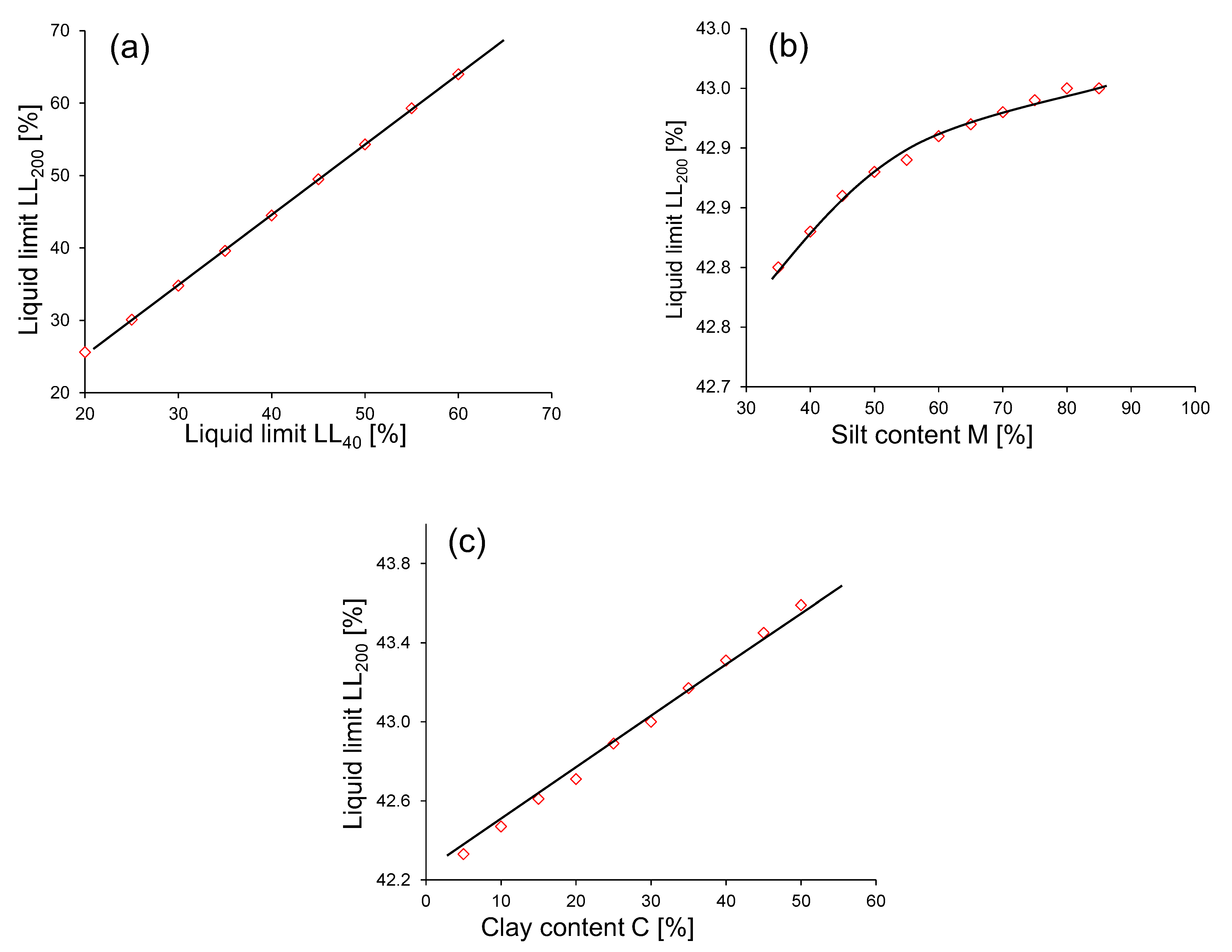
• The LL is governed by different particle sizes, which include S, C, and M. However, conventional methods do not incorporate the effect of S, C, and M explicitly. Therefore, the proposed model was developed to account for S, C, and M in order to better capture the behavior of the consistency of fine soils.
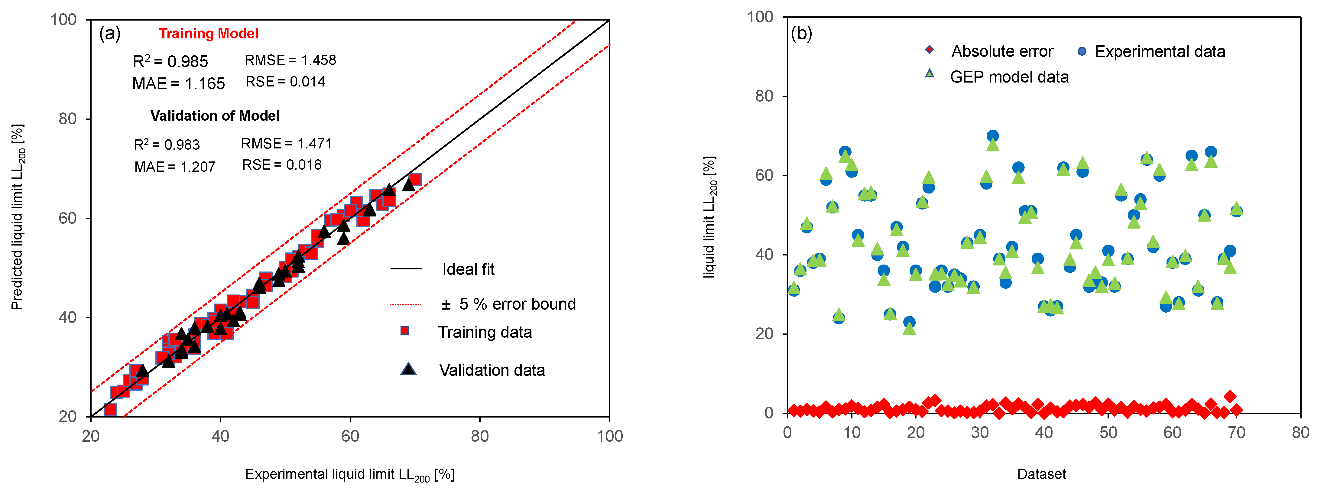
• The proposed prediction model is simple, robust, and justifies all the acceptance requirements in terms of high accuracy and low errors in prediction. The values of R², RMSE, MAE, and RSE for training data were found to be 0.985, 1.458, 1.165, and 0.014, respectively, and were 0.983, 1.471, 1.207, and 0.018 for validation data. The results indicate the higher accuracy and generalization capability of the proposed prediction model.
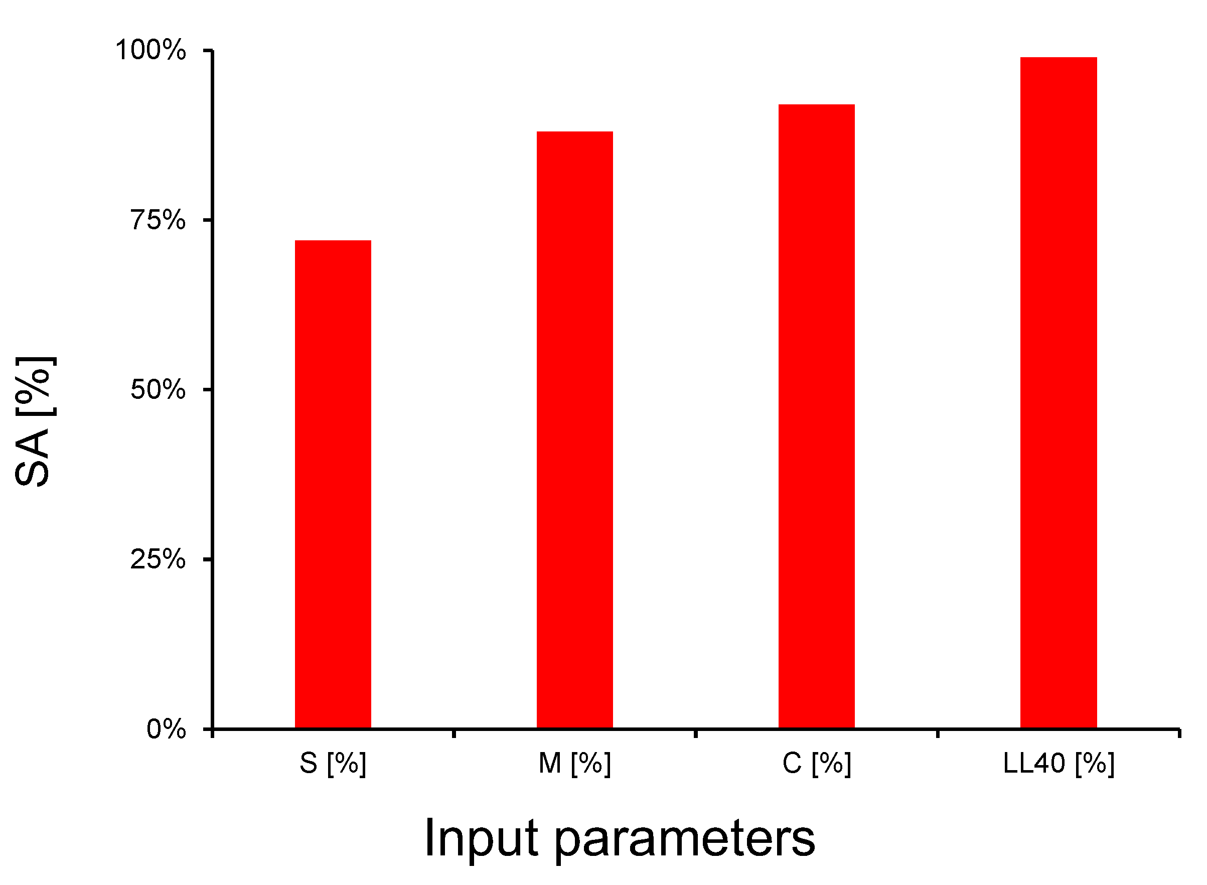
• The proposed model predicted the responses with minimal error and the prediction data lie within ±5% error, which further confirms the reliability. The performance of the sensitivity analysis indicates that all the parameters involved in developing the model are sensitive to LL₂₀₀, with S being the least significant parameter and having a sensitivity value of 0.78.
• The model can be used with the least possible error for low-plasticity clayey soils and reduces the risk of underestimation of the LL, eventually leading to the safe design and analysis of structures.

References

1. Das, B.M. Principles of Geotechnical Engineering; Cengage Learning: Belmont, CA, USA, 2021; ISBN 0357420667. [Google Scholar]
2. Bowles, J.E. Foundation Engineering; McGraw Hills: Singapore, 1997. [Google Scholar]
3. Sharma, B.; Bora, P.K. Plastic Limit, Liquid Limit and Undrained Shear Strength of Soil—Reappraisal. J. Geotech. Geoenvironment. Eng. 2003, 129, 774–777. [Google Scholar] [CrossRef]
4. Haigh, S. Consistency of the Casagrande Liquid Limit Test. Geotech. Test. J. 2015, 39. [Google Scholar] [CrossRef]
5. Budhu, M. Soil Mechanics and Foundations; John Wiley & Sons: Hoboken, NJ, USA, 2010; ISBN 0470556846. [Google Scholar]
6. Casey, B.; Germaine, J.T. Stress Dependence of Shear Strength in Fine-Grained Soils and Correlations with Liquid Limit. J. Geotech. Geoenviron. Eng. 2013, 139, 1709–1717. [Google Scholar] [CrossRef]
7. ASTM-D4318; Test Methods for Liquid Limit, Plastic Limit, and Plasticity Index of Soils. ASTM: West Conshohocken, PA, USA, 2017. [CrossRef]
8. BS 1377-2:2022; Methods of Test for Soils for Civil Engineering Purpose. Part 2: Classification Tests. BSI: London, UK, 1990.
9. Stevens, J. Unified Soil Classification System. Civ. Eng. ASCE 1982, 52, 61–62. [Google Scholar]
10. Polidori, E. Proposal for a New Classification of Common Inorganic Soils for Engineering Purposes. Geotech. Geol. Eng. 2015, 33, 1569–1579. [Google Scholar] [CrossRef]
11. Polidori, E. Relationship between the Atterberg Limits and Clay Content. Soils Found. 2007, 47, 887–896. [Google Scholar] [CrossRef]
12. Afolagboye, L.; Abdu-Raheem, Y.A.; Ajayi, D.E.; Talabi, A.O. A Comparison between the Consistency Limits of Lateritic Soil Fractions Passing through Sieve Numbers 40 and 200. Innov. Infrastruct. Solut. 2021, 6, 1–8. [Google Scholar] [CrossRef]
13. Mousavi, S.M.; Alavi, A.H.; Gandomi, A.H.; Mollahasani, A. Nonlinear Genetic-Based Simulation of Soil Shear Strength Parameters. J. Earth Syst. Sci. 2011, 120, 1001–1022. [Google Scholar] [CrossRef]
14. Mousavi, S.M.; Alavi, A.H.; Mollahasani, A.; Gandomi, A.H. A Hybrid Computational Approach to Formulate Soil Deformation Moduli Obtained from PLT. Eng. Geol. 2011, 123, 324–332. [Google Scholar] [CrossRef]
15. Zheng, D.; Wu, R.; Sufian, M.; Kahla, N.B.; Atig, M.; Deifalla, A.F.; Accouche, O.; Azab, M. Flexural Strength Prediction of Steel Fiber-Reinforced Concrete Using Artificial Intelligence. Materials 2022, 15, 5194. [Google Scholar] [CrossRef]
16. Shah, S.A.R.; Azab, M.; Seif ElDin, H.M.; Barakat, O.; Anwar, M.K.; Bashir, Y. Predicting Compressive Strength of Blast Furnace Slag and Fly Ash Based Sustainable Concrete Using Machine Learning Techniques: An Application of Advanced Decision-Making Approaches. Buildings 2022, 12, 914. [Google Scholar] [CrossRef]
17. Seybold, C.A.; Elrashidi, M.A.; Engel, R.J. Linear Regression Models to Estimate Soil Liquid Limit and Plasticity Index from Basic Soil Properties. Soil Sci. 2008, 173, 25–34. [Google Scholar] [CrossRef]
18. Díaz, E.; Pastor, J.L.; Rabat, Á.; Tomás, R. Machine Learning Techniques for Relating Liquid Limit Obtained by Casagrande Cup and Fall Cone Test in Low-Medium Plasticity Fine Grained Soils. Eng. Geol. 2021, 294, 106381. [Google Scholar] [CrossRef]
19. Keller, T.; Dexter, A.R. Plastic Limits of Agricultural Soils as Functions of Soil Texture and Organic Matter Content. Soil Res. 2012, 50, 7–17. [Google Scholar] [CrossRef]
20. Karakan, E.; Shimobe, S.; Sezer, A. Effect of Clay Fraction and Mineralogy on Fall Cone Results of Clay–Sand Mixtures. Eng. Geol. 2020, 279, 105887. [Google Scholar] [CrossRef]
21. Wroth, C.P.; Wood, D.M. The Correlation of Index Properties with Some Basic Engineering Properties of Soils. Can. Geotech. J. 1978, 15, 137–145. [Google Scholar] [CrossRef]
22. ASTM D6913/D6913M-17; Standard Test Method for Particle-Size Analysis of Soils. ANSI: Washington, DC, USA, 2007.
23. Ferreira, C. Gene Expression Programming: Mathematical Modeling by an Artificial Intelligence; Springer: Berlin/Heidelberg, Germany, 2006; Volume 21, ISBN 3540328491. [Google Scholar]
24. Al Bodour, W.; Hanandeh, S.; Hajij, M.; Murad, Y. Development of Evaluation Framework for the Unconfined Compressive Strength of Soils Based on the Fundamental Soil Parameters Using Gene Expression Programming and Deep Learning Methods. J. Mater. Civ. Eng. 2022, 34, 4021452. [Google Scholar] [CrossRef]
25. Mollahasani, A.; Alavi, A.H.; Gandomi, A.H. Empirical Modeling of Plate Load Test Moduli of Soil via Gene Expression Programming. Comput. Geotech. 2011, 38, 281–286. [Google Scholar] [CrossRef]
26. Azim, I.; Yang, J.; Javed, M.F.; Iqbal, M.F.; Mahmood, Z.; Wang, F.; Liu, Q. Prediction Model for Compressive Arch Action Capacity of RC Frame Structures under Column Removal Scenario Using Gene Expression Programming. In Structures; Elsevier: Amsterdam, The Netherlands, 2020; Volume 25, pp. 212–228. [Google Scholar]
27. Tarawneh, B. Gene Expression Programming Model to Predict Driven Pipe Piles Set-Up. Int. J. Geotech. Eng. 2018, 14, 538–544. [Google Scholar] [CrossRef]
28. Pham, V.-N.; Oh, E.; Ong, D.E.L. Effects of Binder Types and Other Significant Variables on the Unconfined Compressive Strength of Chemical-Stabilized Clayey Soil Using Gene-Expression Programming. Neural Comput. Appl. 2022, 34, 9103–9121. [Google Scholar] [CrossRef]
29. Ferreira, C. Gene Expression Programming in Problem Solving. In Soft Computing and Industry; Springer: Berlin/Heidelberg, Germany, 2002; pp. 635–653. [Google Scholar]
30. Iqbal, M.F.; Liu, Q.; Azim, I.; Zhu, X.; Yang, J.; Javed, M.F.; Rauf, M. Prediction of Mechanical Properties of Green Concrete Incorporating Waste Foundry Sand Based on Gene Expression Programming. J. Hazard. Mater. 2020, 384, 121322. [Google Scholar] [CrossRef] [PubMed]
31. Çanakcı, H.; Baykasoğlu, A.; Güllü, H. Prediction of Compressive and Tensile Strength of Gaziantep Basalts via Neural Networks and Gene Expression Programming. Neural Comput. Appl. 2009, 18, 1031–1041. [Google Scholar] [CrossRef]
32. Goharzay, M.; Noorzad, A.; Ardakani, A.M.; Jalal, M. A Worldwide SPT-Based Soil Liquefaction Triggering Analysis Utilizing Gene Expression Programming and Bayesian Probabilistic Method. J. Rock Mech. Geotech. Eng. 2017, 9, 683–693. [Google Scholar] [CrossRef]
33. Gholampour, A.; Gandomi, A.H.; Ozbakkaloglu, T. New Formulations for Mechanical Properties of Recycled Aggregate Concrete Using Gene Expression Programming. Constr. Build. Mater. 2017, 130, 122–145. [Google Scholar] [CrossRef]
34. Hassan, J.; Alshameri, B.; Iqbal, F. Prediction of California Bearing Ratio (CBR) Using Index Soil Properties and Compaction Parameters of Low Plastic Fine-Grained Soil. Transp. Infrastruct. Geotechnol. 2021, 1–13. [Google Scholar] [CrossRef]
35. Wang, H.-L.; Yin, Z.-Y. High Performance Prediction of Soil Compaction Parameters Using Multi Expression Programming. Eng. Geol. 2020, 276, 105758. [Google Scholar] [CrossRef]
36. Ardakani, A.; Kordnaeij, A. Soil Compaction Parameters Prediction Using GMDH-Type Neural Network and Genetic Algorithm. Eur. J. Environ. Civ. Eng. 2019, 23, 449–462. [Google Scholar] [CrossRef]
37. Zolfaghari, Z.; Mosaddeghi, M.R.; Ayoubi, S. ANN-based Pedotransfer and Soil Spatial Prediction Functions for Predicting Atterberg Consistency Limits and Indices from Easily Available Properties at the Watershed Scale in Western Iran. Soil Use Manag. 2015, 31, 142–154. [Google Scholar] [CrossRef]
Figure 1. Steps involved in developing prediction model using artificial intelligence techniques.
Buildings 12 01551 g001
Figure 2. Location map of the soil study area.
Buildings 12 01551 g002
Figure 3. Frequency distribution histograms of experimental data: (a) sand content S [%]; (b) silt content M [%]; (c) clay content C [%]; (d) liquid limit from # 40 sieve passing material LL40 [%]; (e) liquid limit from # 200 sieve passing material LL200 [%].
Buildings 12 01551 g003aBuildings 12 01551 g003b
Figure 4. Steps involved in developing the algorithm of GEP.
Buildings 12 01551 g004
Figure 5. Expression trees [ETs] were developed using gene expression programming [GEP].
Buildings 12 01551 g005aBuildings 12 01551 g005b
Figure 6. Performance evaluation of prediction model of LL200: (a) statistical analysis of proposed prediction model of LL200; (b) comparison of GEP model responses, experimental data, and absolute error.
Buildings 12 01551 g006
Figure 7. Sensitivity analysis of prediction model based on sensitivity of individual input parameters.
Buildings 12 01551 g007
Figure 8. Parametric analysis of input parameters; (a) variation of liquid limit LL200 with varying liquid limit based on # 40 sieve passing material [%]; (b) variation of liquid limit LL200 with varying silt content M [%]; (c) variation of liquid limit LL200 with varying clay content C [%].
Buildings 12 01551 g008