
Research on Optimization of Climate Responsive Indoor Space Design in Residential Buildings


Abstract
:1. Introduction
2. Background and Literature
2.1. Literature Review
2.1.1. Building Climate Responsive Design
2.1.2. Multi-Objective Optimization
Subject to: gi(X) ≤ 0, i = 1, 2, …, m
Kj(X) = 0, j = 1, 2, …, p
2.1.3. Research Gap
- Transition from energy-saving design practice or theoretical research based on qualitative analysis to quantitative research based on energy consumption simulation.
- The research related to building energy consumption is becoming more and more comprehensive, from only focusing on the thermal performance of buildings or the energy consumption of heating and cooling systems to comprehensive assessments that also consider other factors such as total building energy consumption, lighting and indoor thermal comfort.
- “Performance coupling factors” are valued. The development of society and economy requires sustainable building design to achieve low energy consumption under the premise of ensuring high performance building environment, and “high performance” cannot be sacrificed for low energy consumption. As the pursuit of single-environment performance improvement often has an adverse effect on other aspects of performance, research on multiple environments and their coupling performance has attracted more and more attention.
- New tools or new methods for building performance simulation such as BIM technology or computer programming technology are constantly emerging. On this basis, the amount of simulated data is increasing and the reliability of simulation results is improving.
2.2. Typical Cities’ Selection
3. Multi-Objective Model Set-Up
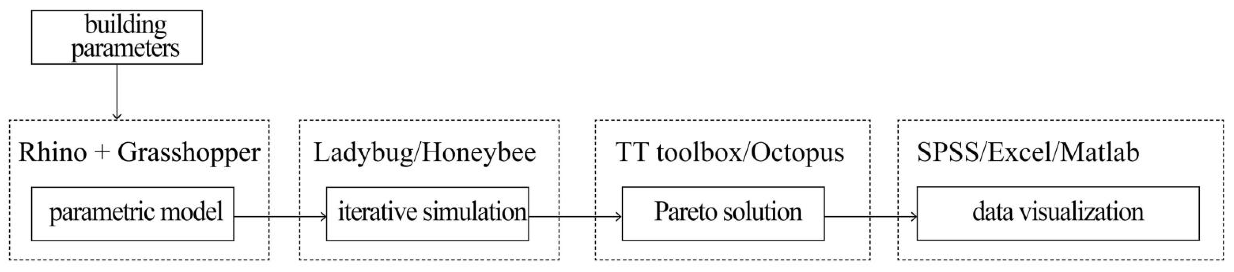
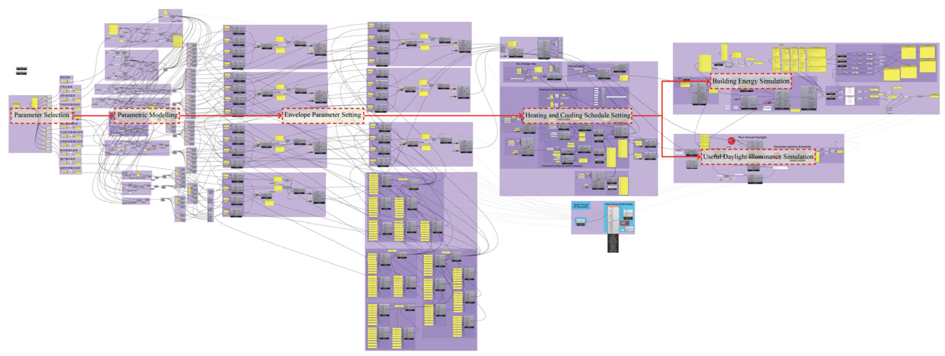
3.1. Building Performance Optimization Workflow
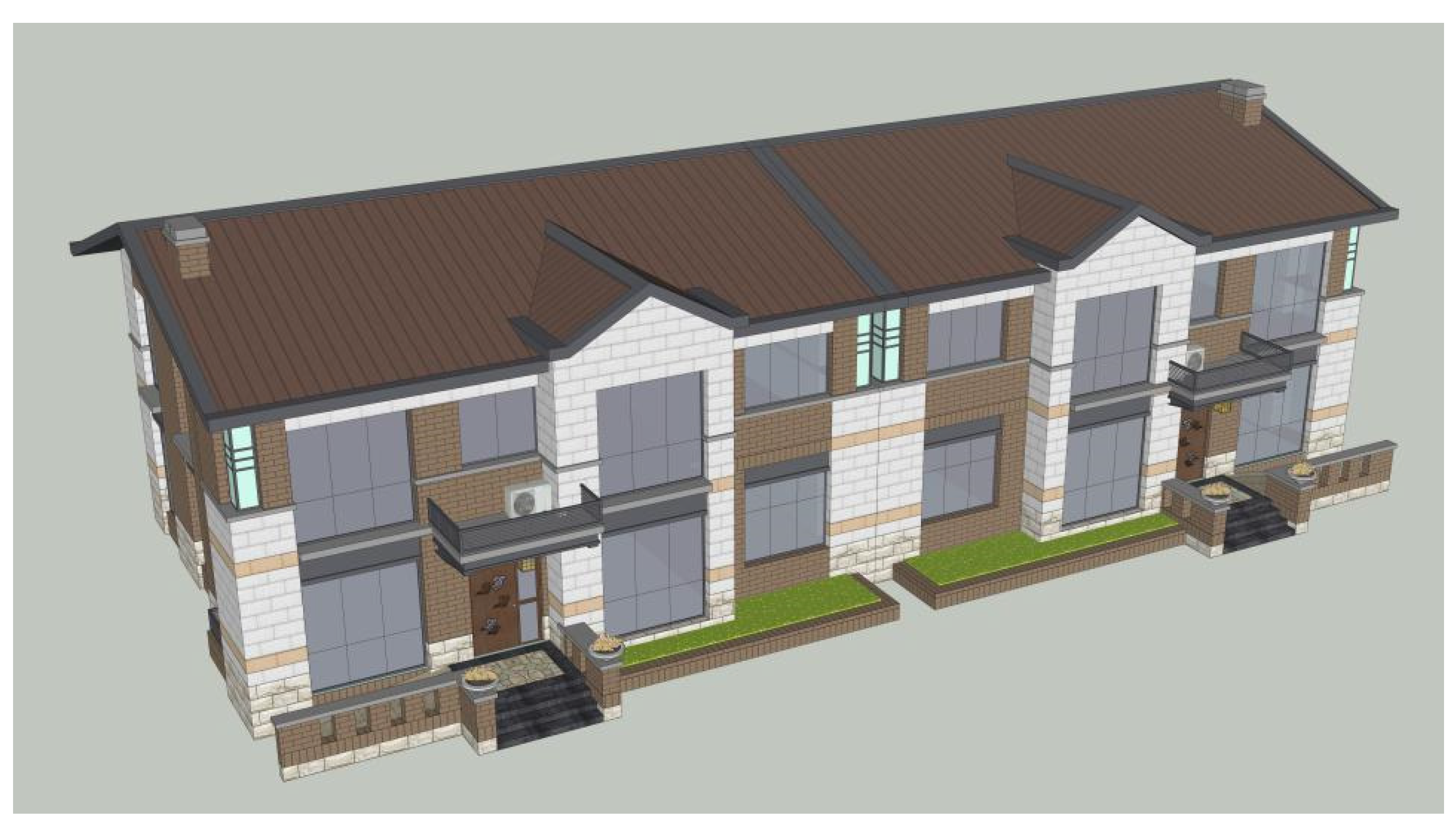
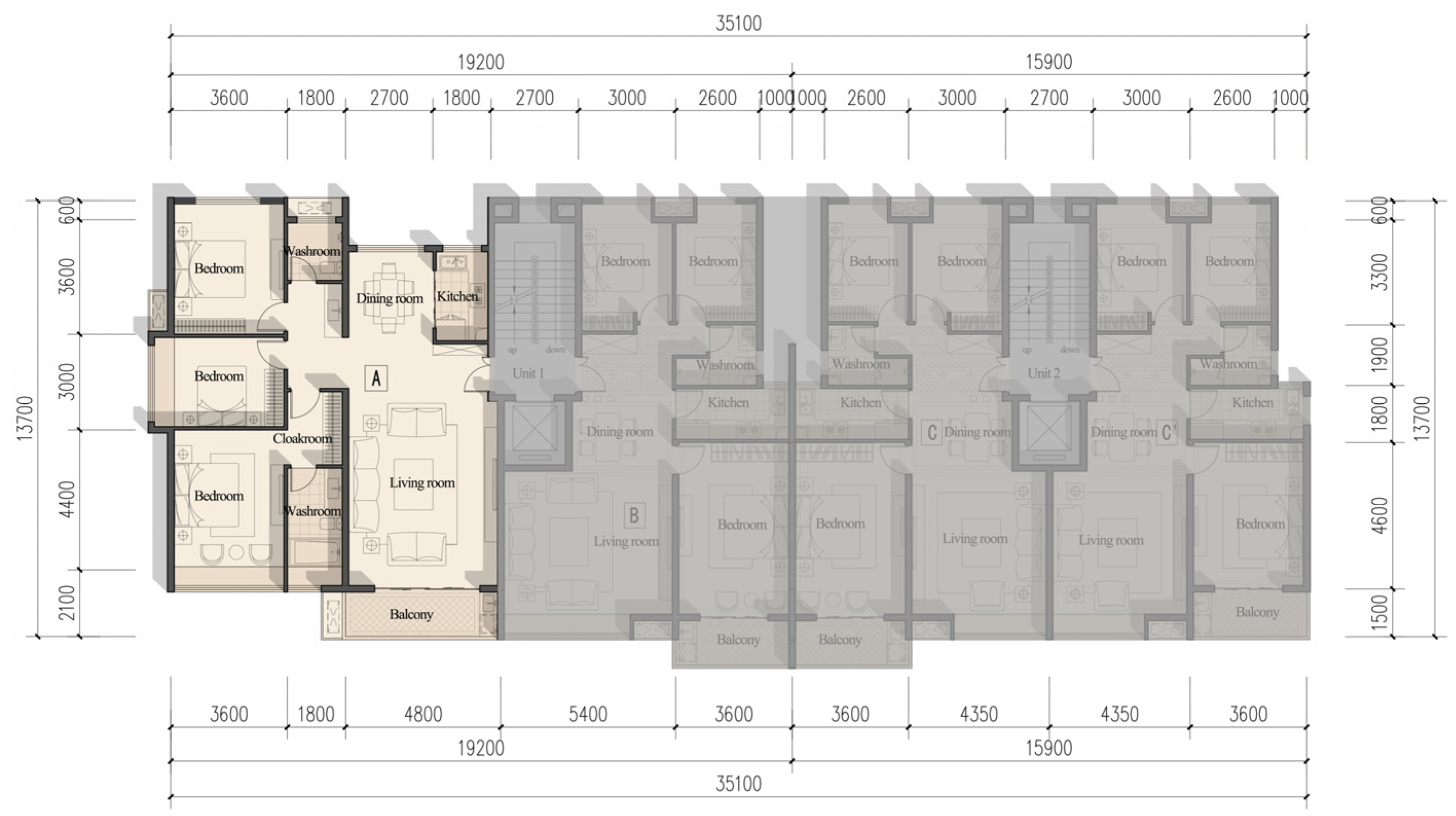
3.2. Building Parameter Settings
= Kitchen/Dining room depth + Living room depth
= Total depth
= Northern bedroom width + 1.8 m (Toilet width) + Dining room width + Kitchen width
= Total width
3.3. Objective Function Settings
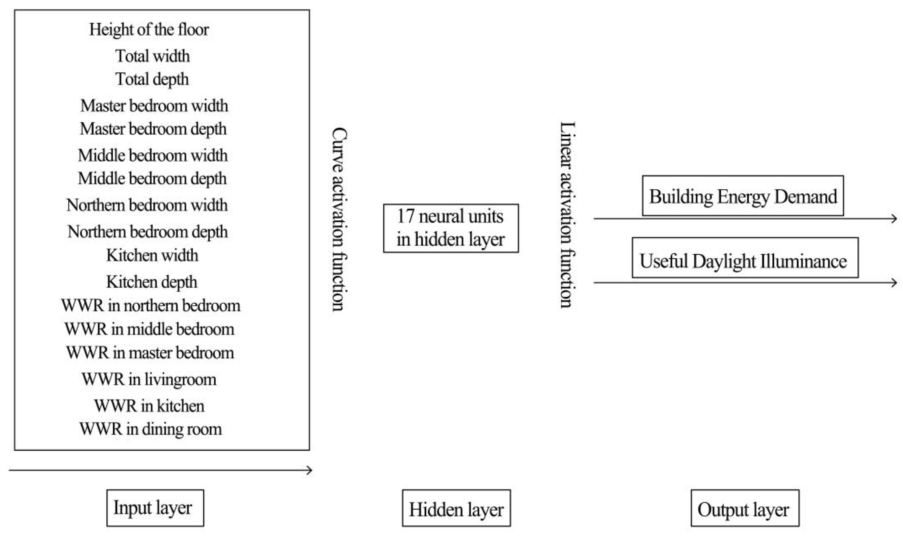
3.3.1. Building Energy Demand
3.3.2. Lighting Environment Comfort
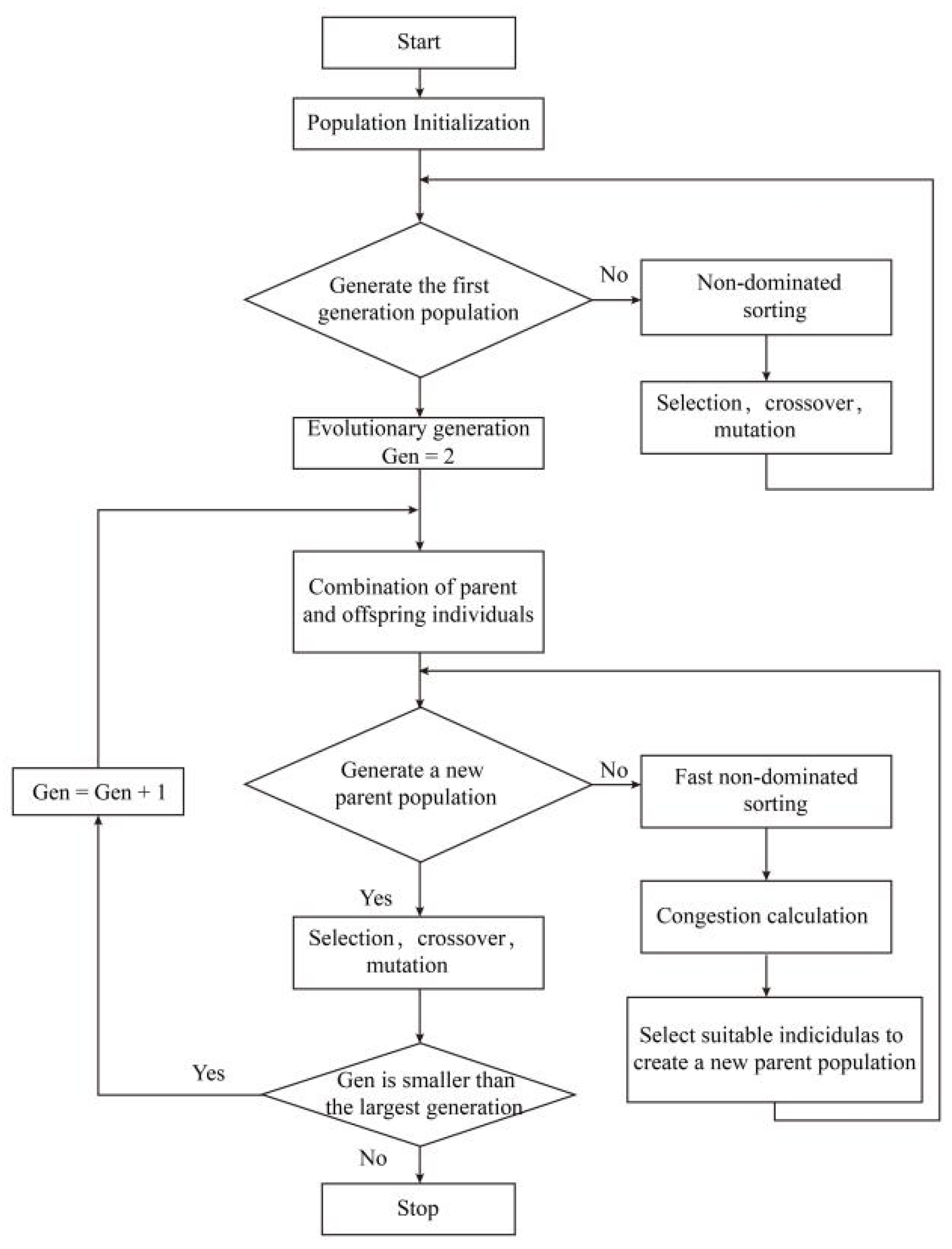
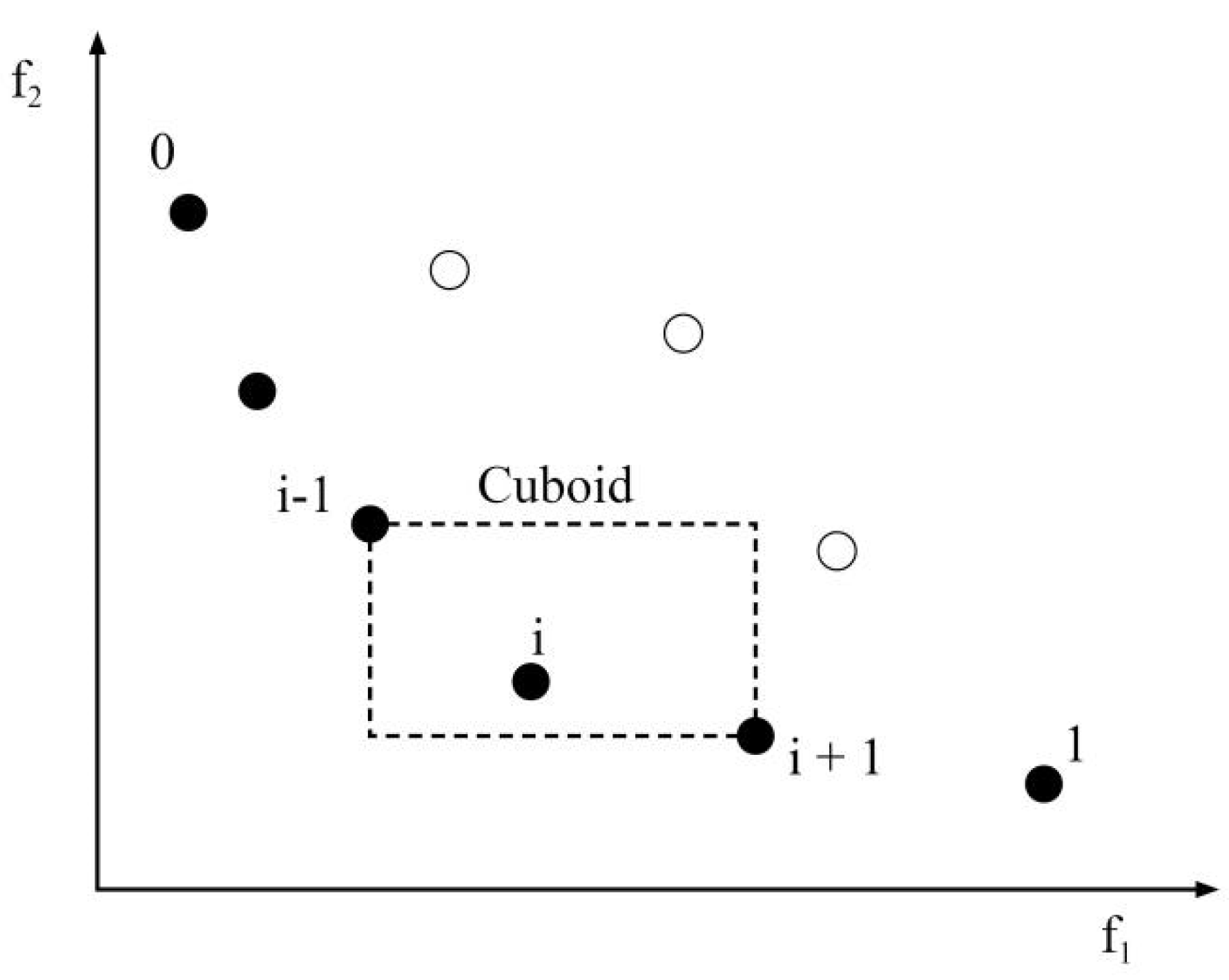
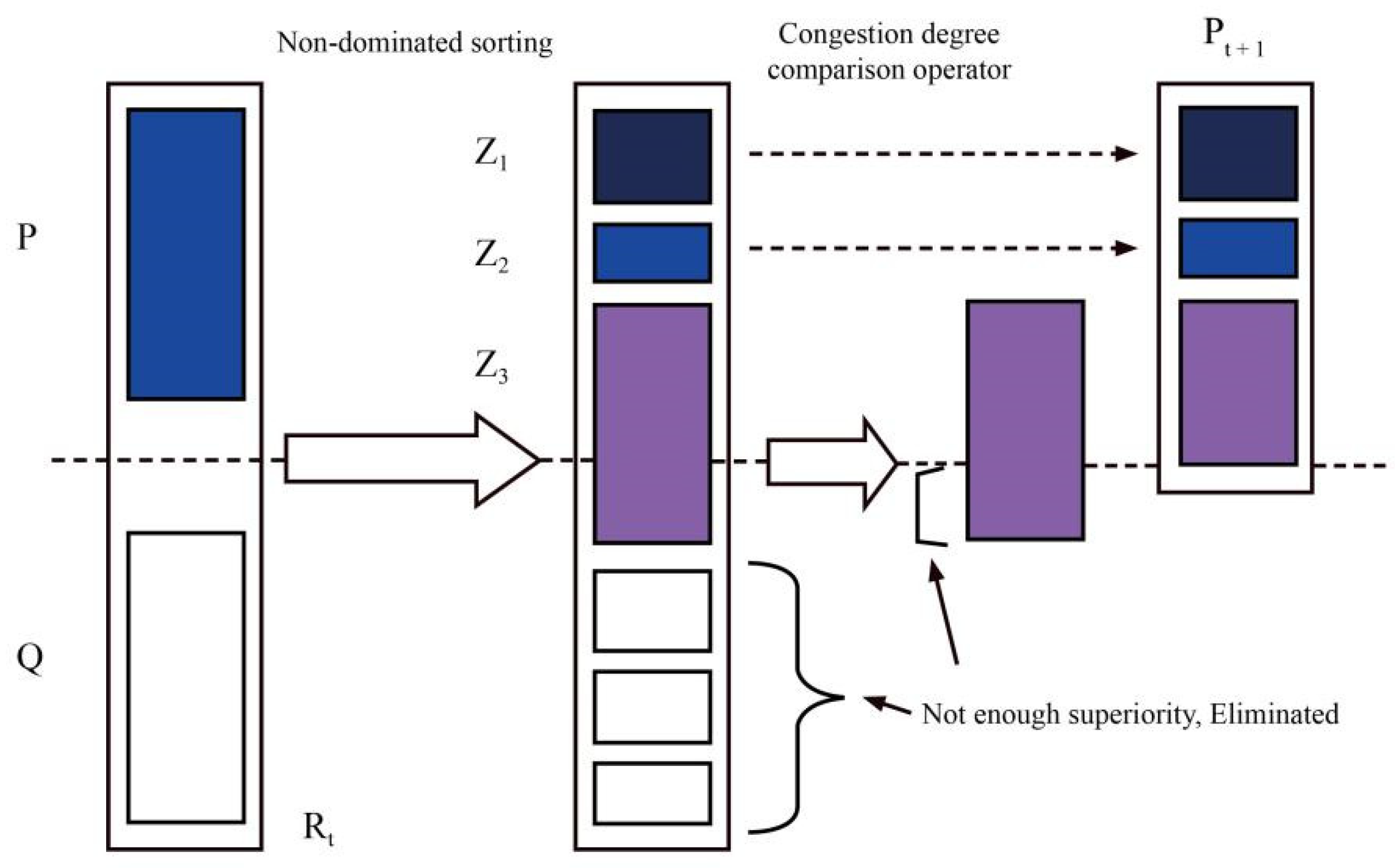
3.4. Multi-Objective Optimization Algorithm
- (1)
- Let nd = 0, n = 1, 2, …, N
- (2)
- For each objective function
- The population was ranked based on the objective function,
- Let the crowding degree of two individuals on the boundary be infinite, that is, ld = nd = ∞,
- Calculate nd = nd + (ƒm(i + 1) − ƒm(i − 1)), n = 2, 3, …, N − 1
- (1)
- If irank < jrank
- (2)
- If they have the same rank and individual i has a larger crowding distance than individual j, i.e., irank = jrank and id > jd
4. Predictive Model Set-Up and Sensitivity Analysis
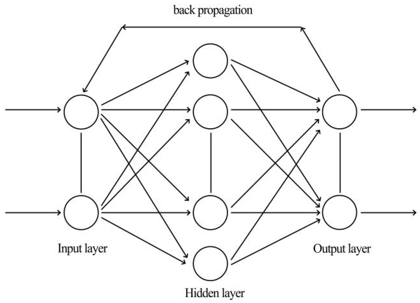
4.1. Artificial Neural Network Theory
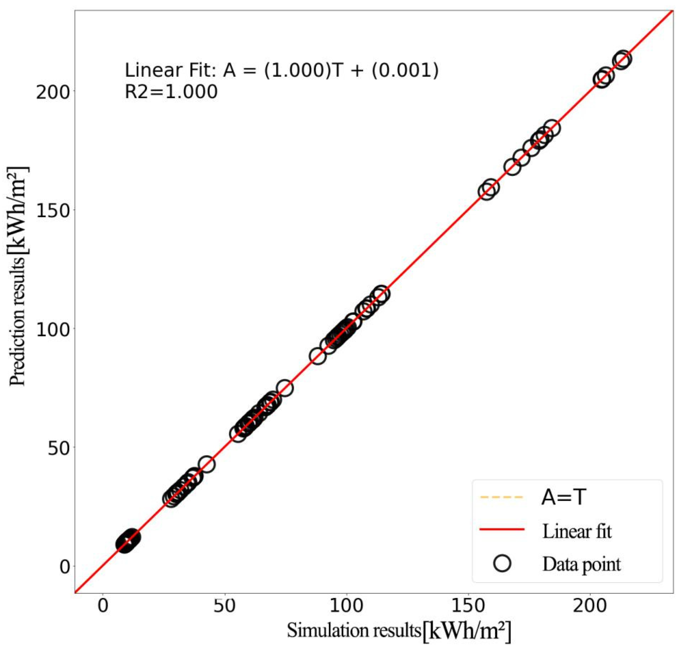
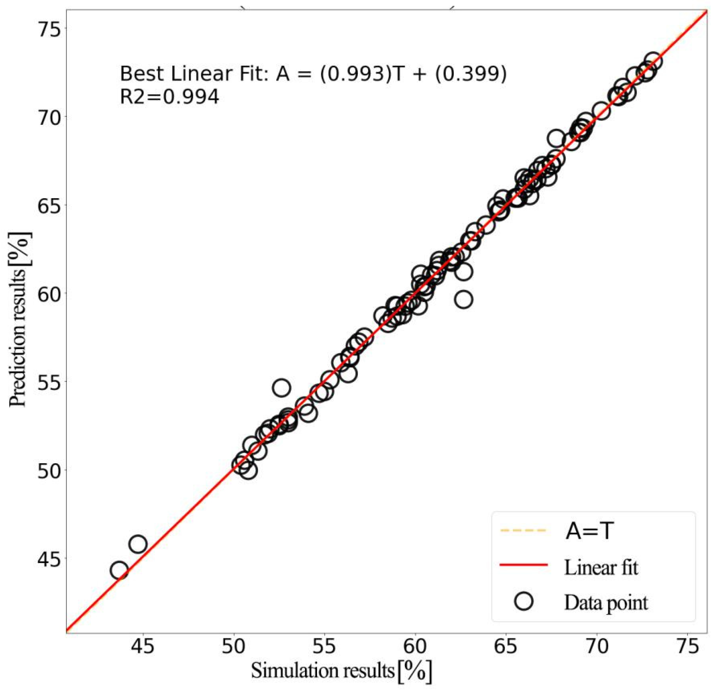
4.2. Prediction Model Set-Up for Residential Building Simulation in Typical Cities
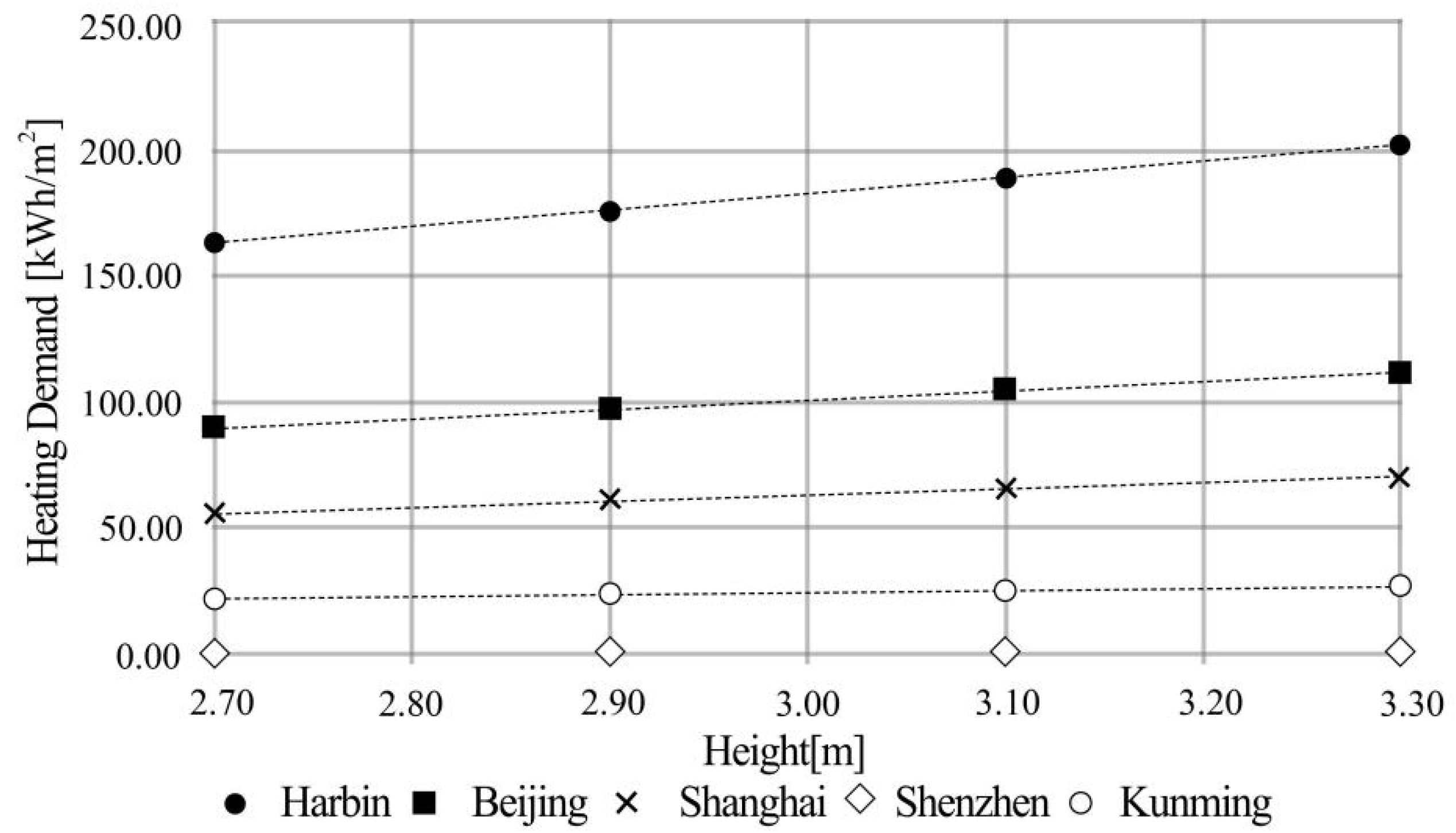
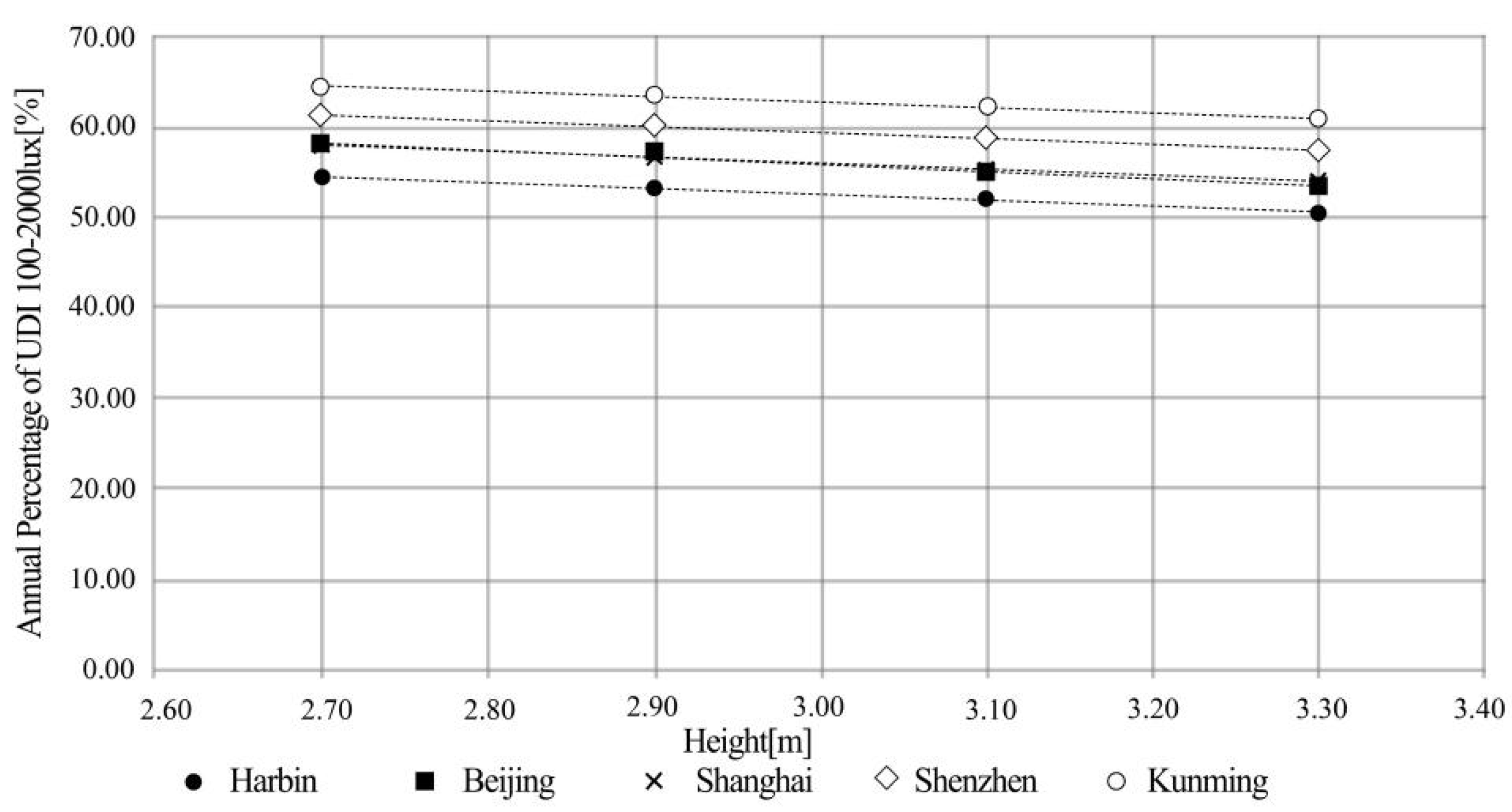
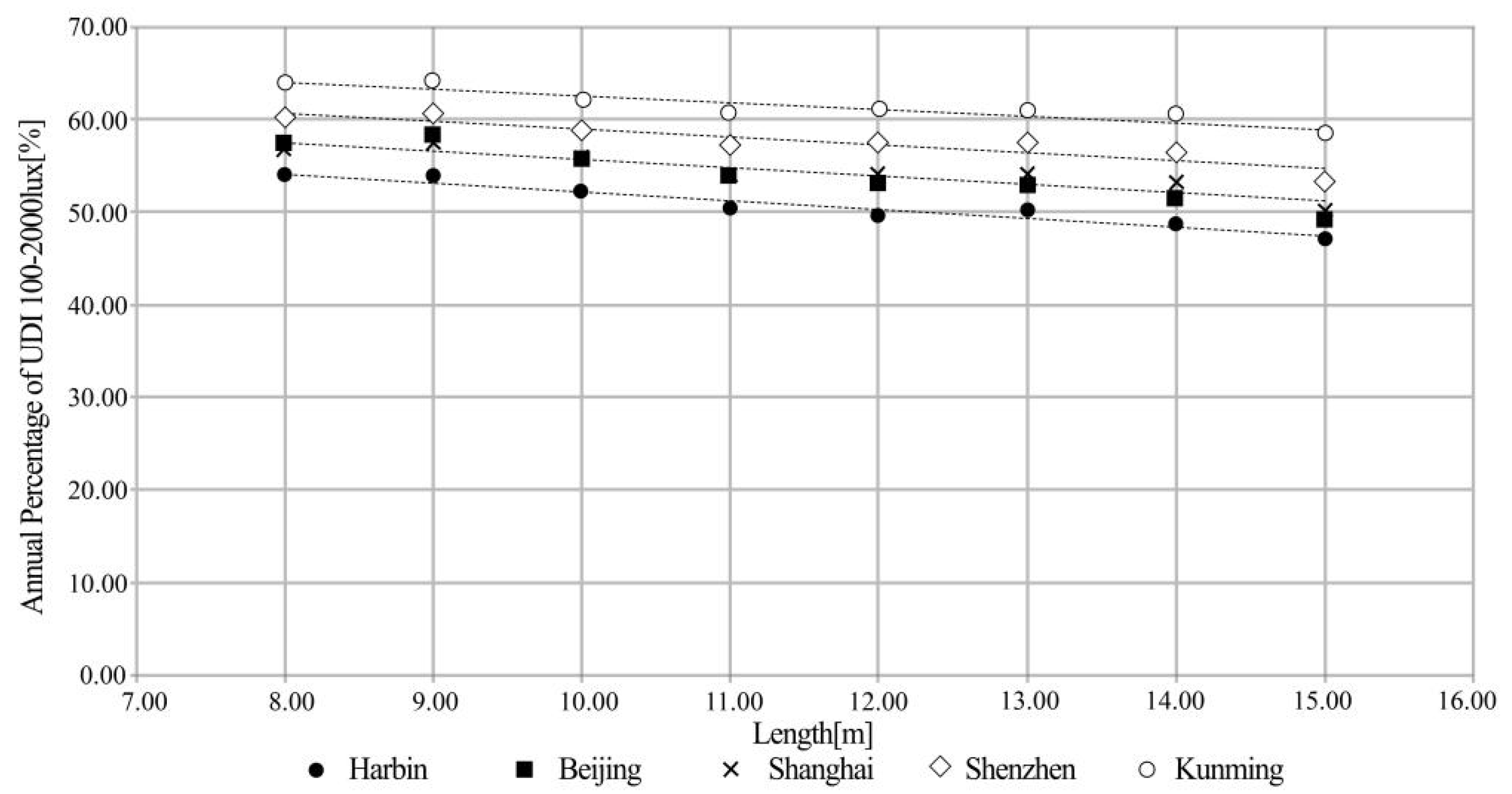
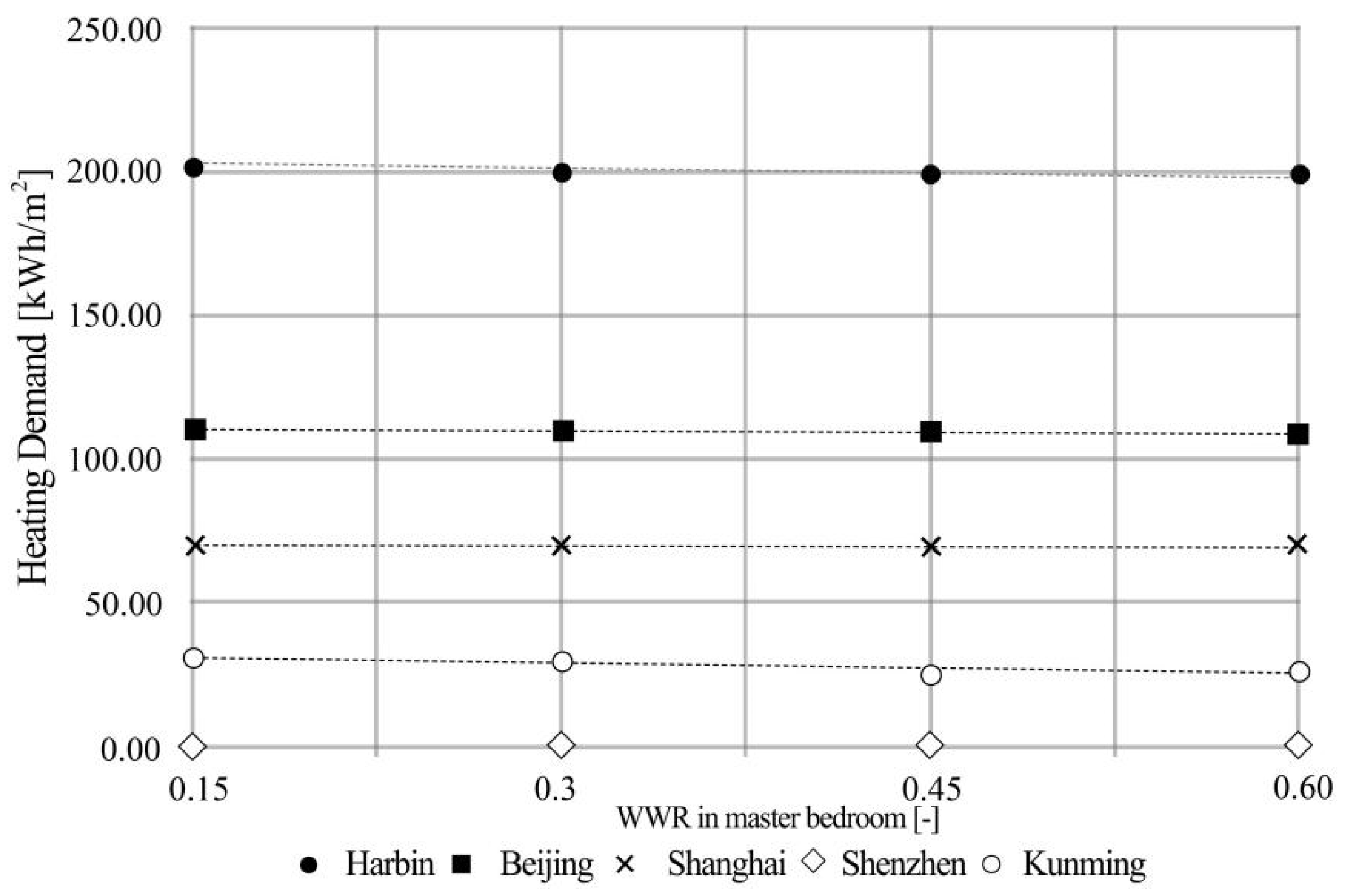
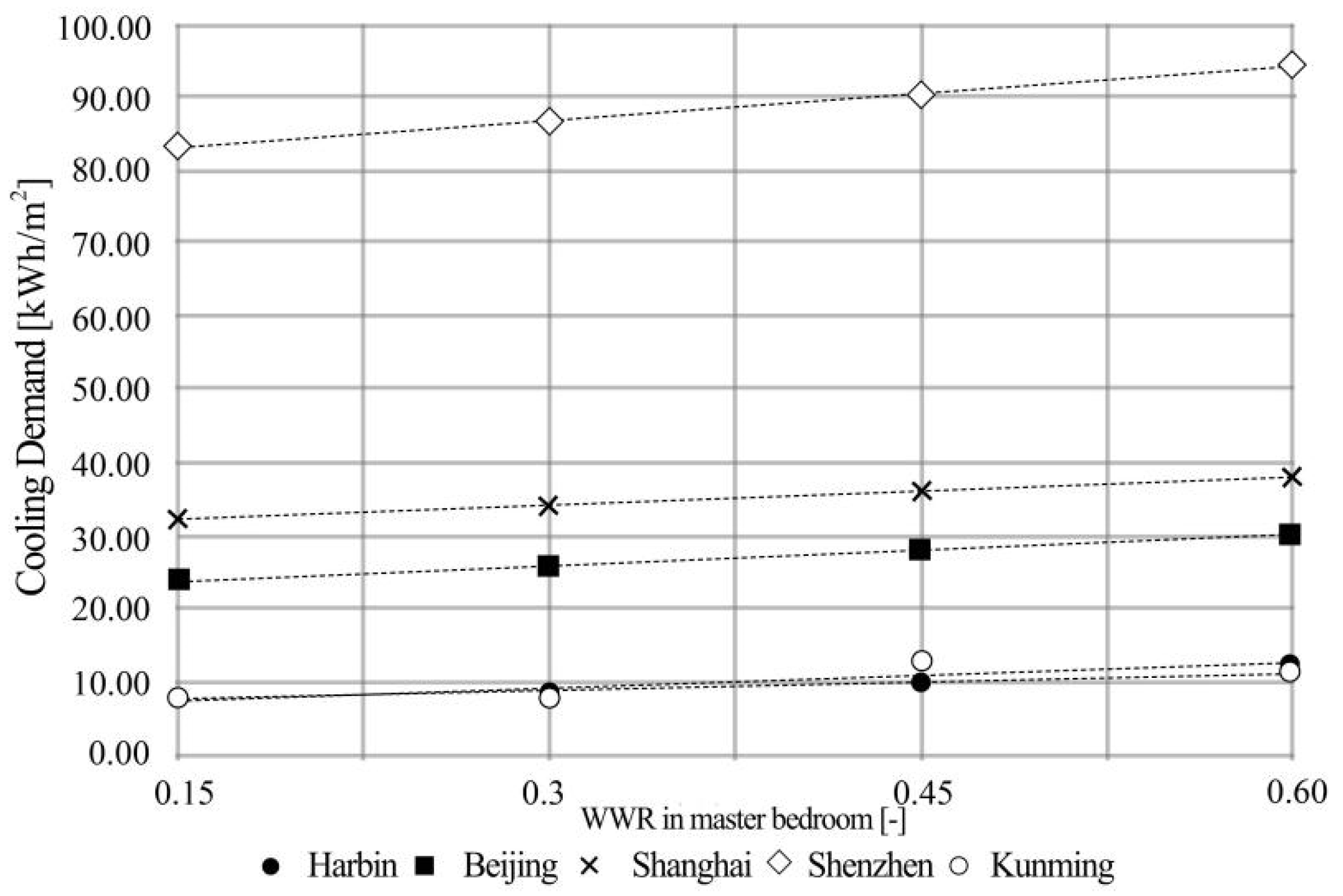
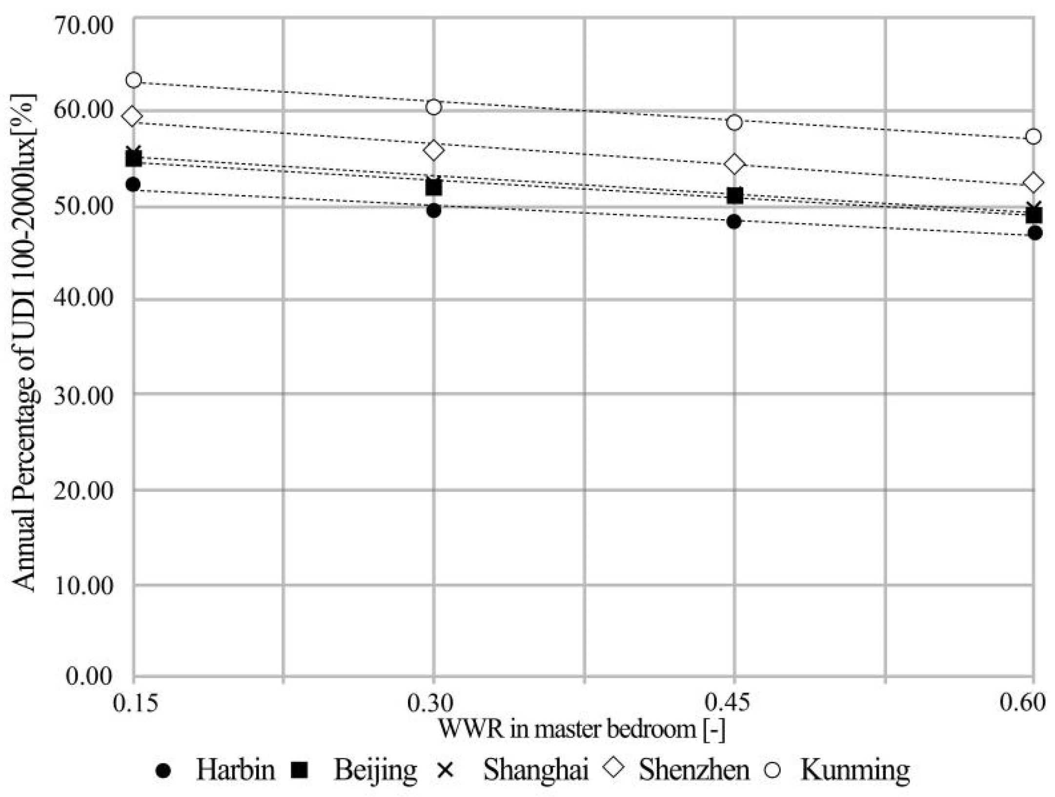
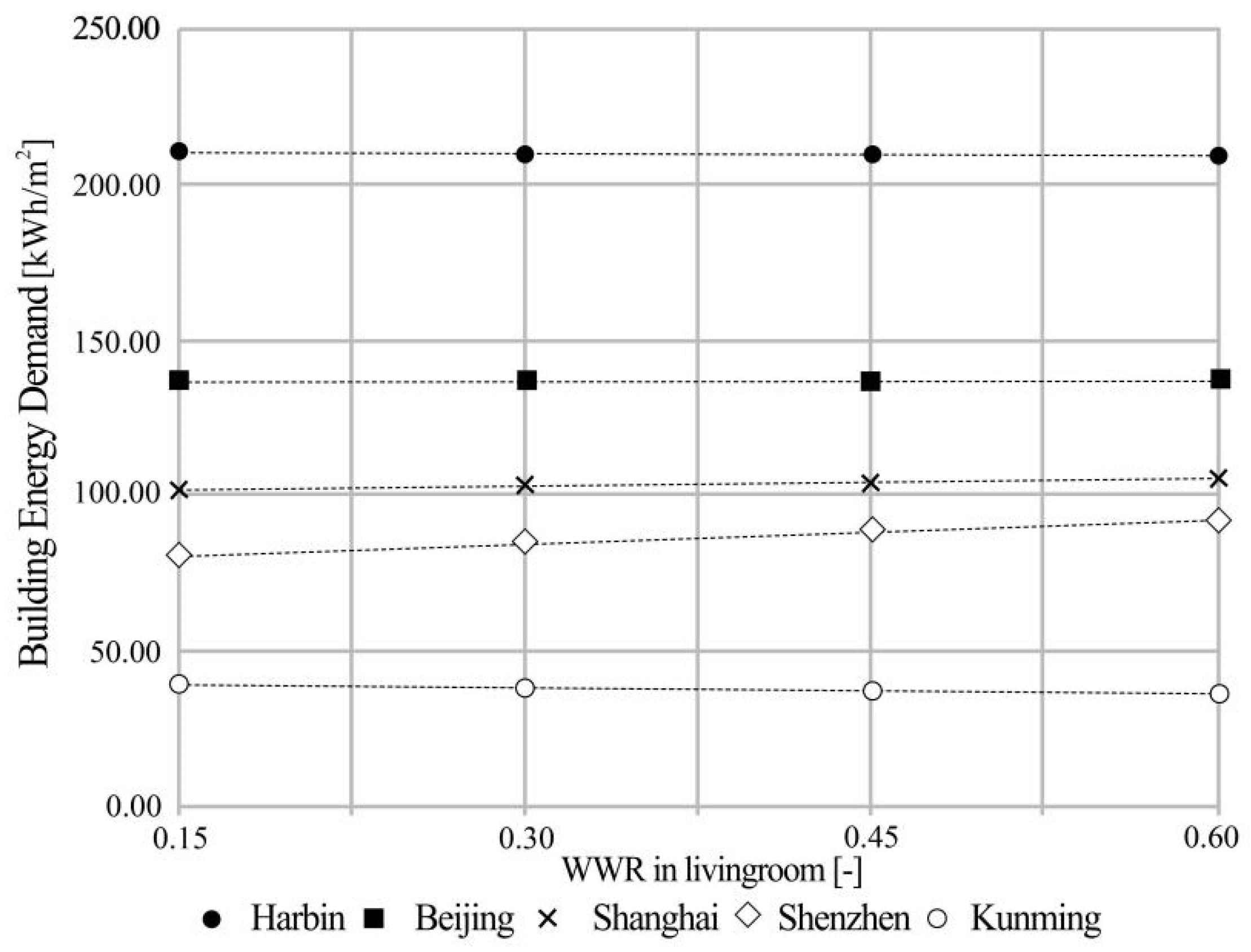
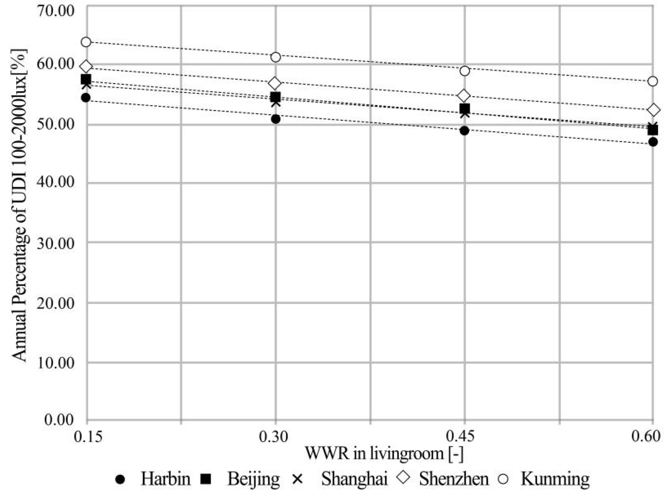
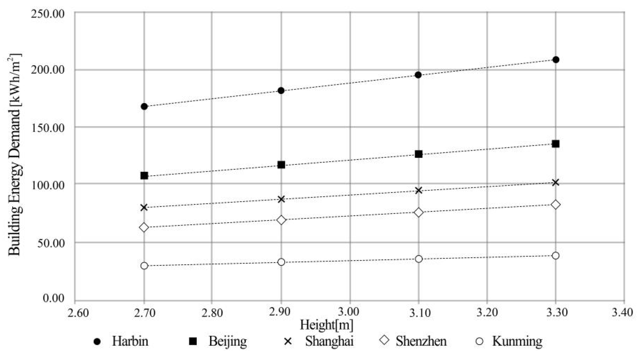
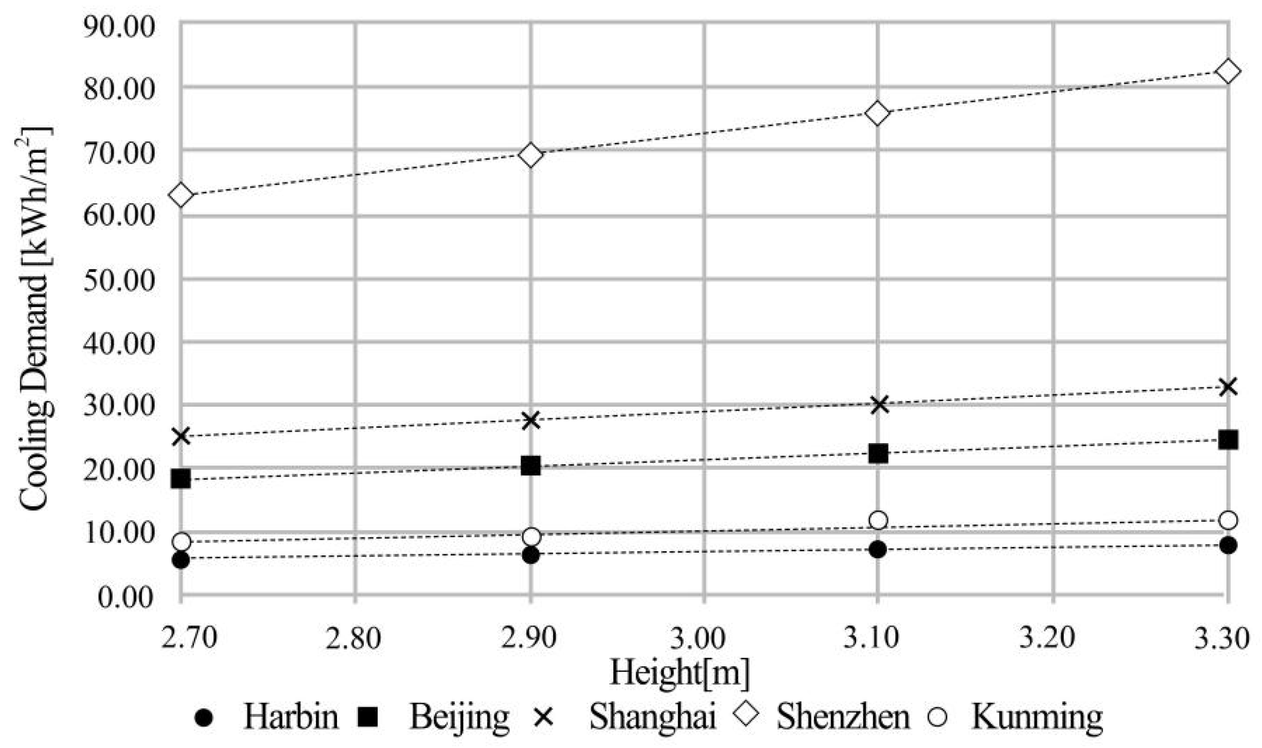
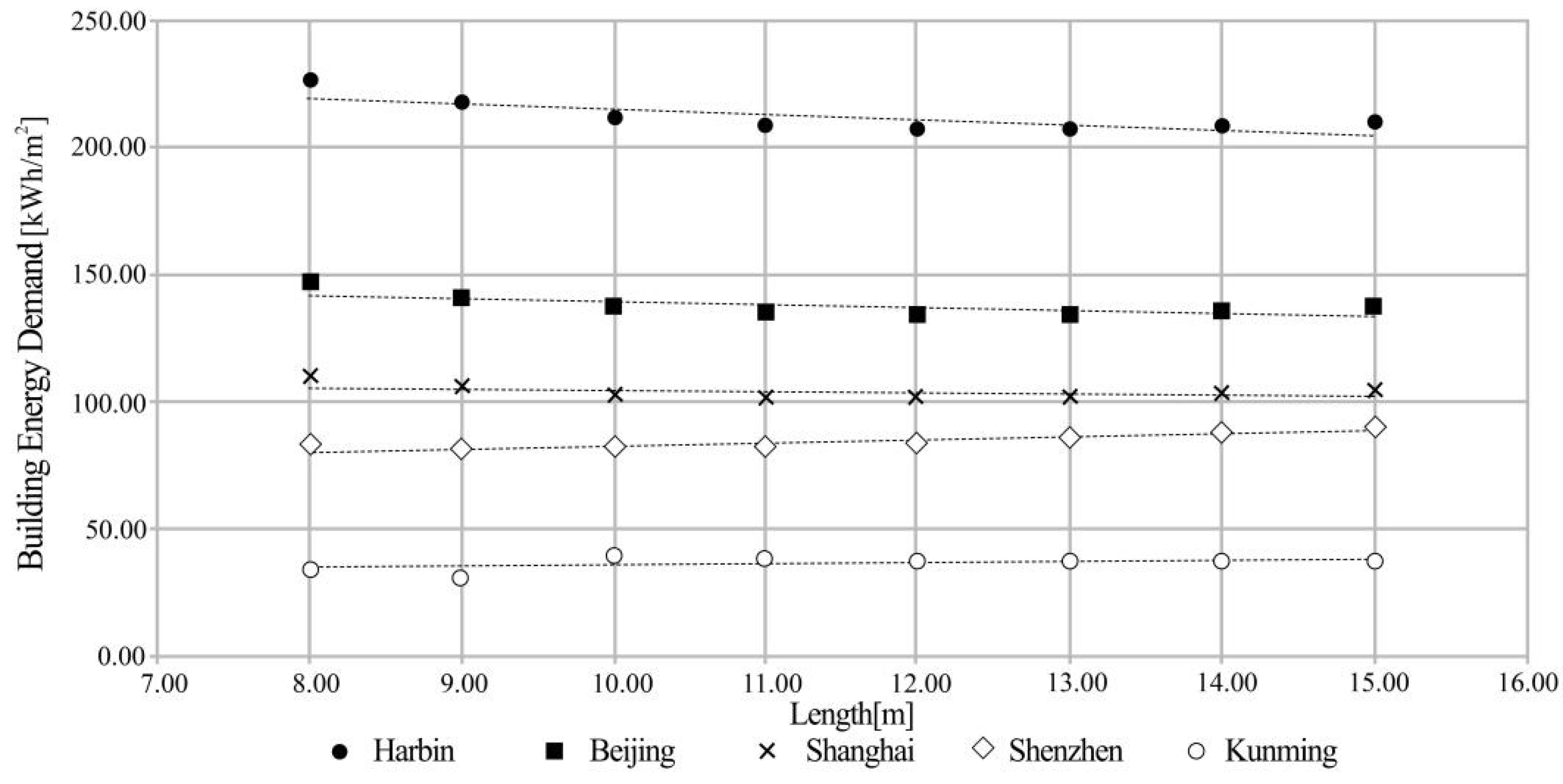
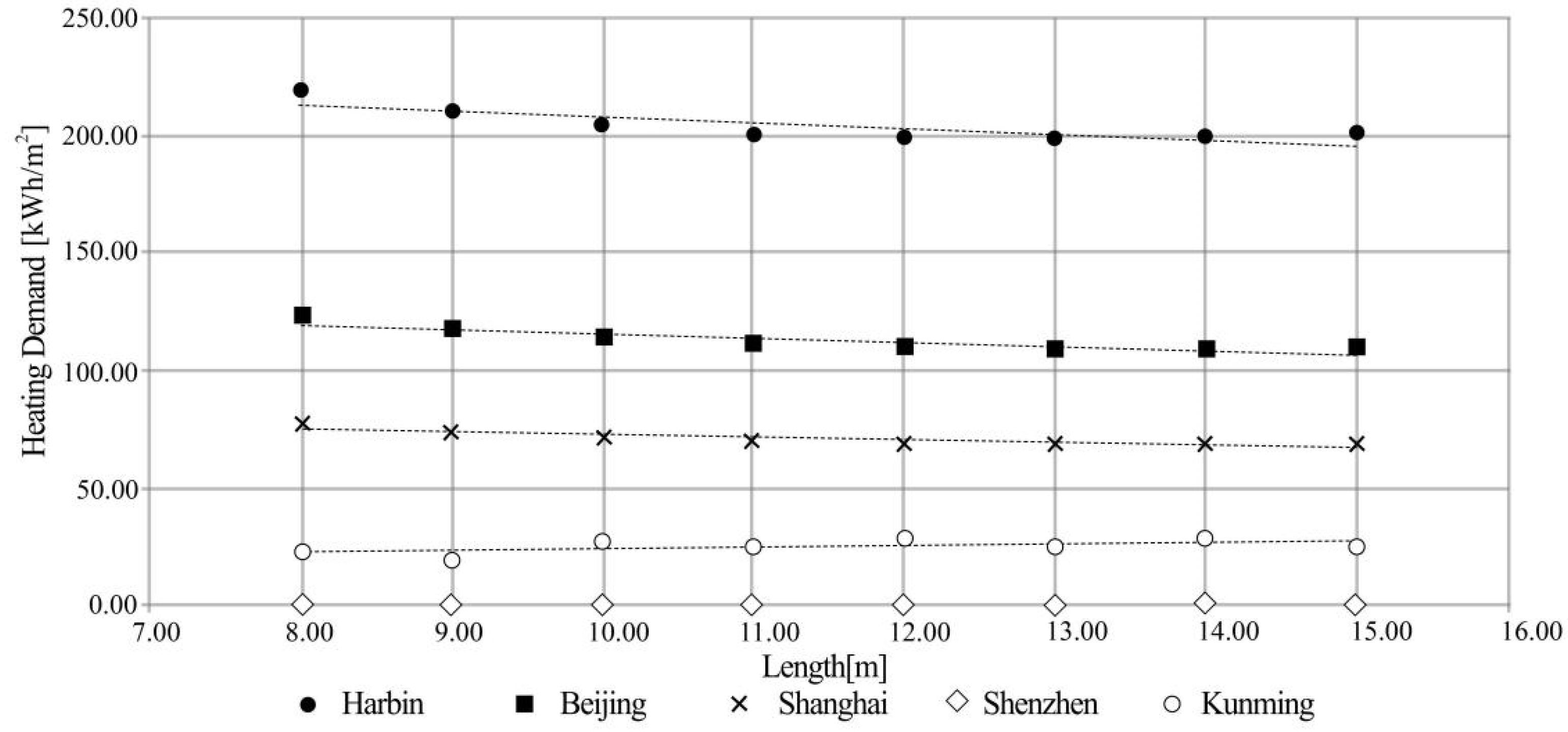
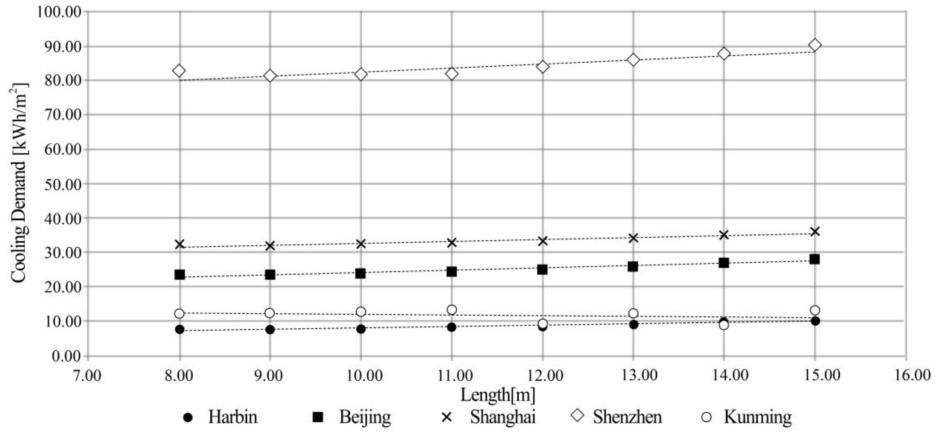
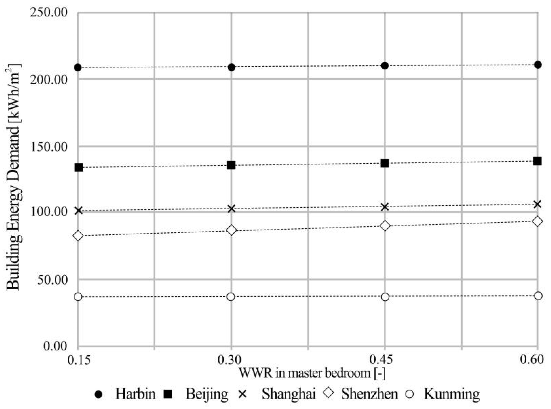
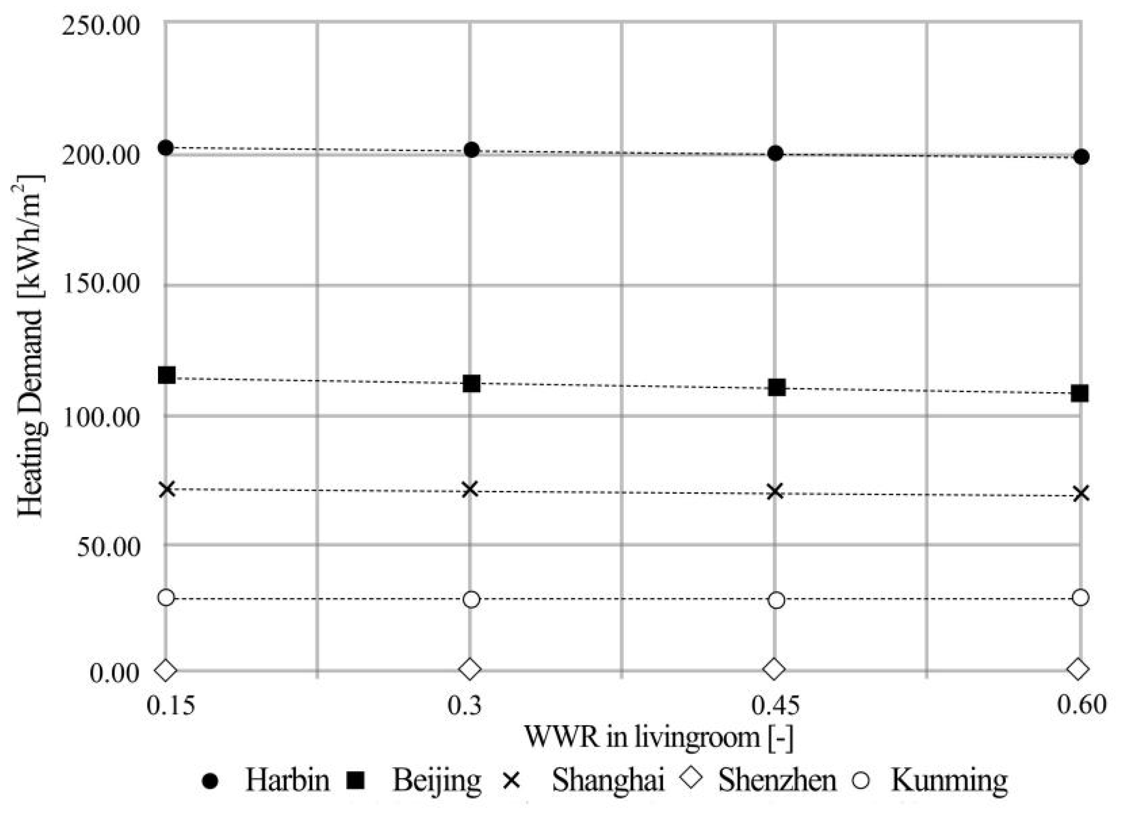
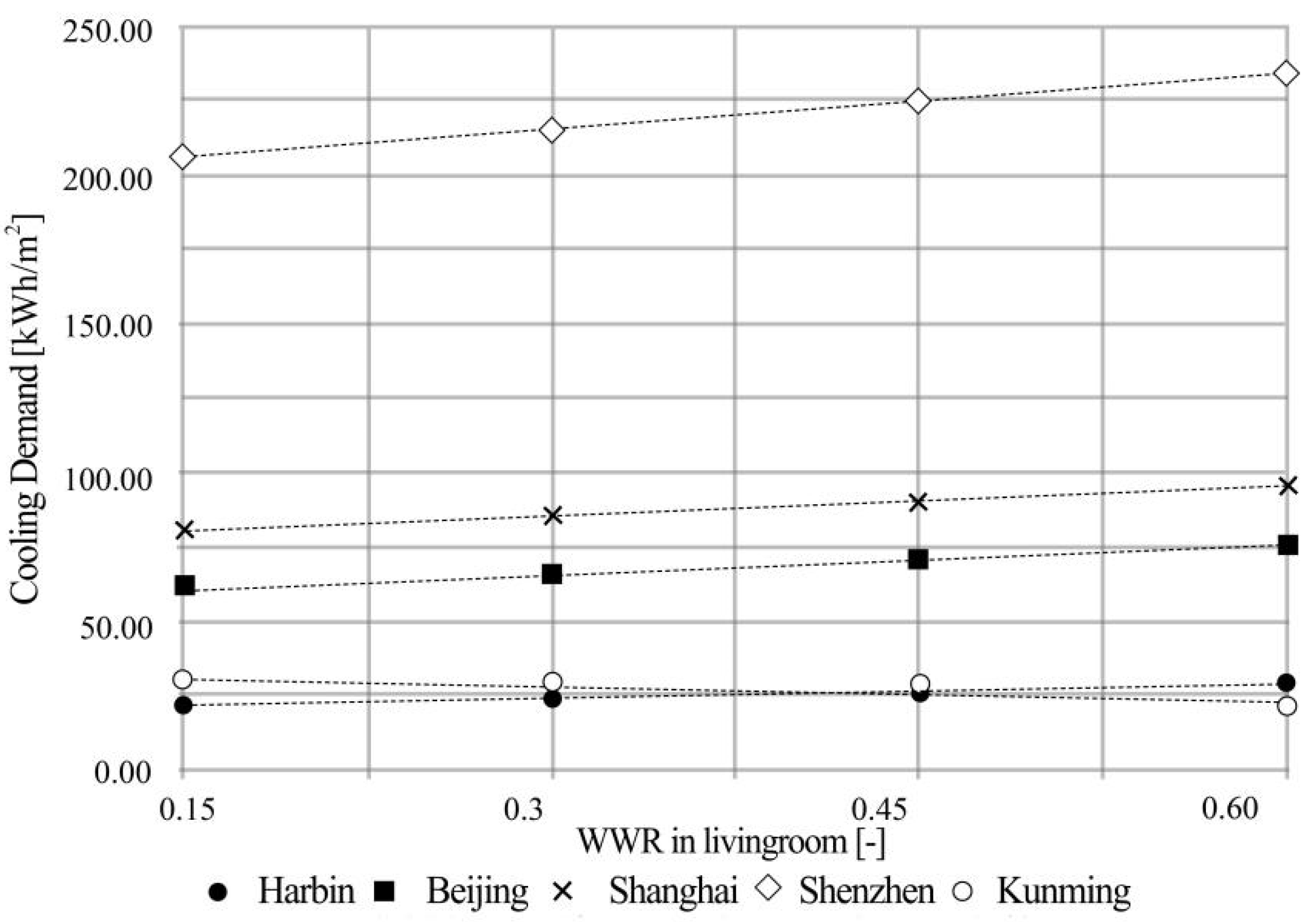
4.3. Sensitivity Analysis of Design Parameters of Residential Interior Space
5. Discussion of Optimization Results
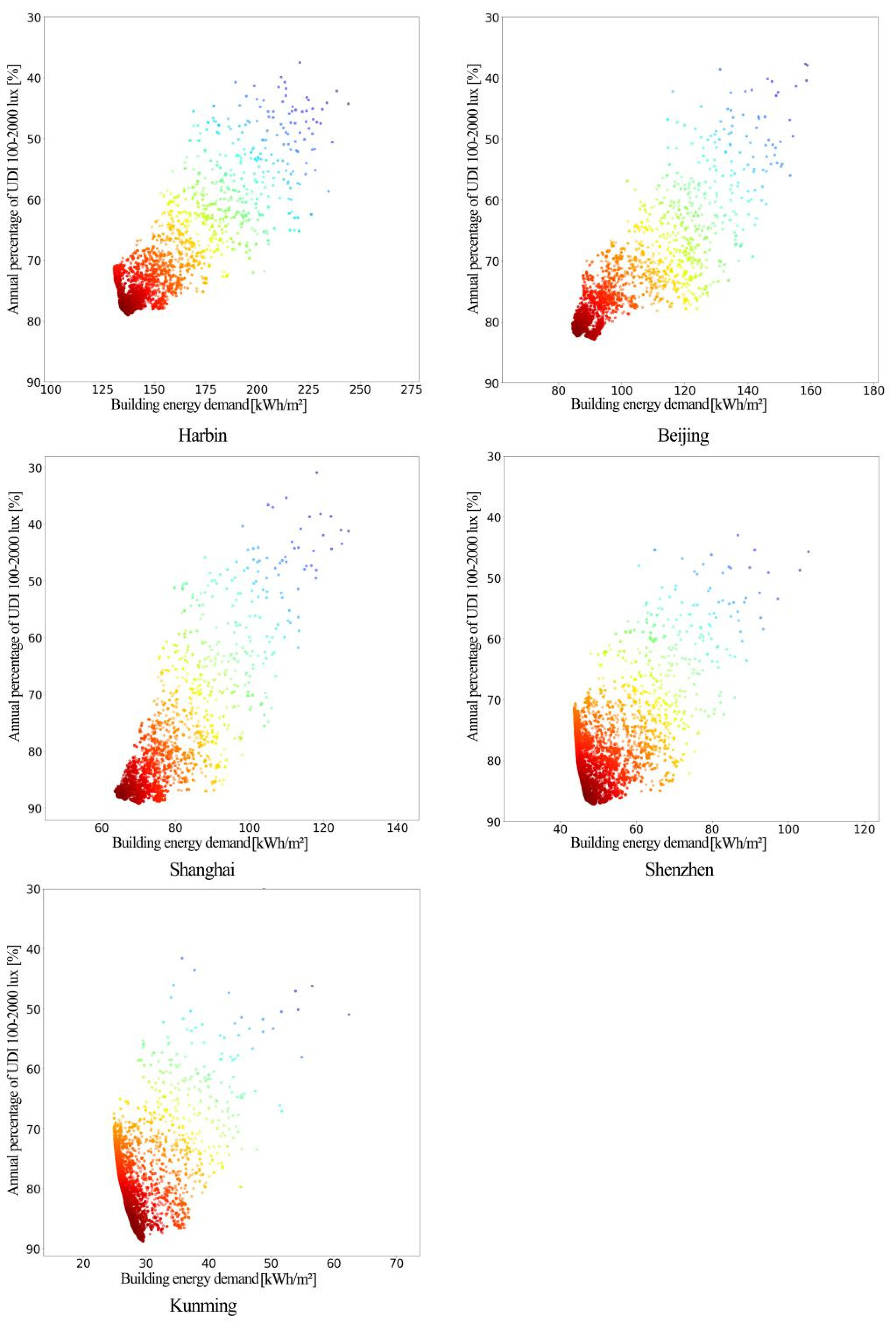
5.1. Optimization Results of Residential Interior Design in Typical Cities
5.2. Comparison of Optimization Results with Reference Model
6. Conclusions
Author Contributions
Funding
Informed Consent Statement
Data Availability Statement
Acknowledgments
Conflicts of Interest
Appendix A


| Classification | Code | Description | Harbin (Severe Cold Area I) | |||||||
|---|---|---|---|---|---|---|---|---|---|---|
| H | C | BED | UDI | |||||||
| C* | S* | C* | S* | C* | S* | C* | S* | |||
| Spatial morphological parameters | A1 | Floor height | 0.891 | 0.00 | 0.397 | 0.00 | 0.898 | 0.00 | 0.237 | 0.00 |
| A2 | Total width | −0.127 | 0.00 | 0.523 | 0.00 | −0.062 | 0.00 | −0.579 | 0.00 | |
| A3 | Total depth | 0.127 | 0.00 | 0.523 | 0.00 | 0.062 | 0.00 | 0.579 | 0.00 | |
| A4 | Master bedroom width | 0.127 | 0.00 | 0.523 | 0.00 | 0.062 | 0.00 | 0.579 | 0.00 | |
| A5 | Master bedroom depth | −0.031 | 0.00 | −0.467 | 0.00 | −0.086 | 0.00 | 0.563 | 0.00 | |
| A6 | Middle bedroom width | −0.127 | 0.00 | 0.523 | 0.00 | −0.062 | 0.00 | −0.579 | 0.00 | |
| A7 | Middle bedroom depth | −0.129 | 0.00 | −0.258 | 0.00 | −0.155 | 0.00 | 0.148 | 0.00 | |
| A8 | North bedroom width | −0.127 | 0.00 | 0.523 | 0.00 | −0.062 | 0.00 | 0.579 | 0.00 | |
| A9 | North bedroom depth | 0.350 | 0.00 | −0.288 | 0.00 | 0.307 | 0.00 | 0.387 | 0.00 | |
| A10 | Kitchen width | 0.049 | 0.00 | 0.316 | 0.00 | 0.085 | 0.00 | −0.344 | 0.00 | |
| A11 | Kitchen depth | 0.350 | 0.00 | −0.288 | 0.00 | 0.307 | 0.00 | 0.387 | 0.00 | |
| Window parameters | B1 | Window-to-wall ratio in north bedroom | 0.065 | 0.00 | 0.177 | 0.00 | 0.084 | 0.00 | −0.124 | 0.00 |
| B2 | Window-to-wall ratio in middle bedroom | 0.028 | 0.00 | 0.288 | 0.00 | 0.061 | 0.00 | −0.159 | 0.00 | |
| B3 | Window-to-wall ratio in master bedroom | −0.036 | 0.00 | 0.437 | 0.00 | 0.018 | 0.00 | −0.292 | 0.00 | |
| B4 | Window-to-wall ratio in living room | −0.054 | 0.00 | 0.409 | 0.00 | −0.003 | 0.00 | −0.405 | 0.00 | |
| B5 | Window-to-wall ratio in kitchen | 0.044 | 0.00 | 0.147 | 0.00 | 0.060 | 0.00 | −0.102 | 0.00 | |
| B6 | Window-to-wall ratio in dining room | 0.034 | 0.00 | 0.074 | 0.00 | 0.042 | 0.00 | −0.070 | 0.00 | |
| Classification | Code | Description | Beijing (Cold Regions II) | |||||||
|---|---|---|---|---|---|---|---|---|---|---|
| H | C | BED | UDI | |||||||
| C* | S* | C* | S* | C* | S* | C* | S* | |||
| Spatial morphological parameters | A1 | Floor height | 0.865 | 0.00 | 0.522 | 0.00 | 0.894 | 0.00 | −0.257 | 0.00 |
| A2 | Total width | −0.196 | 0.00 | 0.472 | 0.00 | 0.001 | 0.00 | −0.588 | 0.00 | |
| A3 | Total depth | 0.196 | 0.00 | −0.472 | 0.00 | −0.001 | 0.00 | 0.588 | 0.00 | |
| A4 | Master bedroom width | −0.196 | 0.00 | 0.472 | 0.00 | 0.001 | 0.00 | −0.588 | 0.00 | |
| A5 | Master bedroom depth | 0.024 | 0.00 | −0.439 | 0.00 | −0.140 | 0.00 | 0.502 | 0.00 | |
| A6 | Middle bedroom width | −0.196 | 0.00 | 0.472 | 0.00 | 0.001 | 0.00 | −0.588 | 0.00 | |
| A7 | Middle bedroom depth | −0.094 | 0.00 | −0.263 | 0.00 | −0.175 | 0.00 | 0.087 | 0.00 | |
| A8 | North bedroom width | −0.196 | 0.00 | 0.472 | 0.00 | 0.001 | 0.00 | −0.588 | 0.00 | |
| A9 | North bedroom depth | 0.397 | 0.00 | −0.221 | 0.00 | 0.263 | 0.00 | 0.510 | 0.00 | |
| A10 | Kitchen width | 0.002 | 0.00 | 0.293 | 0.00 | 0.108 | 0.00 | −0.349 | 0.00 | |
| A11 | Kitchen depth | 0.397 | 0.00 | −0.221 | 0.00 | 0.263 | 0.00 | 0.510 | 0.00 | |
| Window parameters | B1 | Window-to-wall ratio in north bedroom | 0.055 | 0.00 | 0.188 | 0.00 | 0.118 | 0.00 | −0.168 | 0.00 |
| B2 | Window-to-wall ratio in middle bedroom | 0.009 | 0.00 | 0.264 | 0.00 | 0.103 | 0.00 | −0.172 | 0.00 | |
| B3 | Window-to-wall ratio in master bedroom | −0.075 | 0.00 | 0.389 | 0.00 | 0.078 | 0.00 | −0.292 | 0.00 | |
| B4 | Window-to-wall ratio in living room | −0.157 | 0.00 | 0.397 | 0.00 | 0.012 | 0.00 | −0.358 | 0.00 | |
| B5 | Window-to-wall ratio in kitchen | 0.028 | 0.00 | 0.146 | 0.00 | 0.079 | 0.00 | −0.132 | 0.00 | |
| B6 | Window-to-wall ratio in dining room | 0.036 | 0.00 | 0.084 | 0.00 | 0.063 | 0.00 | −0.103 | 0.00 | |
| Classification | Code | Description | Shanghai (Hot Summer and Cold Winter Area III) | |||||||
|---|---|---|---|---|---|---|---|---|---|---|
| H | C | BED | UDI | |||||||
| C* | S* | C* | S* | C* | S* | C* | S* | |||
| Spatial morphological parameters | A1 | Floor height | 0.879 | 0.00 | 0.645 | 0.00 | 0.894 | 0.00 | −0.21 | 0.00 |
| A2 | Total width | −0.172 | 0.00 | 0.396 | 0.00 | 0.078 | 0.00 | −0.599 | 0.00 | |
| A3 | Total depth | 0.172 | 0.00 | −0.396 | 0.00 | −0.078 | 0.00 | 0.599 | 0.00 | |
| A4 | Master bedroom width | −0.172 | 0.00 | 0.396 | 0.00 | 0.078 | 0.00 | 0.599 | 0.00 | |
| A5 | Master bedroom depth | 0.008 | 0.00 | −0.388 | 0.00 | −0.188 | 0.00 | 0.455 | 0.00 | |
| A6 | Middle bedroom width | −0.172 | 0.00 | 0.396 | 0.00 | 0.078 | 0.00 | −0.599 | 0.00 | |
| A7 | Middle bedroom depth | −0.118 | 0.00 | −0.242 | 0.00 | −0.196 | 0.00 | 0.274 | 0.00 | |
| A8 | North bedroom width | −0.172 | 0.00 | 0.396 | 0.00 | 0.078 | 0.00 | −0.599 | 0.00 | |
| A9 | North bedroom depth | 0.387 | 0.00 | −0.148 | 0.00 | 0.190 | 0.00 | 0.405 | 0.00 | |
| A10 | Kitchen width | 0.029 | 0.00 | 0.256 | 0.00 | 0.146 | 0.00 | −0.338 | 0.00 | |
| A11 | Kitchen depth | 0.387 | 0.00 | −0.148 | 0.00 | 0.190 | 0.00 | 0.405 | 0.00 | |
| Window parameters | B1 | Window-to-wall ratio in north bedroom | 0.035 | 0.00 | 0.198 | 0.00 | 0.123 | 0.00 | −0.063 | 0.00 |
| B2 | Window-to-wall ratio in middle bedroom | 0.012 | 0.00 | 0.244 | 0.00 | 0.130 | 0.00 | −0.107 | 0.00 | |
| B3 | Window-to-wall ratio in master bedroom | −0.061 | 0.00 | 0.330 | 0.00 | 0.125 | 0.00 | −0.331 | 0.00 | |
| B4 | Window-to-wall ratio in living room | 0.357 | 0.00 | −0.113 | 0.00 | 0.102 | 0.00 | −0.435 | 0.00 | |
| B5 | Window-to-wall ratio in kitchen | 0.006 | 0.00 | 0.155 | 0.00 | 0.083 | 0.00 | −0.006 | 0.00 | |
| B6 | Window-to-wall ratio in dining room | 0.025 | 0.00 | 0.086 | 0.00 | 0.062 | 0.00 | 0.026 | 0.00 | |
| Classification | Code | Description | Shenzhen (Hot Summer and Warm Winter Area IV) | |||||||
|---|---|---|---|---|---|---|---|---|---|---|
| H | C | BED | UDI | |||||||
| C* | S* | C* | S* | C* | S* | C* | S* | |||
| Spatial morphological parameters | A1 | Floor height | 0.00 | 0.00 | 0.733 | 0.00 | 0.733 | 0.00 | −0.239 | 0.00 |
| A2 | Total width | 0.00 | 0.00 | 0.350 | 0.00 | 0.350 | 0.00 | −0.589 | 0.00 | |
| A3 | Total depth | 0.00 | 0.00 | −0.350 | 0.00 | −0.350 | 0.00 | 0.589 | 0.00 | |
| A4 | Master bedroom width | 0.00 | 0.00 | 0.350 | 0.00 | 0.350 | 0.00 | −0.589 | 0.00 | |
| A5 | Master bedroom depth | 0.00 | 0.00 | −0.369 | 0.00 | −0.369 | 0.00 | 0.429 | 0.00 | |
| A6 | Middle bedroom width | 0.00 | 0.00 | 0.350 | 0.00 | 0.350 | 0.00 | −0.589 | 0.00 | |
| A7 | Middle bedroom depth | 0.00 | 0.00 | −0.253 | 0.00 | −0.253 | 0.00 | 0.023 | 0.00 | |
| A8 | North bedroom width | 0.00 | 0.00 | 0.350 | 0.00 | 0.350 | 0.00 | −0.589 | 0.00 | |
| A9 | North bedroom depth | 0.00 | 0.00 | −0.077 | 0.00 | −0.077 | 0.00 | 0.633 | 0.00 | |
| A10 | Kitchen width | 0.00 | 0.00 | 0.244 | 0.00 | 0.244 | 0.00 | −0.347 | 0.00 | |
| A11 | Kitchen depth | 0.00 | 0.00 | −0.077 | 0.00 | −0.077 | 0.00 | 0.633 | 0.00 | |
| Window parameters | B1 | Window-to-wall ratio in north bedroom | 0.00 | 0.00 | 0.181 | 0.00 | 0.181 | 0.00 | −0.191 | 0.00 |
| B2 | Window-to-wall ratio in middle bedroom | 0.00 | 0.00 | 0.186 | 0.00 | 0.186 | 0.00 | −0.161 | 0.00 | |
| B3 | Window-to-wall ratio in master bedroom | 0.00 | 0.00 | 0.282 | 0.00 | 0.282 | 0.00 | −0.236 | 0.00 | |
| B4 | Window-to-wall ratio in living room | 0.00 | 0.00 | 0.308 | 0.00 | 0.308 | 0.00 | −0.271 | 0.00 | |
| B5 | Window-to-wall ratio in kitchen | 0.00 | 0.00 | 0.132 | 0.00 | 0.132 | 0.00 | −0.165 | 0.00 | |
| B6 | Window-to-wall ratio in dining room | 0.97 | 0.97 | 0.097 | 0.00 | 0.097 | 0.00 | −0.126 | 0.00 | |
| Classification | Code | Description | Kunming (Temperate Region V) | |||||||
|---|---|---|---|---|---|---|---|---|---|---|
| H | C | BED | UDI | |||||||
| C* | S* | C* | S* | C* | S* | C* | S* | |||
| Spatial morphological parameters | A1 | Floor height | 0.808 | 0.00 | 0.278 | 0.00 | 0.838 | 0.00 | −0.238 | 0.00 |
| A2 | Total width | −0.236 | 0.00 | 0.289 | 0.00 | −0.182 | 0.00 | −0.599 | 0.00 | |
| A3 | Total depth | 0.236 | 0.00 | −0.289 | 0.00 | 0.182 | 0.00 | 0.599 | 0.00 | |
| A4 | Master bedroom width | −0.236 | 0.00 | 0.289 | 0.00 | −0.182 | 0.00 | −0.599 | 0.00 | |
| A5 | Master bedroom depth | 0.044 | 0.00 | −0.286 | 0.00 | −0.007 | 0.00 | 0.489 | 0.00 | |
| A6 | Middle bedroom width | −0.236 | 0.00 | 0.289 | 0.00 | −0.182 | 0.00 | −0.599 | 0.00 | |
| A7 | Middle bedroom depth | −0.097 | 0.00 | −0.036 | 0.00 | −0.101 | 0.00 | 0.054 | 0.00 | |
| A8 | North bedroom width | −0.236 | 0.00 | 0.289 | 0.00 | −0.182 | 0.00 | −0.599 | 0.00 | |
| A9 | North bedroom depth | 0.449 | 0.00 | −0.209 | 0.00 | 0.406 | 0.00 | 0.568 | 0.00 | |
| A10 | Kitchen width | −0.012 | 0.00 | 0.179 | 0.00 | 0.020 | 0.00 | −0.362 | 0.00 | |
| A11 | Kitchen depth | 0.449 | 0.00 | −0.209 | 0.00 | 0.406 | 0.00 | 0.568 | 0.00 | |
| Window parameters | B1 | Window-to-wall ratio in north bedroom | 0.029 | 0.00 | 0.137 | 0.00 | 0.052 | 0.00 | −0.169 | 0.00 |
| B2 | Window-to-wall ratio in middle bedroom | −0.023 | 0.00 | 0.601 | 0.00 | 0.069 | 0.00 | −0.161 | 0.00 | |
| B3 | Window-to-wall ratio in master bedroom | −0.101 | 0.00 | 0.457 | 0.00 | −0.023 | 0.00 | −0.257 | 0.00 | |
| B4 | Window-to-wall ratio in living room | −0.248 | 0.00 | 0.162 | 0.00 | −0.215 | 0.00 | −0.278 | 0.00 | |
| B5 | Window-to-wall ratio in kitchen | 0.003 | 0.00 | 0.125 | 0.00 | 0.025 | 0.00 | −0.137 | 0.00 | |
| B6 | Window-to-wall ratio in dining room | 0.018 | 0.00 | 0.032 | 0.00 | 0.024 | 0.00 | −0.100 | 0.00 | |
References
- U.S. Energy Information Administration. Annual Energy Outlook 2014; US Department of Energy: Washington, DC, USA, 2014; Volume 0383, pp. 1–269.
- Guo, S.; Yan, D.; Hu, S.; Zhang, Y. Modelling building energy consumption in China under different future scenarios. Energy 2021, 214, 119063. [Google Scholar] [CrossRef]
- Kylili, A.; Fokaides, P.A.; Jimenez, P.A.L. Key Performance Indicators (KPIs) approach in buildings renovation for the sustainability of the built environment: A review. Renew. Sustain. Energy Rev. 2016, 56, 906–915. [Google Scholar] [CrossRef]
- Xu, W.; Liu, Z.; Chen, X.; Zhang, S.C. Thoughts of development of Chinese nearly zero energy buildings. Build. Sci. 2016, 32, 1–5. [Google Scholar]
- UN General Assembly. Transforming Our World: The 2030 Agenda for Sustainable Development; A/RES/70/1; UN General Assembly: New York, NY, USA, 2015. [Google Scholar]
- D′Agostino, D. Assessment of the progress towards the establishment of definitions of Nearly Zero Energy Buildings (nZEBs) in European Member States. J. Build. Eng. 2015, 1, 20–32. [Google Scholar] [CrossRef]
- Teitelbaum, E.; Jayathissa, P.; Miller, C. Forrest Meggers, Design with Comfort: Expanding the psychrometric chart with radiation and convection dimensions. Energy Build. 2020, 209, 109591. [Google Scholar] [CrossRef]
- Olgyay, V. Design with Climate, Bioclimatic Approach to Architectural Regionalism; Princeton University Press: Princeton, NJ, USA, 1963; p. 125. [Google Scholar]
- Givoni, B. Man, Climate and Architecture; Applied Science Publisher: London, UK, 1969. [Google Scholar]
- Alsousi, M. User Response to Energy Conservation and Thermal Comfort of High-Rise Residential Buildings in Hot Humid Region with Referring to Gaza. Ph.D. Thesis, University of Nottingham, Nottingham, UK, 2005. [Google Scholar]
- Ghisi, E.; Massignani, R.F. Thermal performance of bedrooms in a multi-storey residential building in southern Brazil. Build. Environ. 2007, 42, 730–742. [Google Scholar] [CrossRef]
- Schnieders, J.; Feist, W.; Rongen, L. Passive Houses for different climate zones. Energy Build. 2015, 105, 71–87. [Google Scholar] [CrossRef]
- Martinelli, L.; Matzarakis, A. Influence of height/width proportions on the thermal comfort of courtyard typology for Italian climate zones. Sustain. Cities Soc. 2017, 29, 97–106. [Google Scholar] [CrossRef]
- Harkouss, F.; Fardoun, F.; Biwole, P. Passive design optimization of low energy buildings in different climates. Energy 2018, 165, 591–613. [Google Scholar] [CrossRef]
- Harkouss, F. Optimal Design of Net Zero Energy Buildings under Different Climates. Ph.D. Thesis, Université Côte d’Azur, Provence, France, Université Libanaise, Beirut, Lebanon, 2018. [Google Scholar]
- Ascione, F.; Bianco, N.; Mauro, G.M.; Napolitano, D.F. Building envelope design: Multi-objective optimization to minimize energy consumption, global cost and thermal discomfort. Application to different Italian climatic zones. Energy 2019, 174, 359–374. [Google Scholar] [CrossRef]
- Coma, J.; Maldonado, J.M.; de Gracia, A.; Gimbernat, T.; Botargues, T.; Cabeza, L.F. Comparative Analysis of Energy Demand and CO2 Emissions on Different Typologies of Residential Buildings in Europe. Energies 2019, 12, 2436. [Google Scholar] [CrossRef] [Green Version]
- Ciancio, V.; Salata, F.; Falasca, S.; Curci, G.; Golasi, I.; de Wilde, P. Energy demands of buildings in the framework of climate change: An investigation across Europe. Sustain. Cities Soc. 2020, 60, 102213. [Google Scholar] [CrossRef]
- Ciardiello, A.; Rosso, F.; Dell’Olmo, J.; Ciancio, V.; Ferrero, M.; Salata, F. Multi-objective approach to the optimization of shape and envelope in building energy design. Appl. Energy 2020, 280, 115984. [Google Scholar] [CrossRef]
- Kheiri, F. A review on optimization methods applied in energy-efficient building geometry and envelope design. Renew. Sustain. Energy Rev. 2018, 92, 897–920. [Google Scholar] [CrossRef]
- Shin, Y.; Cho, H.; Kang, K.-I. Simulation model incorporating genetic algorithms for optimal temporary hoist planning in high-rise building construction. Autom. Constr. 2011, 20, 550–558. [Google Scholar] [CrossRef]
- Holland, J.H. Adaptation in Natural and Artificial Systems: An Introductory Analysis with Applications to Biology, Control, and Artificial Intelligence; MIT Press: Cambridge, MA, USA, 1992. [Google Scholar]
- EPBD: Directive 2010/31/EU of the European Parliament and of the Council of 19 May 2010 on the Energy Performance of Buildings (Recast)[EB/OL]. Available online: http://ec.europa.eu/energy/efficiency/buildings/buildings_en.htm (accessed on 18 June 2010).
- Ferrara, M.; Fabrizio, E.; Virgone, J.; Filippi, M. A simulation-based optimization method for cost-optimal analysis of nearly Zero Energy Buildings. Energy Build. 2014, 84, 442–457. [Google Scholar] [CrossRef]
- Thalfeldt, M.; Pikas, E.; Kurnitski, J.; Voll, H. Facade design principles for nearly zero energy buildings in a cold climate. Energy Build. 2013, 67, 309–321. [Google Scholar] [CrossRef]
- Chantrelle, F.P.; Lahmidi, H.; Keilholz, W.; El Mankibi, M.; Michel, P. Development of a multicriteria tool for optimizing the renovation of buildings. Appl. Energy 2011, 88, 1386–1394. [Google Scholar] [CrossRef]
- Karaguzel, O.T.; Zhang, R.; Lam, K.P. Coupling of whole-building energy simulation and multi-dimensional numerical optimization for minimizing the life cycle costs of office buildings. Build. Simul. 2014, 7, 111–121. [Google Scholar] [CrossRef]
- Prada, A.; Pernigotto, G.; Cappelletti, F.; Gasparella, A.; Jan, L.M. HENSEN. Robustness of multi-objective optimization of building refurbishment to suboptimal weather data. In Proceedings of the International High Performance Building Conference, Purdue, IN, USA, 14–17 July 2014. [Google Scholar]
- Pernigotto, G.; Prada, A.; Cappelletti, F.; Gasparella, A. Impact of Reference Years on the Outcome of Multi-Objective Optimization for Building Energy Refurbishment. Energies 2017, 10, 1925. [Google Scholar] [CrossRef] [Green Version]
- Ascione, F.; Bianco, N.; De Stasio, C.; Mauro, G.M.; Vanoli, G.P. Multi-stage and multi-objective optimization for energy retrofitting a developed hospital reference building: A new approach to assess cost-optimality. Appl. Energy 2016, 174, 37–68. [Google Scholar] [CrossRef]
- Asl, M.R.; Zarrinmehr, S.; Bergin, M.; Yan, W. BPOpt: A framework for BIM-based performance optimization. Energy Build. 2015, 108, 401–412. [Google Scholar]
- Echenagucia, T.M.; Capozzoli, A.; Cascone, Y.; Sassone, M. The early design stage of a building envelope: Multi-objective search through heating, cooling and lighting energy performance analysis. Appl. Energy 2015, 154, 577–591. [Google Scholar] [CrossRef]
- Bre, F.; Silva, A.S.; Ghisi, E.; Fachinotti, V. Residential Building Design Optimisation Using Sensitivity Analysis and Genetic Algorithm. Energy Build. 2016, 133, 853–866. [Google Scholar] [CrossRef]
- Toutou, A. A Parametric Approach for Achieving Optimum Residential Building Performance in Hot Arid Zone. Master’s Thesis, Alexandria University, Alexandria, Egypt, 2018. [Google Scholar]
- Gagnon, R.; Gosselin, L.; Decker, S.A. Performance of a sequential versus holistic building design approach using multi-objective optimization. J. Build. Eng. 2019, 26, 100883. [Google Scholar] [CrossRef]
- Li, Y.; Bonyadi, N.; Papakyriakou, A.; Lee, B. A hierarchical decomposition approach for multi-level building design optimization. J. Build. Eng. 2021, 44, 103272. [Google Scholar] [CrossRef]
- Zhang, T.; Wang, D.; Liu, H.; Liu, Y.; Wu, H. Numerical investigation on building envelope optimization for low-energy buildings in low latitudes of China. Build. Simul. 2020, 13, 257–269. [Google Scholar] [CrossRef]
- Li, Z.; Tian, M.; Zhao, Y.; Zhang, Z.; Ying, Y. Development of an Integrated Performance Design Platform for Residential Buildings Based on Climate Adaptability. Energies 2021, 14, 8223. [Google Scholar] [CrossRef]
- Xu, Y.; Zhang, G.; Yan, C.; Wang, G.; Jiang, Y.; Zhao, K. A two-stage multi-objective optimization method for envelope and energy generation systems of primary and secondary school teaching buildings in China. Build. Environ. 2021, 204, 108142. [Google Scholar] [CrossRef]
- Diamond, R.C.; Ye, Q.; Feng, W.; Yan, T.; Mao, H.; Li, Y.; Guo, Y.; Wang, J. Sustainable Building in China—A Green Leap Forward? Buildings 2013, 3, 639–6582. [Google Scholar] [CrossRef]
- Lush, D.; Butcher, K.; Appleby, P. Environmental Design: CIBSE Guide A; The Chartered Institution of Building Services Engineers: London, UK, 2006. [Google Scholar]
- Ramallo-González, A.P. Modelling, Simulation and Optimisation Methods for Low-Energy Buildings. Ph.D. Thesis, University of Exeter, Stocker, UK, 2013. [Google Scholar]
- Shi, L.; Zhang, Y.; Wang, Z.; Cheng, X.; Yan, H. Luminance parameter thresholds for user visual comfort under daylight conditions from subjective responses and physiological measurements in a gymnasium. Build. Environ. 2021, 205, 108187. [Google Scholar] [CrossRef]
- ASHRAE Handbook Fundamentals; American Society of Heating, Refrigerating and Air-Conditioning Engineers: Atlanta, GA, USA, 2009.
- Pedersen, C.O.; Fisher, D.E.; Liesen, R.J. Development of a heat balance procedure for calculating cooling loads. ASHRAE Trans. 1997, 103, 459–468. [Google Scholar]
- Walton, G.N. Thermal Analysis Research Program Reference Manual; National Bureau of Standards: Gaithersburg, MD, USA, 1983.
- Balali, A.; Valipour, A. Prioritization of passive measures for energy optimization designing of sustainable hospitals and health centres. J. Build. Eng. 2020, 35, 101992. [Google Scholar] [CrossRef]
- Nabil, A.; Mardaljevic, J. Useful daylight illuminances: A replacement for daylight factors. Energy Build. 2006, 38, 905–913. [Google Scholar] [CrossRef]
- Wang, Y.; Li, C.; Jin, X.; Xiang, Y.; Li, X. Multi-objective optimization of rolling schedule for tandem cold strip rolling based on NSGA-II. J. Manuf. Process. 2020, 60, 257–267. [Google Scholar] [CrossRef]
- Gan, Y.; Yang, M.; Sun, F.; Yang, L. A quantitative model and solution of reaction heat for microfluidic chips based on Kriging and NSGA-II. Thermochim. Acta. 2020, 694, 178803. [Google Scholar] [CrossRef]
- Liu, D.; Huang, Q.; Yang, Y.; Liu, D.; Wei, X. Bi-objective algorithm based on NSGA-II framework to optimize reservoirs operation. J. Hydrol. 2020, 585, 124830. [Google Scholar] [CrossRef]
- Delgarm, N.; Sajadi, B.; Delgarm, S.; Kowsary, F. A novel approach for the simulation-based optimization of the buildings energy consumption using NSGA-II: Case study in Iran. Energy Build. 2016, 127, 552–560. [Google Scholar] [CrossRef]
- Zhou, Y.; Cao, S.; Kosonen, R.; Hamdy, M. Multi-objective optimisation of an interactive buildings-vehicles energy sharing network with high energy flexibility using the Pareto archive NSGA-II algorithm. Energy Convers. Manag. 2020, 218, 113017. [Google Scholar] [CrossRef]
- Yusoff, Y.; Ngadiman, M.S.; Zain, A.M. Overview of NSGA-II for Optimizing Machining Process Parameters. Procedia Eng. 2011, 15, 3978–3983. [Google Scholar] [CrossRef] [Green Version]
- Roman, N.D.; Bre, F.; Fachinotti, V.D.; Lamberts, R. Application and characterization of metamodels based on artificial neural networks for building performance simulation: A systematic review. Energy Build. 2020, 217, 109972. [Google Scholar] [CrossRef]
- Buratti, C.; Orestano, F.C.; Palladino, D. Comparison of the Energy Performance of Existing Buildings by Means of Dynamic Simulations and Artificial Neural Networks. Energy Procedia 2016, 101, 176–183. [Google Scholar] [CrossRef]
- Magnier, L.; Haghighat, F. Multiobjective optimization of building design using TRNSYS simulations, genetic algorithm, and Artificial Neural Network. Build. Environ. 2010, 45, 739–746. [Google Scholar] [CrossRef]
- Neto, A.H.; Fiorelli, F.A.S. Comparison between detailed model simulation and artificial neural network for forecasting building energy consumption. Energy Build. 2008, 40, 2169–2176. [Google Scholar] [CrossRef]
- Mukhamet, T.; Kobeyev, S.; Nadeem, A.; Memon, S.A. Ranking PCMs for building façade applications using multi-criteria decision-making tools combined with energy simulation. Energy 2021, 215 Pt B, 119102. [Google Scholar] [CrossRef]


| Authors | Time | Main Work | Reference |
|---|---|---|---|
| V. Olgyay | 1953 | He first proposed the building climate analysis method which recommended architects to use passive means to adjust the building microclimate in architectural design. | [7] |
| V. Olgyay | 1963 | He published “Design with Climate” which proposed to adopt a passive design method to maximize the use of renewable energy such as solar energy and wind energy, as well as reduce building energy consumption. | [8] |
| B. Givoni | 1976 | He improved Olgyay’s bioclimatic chart and proposed architectural bioclimatic design method based on climate environment and distinguished it from Olgyay’s method. Architectural bioclimate design requires that, in the process of architectural design, solve the problems of the architectural environment by making use of natural conditions as much as possible, propose corresponding architectural technical means and control methods, and create a more comfortable and healthier environment that meets the requirements of modern society on the basis of respecting the nature environment. | [9] |
| M. Alsousi et al. | 2005 | They studied the climate responsive design of buildings in Gaza and investigated 12 high-rise residential buildings in terms of thermal comfort and energy consumption. The researchers finally found that most of the building energy consumption in summer is caused by the heat generated by the walls, windows and roof. In addition, the occupants, daily life facilities and air infiltration will also increase the building energy consumption, while the effect of them on the thermal performance and occupants’ comfort are relatively small. | [10] |
| Enedir Ghisi and Ricardo Felipe Massignani | 2007 | They tested the thermal performance of a multi-story residential building in southern Brazil. They recorded the thermal performance of eight bedrooms on two floors and four directions. Different variables are used to examine various factors, such as surface color, window shadow and thermal properties of walls and windows. Finally, it is concluded that the heating transmittance and area of the building envelope have the greatest influence on the maximum temperature, and it needs to be minimized to improve the indoor thermal environment in summer. While heat capacity and thermal time lag have the strongest correlation with the minimum temperature, so they should be maximized to improve the thermal environment comfort in winter. | [11] |
| Jürgen Schnieders et al. | 2015 | They used the same typical analysis model to analyze and compare the design strategies of passive housing, including envelope design, air tightness, operation of cooling coil, heat recovery equipment and supply air temperature, etc., taking Yekaterinburg, Tokyo, Shanghai, Las Vegas, Abu Dhabi and Singapore as examples, to propose the corresponding design guidelines for passive buildings. | [12] |
| Letizia Martinelli and Andreas Matzarakis | 2017 | They selected six Italian cities as representatives, including Aosta, Milan, Campobasso, Florence, Lecce and Catania. Based on the climate data of each city in the past 30 years, the influence of courtyard-type parameters such as the ratio of height to width on the humidity and thermal comfort of the courtyards of various cities in different climate zones is analyzed. | [13] |
| Fatima Harkouss et al. | 2018 | They selected 25 typical cities in different climate regions to simulate and optimize the passive design of residential buildings according to the Kӧppen climate zoning. He compared the performance of residential buildings in different cities by taking the life cycle cost (LCC) and building cooling and heating consumption as objective functions, to obtain the corresponding energy-saving design strategy. | [14,15] |
| Fabrizio Ascione et al. | 2019 | They used MATLAB, EnergyPlus and genetic algorithm to compare the multi-objective optimization of residential buildings in typical cities in different climates in Italy and obtained the envelope design strategy for each climate zone. | [16] |
| Julià Coma et al. | 2019 | Based on the European residential building database compiled by the TABULA/EPISCOPE project, they analyzed and compared the energy-saving strategies of many European countries with building energy consumption and carbon dioxide emissions as indicators. They also evaluated the feasibility of using new energy technologies in different cities in hot, warm and cold climate zones in Europe. | [17] |
| Virgilio Ciancio et al. | 2020 | They discussed the impact of climate warming on residential buildings in 19 different cities in Europe based on the Kӧppen climate zoning. They concluded that the gradual increase of average climate temperature from 2050 to 2080 will lead to the decrease of heating energy consumption of residential buildings, and the increase of cooling energy consumption and carbon dioxide concentration. Moreover, cities in the Mediterranean climate zone are more affected by global heating than inland cities in Europe. This trend can be alleviated by improving the buildings’ energy efficiency. | [18] |
| Authors | Time | Main Work | Reference |
|---|---|---|---|
| Fanny Pernodet Chantrelle et al. | 2011 | They used NSGA-II algorithm (Non-dominated Sorting Genetic Algorithm) and dynamic simulation tool TRNSYS to carry out multi-objective optimization design of building envelope and shading control strategy based on building energy consumption, cost, thermal comfort and environmental protection. | [26] |
| Omer T. Karaguzel et al. | 2014 | They combined the building energy simulation software EnergyPlus and the optimization tool GenOpt to optimize the life cycle cost of a commercial office building. | [27] |
| Alessandro Prada et al. | 2014 | They implemented a comprehensive framework of multi-objective energy optimization in buildings, and used EnergyPlus and NSGA-II algorithm for building environment simulation and multi-objective optimization to search Pareto frontier for building energy-efficiency design. | [28,29] |
| Fabrizio Ascione et al. | 2014 | They combined MATLAB and EnergyPlus to optimize the construction plan of a hospital building with multiple goals. The optimization goals are the primary energy consumption of the building, the initial investment and global cost of the renovation plan. | [30] |
| Mohammad Rahmani Asl et al. | 2015 | They presented an integrated framework for building information modeling (BIM)-based performance optimization, BPOpt. | [31] |
| Tomás Méndez Echenagucia et al. | 2015 | An integrative approach for the early stages of building design is proposed to obtain detailed information on energy-efficient envelope configurations. | [32] |
| Facundo Bre et al. | 2016 | They took daylighting and energy saving as optimization goals, and used sensitivity analysis and genetic algorithms to optimize the design of typical independent houses. | [33] |
| Ahmed Toutou | 2018 | They discussed the potential of parametric algorithms to optimize residential design lighting and thermal performance. | [34] |
| Richard Gagnon et al. | 2019 | Through a case study of a residential building, they compared a sequential versus a holistic design approach based on multi-objective optimization. | [35] |
| Yin Li et al. | 2019 | They proposed a hierarchical decomposition approach that can achieve global optimal solutions. This approach was applied to a multi-objective optimization problem to minimize the carbon emissions and operating costs of buildings. | [36] |
| Tianqi Zhang et al. | 2020 | This research calculated the energy-saving effect of buildings with different shape parameters and the cooling load of thermal performance of different envelope by numerical simulation. In addition, the corresponding energy-saving indexes for cooling load reduction (CLR) are presented. | [37] |
| Zhixing Li et al. | 2021 | They proposed an integrated multi-objective multivariate framework for building performance optimization. Then, a comparison of the performance indicators of low-rise and medium-rise residential buildings under five typical urban climatic conditions are carried out. | [38] |
| Yizhe Xu et al. | 2021 | They proposed a two-stage multi-objective optimization method based on a meta-model to obtain the optimal design scheme for primary and secondary school education buildings, based on daylighting, thermal comfort, energy savings and economy. | [39] |
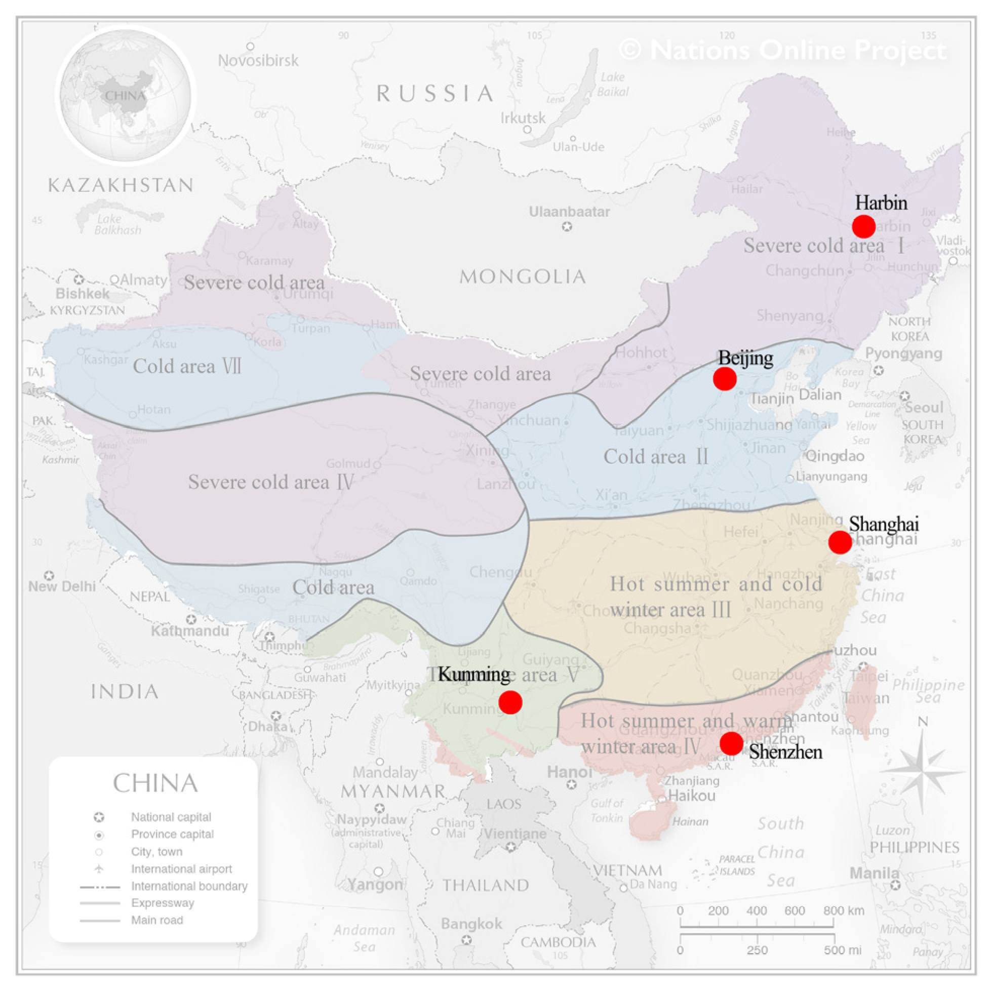
| Climate Zone | Typical City | Heating Degree Day (18 °C) | Heating Period (Day/Month) | Heating Hours per Day |
|---|---|---|---|---|
| Severe cold area I | Harbin | ≥3800 | 20/10 to 15/4 | 24 h |
| Cold region II | Beijing | 2000–3799 | 15/11 to 31/3 | 24 h |
| Hot summer and cold winter area III | Shanghai | 700–1999 | There is no mandatory requirement | – |
| Hot summer and warm winter area IV | Shenzhen | <500 | There is no mandatory requirement (according to the actual demand, heating time is not set in the simulation) | – |
| Temperate region V | Kunming | <2000 | There is no mandatory requirement (but it is set to 15/12 to 1/3 in the simulation according to the actual demand) | – |
| Type | Subcategory | Parameter Category | Unit | Baseline Model |
|---|---|---|---|---|
| Geographical position | Climate | Climate data of Tianjin | – | Climate data of Tianjin |
| Architectural form parameters | Building type | Number of layers | – | 2.00 |
| Net height of each floor | m | 3.30 | ||
| Total height of each floor | m | 3.60 | ||
| Width (s/N direction) | m | 13.5 | ||
| Aspect ratio | – | 2.15 | ||
| Window-to-wall ratio (WWR) | – | 0.35 | ||
| Orientation | deg | 0 | ||
| Geometry parameters | Volume | m³ | 3089.5 | |
| Total surface area | m² | 1336.4 | ||
| Total floor area | m² | 668 | ||
| Body shape coefficient | – | 0.325 | ||
| Design parameters of envelope | Enclosure structure | External wall heating transmittance (average) | W/(m2K) | 0.56 |
| Ground heating transmittance (average) | W/(m2K) | 0.46 | ||
| Roof heating transmittance (average) | W/(m2K) | 0.71 | ||
| Window heating transmittance (average) | W/(m2K) | 3.30 | ||
| Solar heat gain coefficient (shading coefficient) | – | 0.60 | ||
| Building operation parameters | Behavior | Indoor heat gain (lighting, appliances and occupancy, daily average) | W/m2 | 5 |
| Control and operation settings | Heating set point temperature | °C | 20 | |
| Cooling set point temperature | °C | 26 | ||
| Air change rate (air tightness and ventilation) | vol/h | 0.8 | ||
| Schedule—Option 1: Ig/VE/H/C * | N. | 0 | ||
| Schedule—Option 2: Ig/VE/H/C * | N. | 0/0/1/2 |
| Classification | Number | Describe | Unit | Reference Parameter | Minimum Value | Maximum Value |
|---|---|---|---|---|---|---|
| Spatial morphological parameters | A1 | Floor height | m | 3 | 2.7 | 3.3 |
| A2 | Total width | m | 10.2 | 8 | 15 | |
| A3 | Total depth | m | 13.7 | 7.8 | 14.8 | |
| A4 | Master bedroom width | m | 3.6 | 2.5 | 5 | |
| A5 | Master bedroom depth | m | 4.4 | 2.5 | 6.5 | |
| A6 | Middle bedroom width | m | 3.6 | 2.5 | 5 | |
| A7 | Middle bedroom depth | m | 3 | 1.7 | 5 | |
| A8 | North bedroom width | m | 3.6 | 2.5 | 5 | |
| A9 | North bedroom depth | m | 4.2 | 1.7 | 6.5 | |
| A10 | Kitchen width | m | 1.8 | 1.7 | 5 | |
| A11 | Kitchen depth | m | 3 | 1.7 | 6.5 | |
| Window parameters | B1 | Window-to-wall ratio in north bedroom | – | 0.35 | 0.15 | 0.6 |
| B2 | Window-to-wall ratio in middle bedroom | – | 0.3 | 0.15 | 0.6 | |
| B3 | Window-to-wall ratio in master bedroom | – | 0.35 | 0.15 | 0.6 | |
| B4 | Window-to-wall ratio in living room | – | 0.55 | 0.15 | 0.6 | |
| B5 | Window-to-wall ratio in Kitchen | – | 0.3 | 0.15 | 0.6 | |
| B6 | Window-to-wall ratio in dining room | – | 0.35 | 0.15 | 0.6 |
| Objective Function | Harbin (Severe Cold Area I) | Beijing (Cold Regions II) | Shanghai (Hot Summer and Cold Winter Area III) | Shenzhen (Hot Summer and Warm Winter Area IV) | Kunming (Temperate Region V) |
|---|---|---|---|---|---|
| BED (kWh/m2): Building energy demand | 179.42 | 114.81 | 85.16 | 65.20 | 36.10 |
| H (kWh/m2): Heating energy demand | 174.31 | 97.14 | 60.21 | 0 | 26.03 |
| C (kWh/m2): Cooling energy demand | 5.11 | 17.67 | 24.95 | 65.20 | 10.07 |
| UDI 100–2000 (%): Useful Daylight Illuminance | 56.58 | 59.75 | 60.75 | 64.67 | 67 |
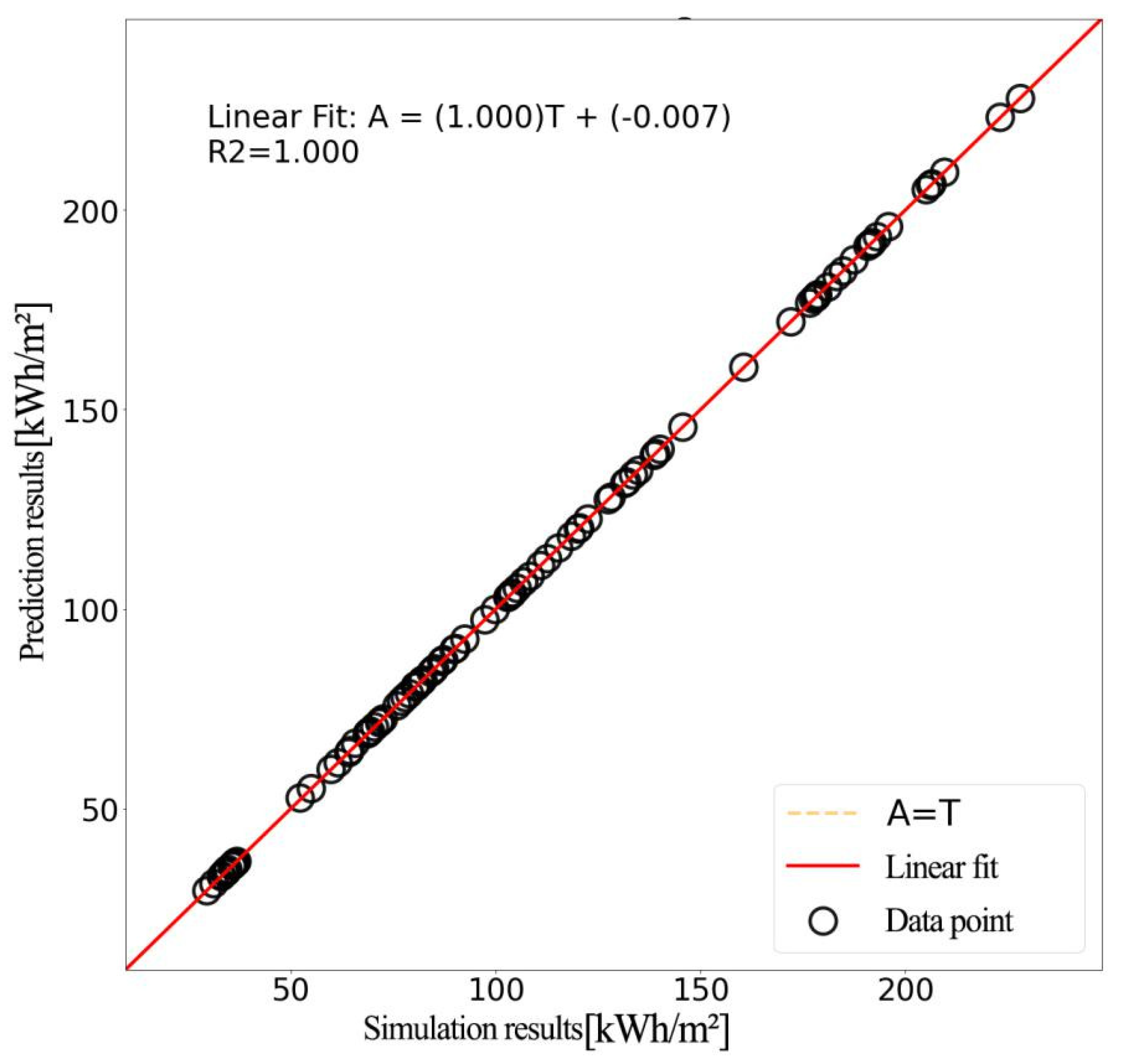
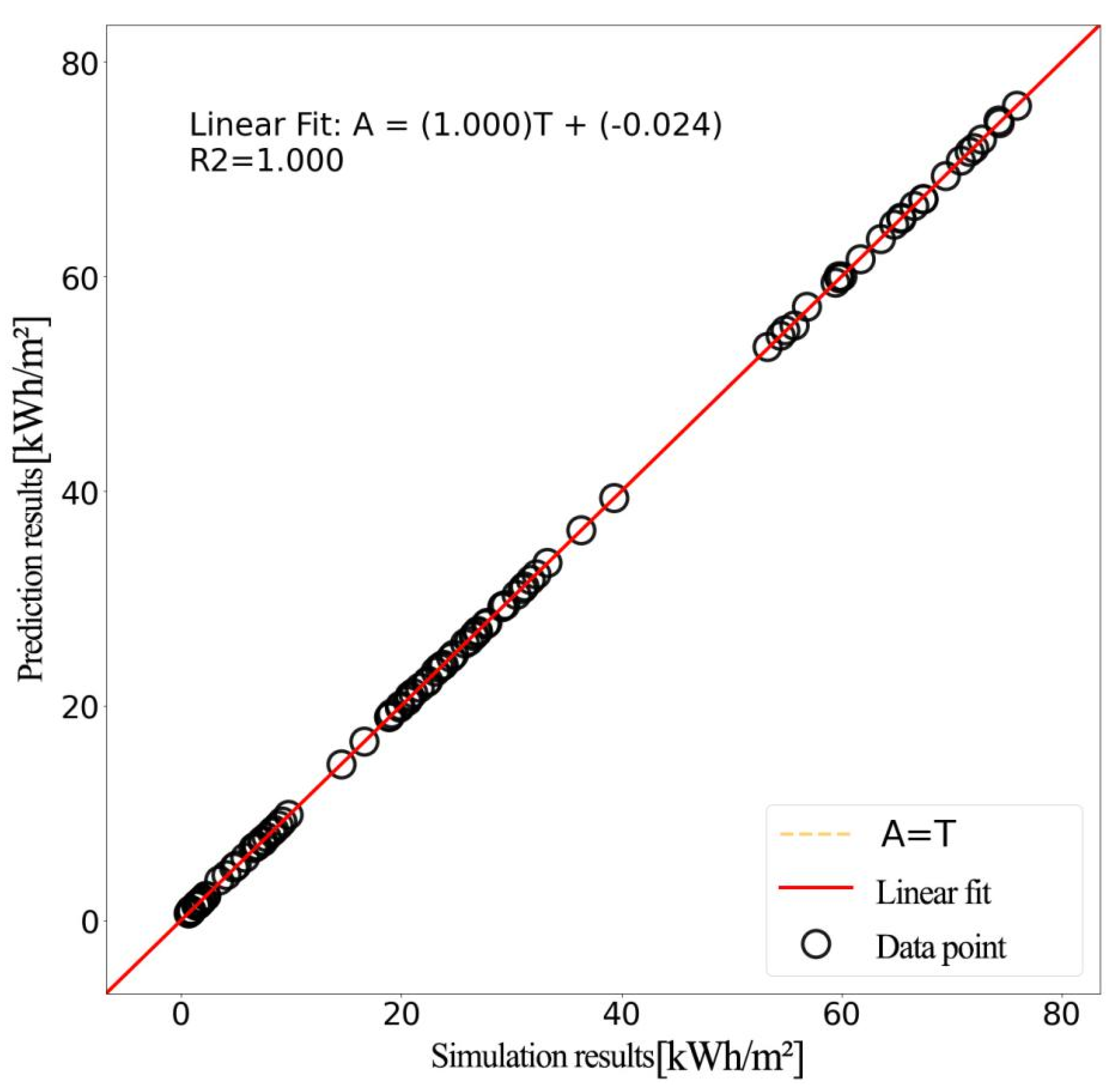
| Data Set | Data Type | MAE | MSE | R2 |
|---|---|---|---|---|
| Training set | Cooling demand | 0.067 | 0.012 | 1.000 |
| Heating demand | 0.056 | 0.007 | 1.000 | |
| Light environment (UDI index) | 0.261 | 0.207 | 0.996 | |
| Test set | Cooling demand | 0.072 | 0.009 | 1.000 |
| Heating demand | 0.059 | 0.006 | 1.000 | |
| Light environment (UDI index) | 0.318 | 0.304 | 0.994 |
| Classification | Code | Description | Harbin (Severe Cold Area I) | Beijing (Cold Regions II) | Shanghai (Hot Summer and Cold Winter Area III) | Shenzhen (Hot Summer and Warm Winter Area IV) | Kunming (Temperate Region V) | |||||
|---|---|---|---|---|---|---|---|---|---|---|---|---|
| nZEB(*) | UDI(*) | nZEB(*) | UDI(*) | nZEB(*) | UDI(*) | nZEB(*) | UDI(*) | nZEB(*) | UDI(*) | |||
| Spatial morphological parameters | A1 | Floor height | 2.70 | 2.70 | 2.70 | 2.70 | 2.70 | 2.70 | 2.70 | 2.70 | 2.70 | 2.70 |
| A2 | Total width | 14.97 | 14.96 | 14.97 | 14.97 | 12.28 | 14.98 | 14.98 | 14.90 | 11.20 | 14.92 | |
| A3 | Total depth | 7.88 | 7.89 | 7.88 | 7.88 | 9.61 | 7.88 | 7.88 | 7.92 | 10.54 | 7.91 | |
| A4 | Master bedroom width | 2.50 | 2.50 | 2.50 | 2.50 | 4.42 | 2.51 | 2.50 | 2.50 | 3.63 | 2.50 | |
| A5 | Master bedroom depth | 3.94 | 4.48 | 2.59 | 4.48 | 4.58 | 4.47 | 4.23 | 4.42 | 4.88 | 4.51 | |
| A6 | Middle bedroom width | 2.50 | 2.50 | 2.50 | 2.50 | 4.42 | 2.51 | 2.50 | 2.50 | 3.63 | 2.50 | |
| A7 | Middle bedroom depth | 2.24 | 1.70 | 3.60 | 1.70 | 3.18 | 1.70 | 1.88 | 1.73 | 3.89 | 1.70 | |
| A8 | North bedroom width | 2.50 | 2.50 | 2.50 | 2.50 | 4.42 | 2.51 | 2.50 | 2.50 | 3.63 | 2.50 | |
| A9 | North bedroom depth | 1.70 | 1.71 | 1.70 | 1.70 | 1.85 | 1.71 | 1.77 | 1.77 | 1.77 | 1.70 | |
| A10 | Kitchen width | 1.70 | 4.95 | 1.71 | 1.74 | 1.96 | 1.70 | 1.70 | 5.00 | 1.70 | 1.74 | |
| A11 | Kitchen depth | 1.70 | 1.71 | 1.70 | 1.70 | 1.85 | 1.71 | 1.77 | 1.77 | 1.77 | 1.70 | |
| Window parameters | B1 | Window-to-wall ratio in north bedroom | 0.15 | 0.16 | 0.15 | 0.27 | 0.29 | 0.26 | 0.15 | 0.18 | 0.15 | 0.15 |
| B2 | Window-to-wall ratio in middle bedroom | 0.15 | 0.15 | 0.15 | 0.15 | 0.15 | 0.15 | 0.15 | 0.15 | 0.15 | 0.15 | |
| B3 | Window-to-wall ratio in master bedroom | 0.19 | 0.15 | 0.41 | 0.15 | 0.49 | 0.32 | 0.18 | 0.16 | 0.15 | 0.36 | |
| B4 | Window-to-wall ratio in living room | 0.32 | 0.15 | 0.59 | 0.20 | 0.60 | 0.33 | 0.24 | 0.16 | 0.15 | 0.17 | |
| B5 | Window-to-wall ratio in Kitchen | 0.23 | 0.28 | 0.16 | 0.20 | 0.24 | 0.33 | 0.15 | 0.59 | 0.15 | 0.18 | |
| B6 | Window-to-wall ratio in dining room | 0.15 | 0.54 | 0.15 | 0.50 | 0.16 | 0.19 | 0.15 | 0.60 | 0.15 | 0.16 | |
| Objective Function | Harbin (Severe Cold Area I) | Beijing (Cold Regions II) | Shanghai (Hot Summer and Cold Winter Area III) | Shenzhen (Hot Summer and Warm Winter Area IV) | Kunming (Temperate Region V) | |||||
|---|---|---|---|---|---|---|---|---|---|---|
| nZEB(*) | UDI(*) | nZEB(*) | UDI(*) | nZEB(*) | UDI(*) | nZEB(*) | UDI(*) | nZEB(*) | UDI(*) | |
| BED (kWh/m2): Building energy demand | 84.36 | 91.23 | 110.69 | 137.48 | 24.86 | 29.47 | 63.57 | 70.08 | 23.69 | 28.85 |
| H (kWh/m2): Heating energy demand | 70.36 | 77.46 | 104.57 | 132.69 | 24.77 | 27.82 | 0 | 0 | 17.05 | 19.10 |
| C (kWh/m2): Cooling energy demand | 14.00 | 13.77 | 6.12 | 4.79 | 0.09 | 1.65 | 63.57 | 70.08 | 6.64 | 9.75 |
| UDI 100–2000 (%): Useful Daylight Illuminance | 80.27 | 82.92 | 71.43 | 78.99 | 67.49 | 88.84 | 87.06 | 89.24 | 71.56 | 87.19 |
| Objective Function | Harbin (Severe Cold Area I) | Beijing (Cold Regions II) | Shanghai (Hot Summer and Cold Winter Area III) | Shenzhen (Hot Summer and Warm Winter Area IV) | Kunming (Temperate Region V) | |||||
|---|---|---|---|---|---|---|---|---|---|---|
| nZEB(*) | UDI(*) | nZEB(*) | UDI(*) | nZEB(*) | UDI(*) | nZEB(*) | UDI(*) | nZEB(*) | UDI(*) | |
| BED (**) (kWh/m2): Building energy demand | 95.06 | 88.19 | 4.12 | −22.67 | 60.3 | 55.69 | 1.63 | −4.88 | 12.41 | 7.25 |
| H (**) (kWh/m2): Heating energy demand | 103.95 | 96.85 | −7.43 | −35.55 | 35.44 | 32.39 | 0 | 0 | 8.98 | 6.93 |
| C (**) (kWh/m2): Cooling energy demand | −8.89 | −8.66 | 11.55 | 12.88 | 24.86 | 23.3 | 1.63 | −4.88 | 3.43 | 0.1 |
| UDI 100–2000 (**) (%): Useful Daylight Illuminance | −23.69 | −26.34 | −11.68 | −19.24 | −6.74 | −28.09 | −22.39 | −24.57 | −4.56 | −20.19 |
Publisher’s Note: MDPI stays neutral with regard to jurisdictional claims in published maps and institutional affiliations. |
© 2022 by the authors. Licensee MDPI, Basel, Switzerland. This article is an open access article distributed under the terms and conditions of the Creative Commons Attribution (CC BY) license (https://creativecommons.org/licenses/by/4.0/).
Share and Cite
Li, Z.; Zou, Y.; Tian, M.; Ying, Y. Research on Optimization of Climate Responsive Indoor Space Design in Residential Buildings. Buildings 2022, 12, 59. https://doi.org/10.3390/buildings12010059
Li Z, Zou Y, Tian M, Ying Y. Research on Optimization of Climate Responsive Indoor Space Design in Residential Buildings. Buildings. 2022; 12(1):59. https://doi.org/10.3390/buildings12010059
Chicago/Turabian StyleLi, Zhixing, Yukai Zou, Mimi Tian, and Yuxi Ying. 2022. "Research on Optimization of Climate Responsive Indoor Space Design in Residential Buildings" Buildings 12, no. 1: 59. https://doi.org/10.3390/buildings12010059
APA StyleLi, Z., Zou, Y., Tian, M., & Ying, Y. (2022). Research on Optimization of Climate Responsive Indoor Space Design in Residential Buildings. Buildings, 12(1), 59. https://doi.org/10.3390/buildings12010059