Experimental, Analytical and Numerical Studies of Interfacial Bonding Properties between Silane-Coated Steel Fibres and Mortar

Abstract

A systematic investigation of the effects of silane coatings on steel fibre–mortar interfacial bond properties was conducted, combining pullout tests, analytical solutions, and meso-scale FE simulations. Nine silane coatings were tested, and their effects were evaluated by 30 single fibre pullout tests. They were found to increase the peak force and energy consumption up to 5.75 times and 2.48 times, respectively. Closed-form analytical solutions for pullout load, displacement, and interfacial stress distribution during the whole pullout process were derived based on a tri-linear bond-slip model, whose parameters were calibrated against the pullout tests. Finally, the calibrated bond-slip models were used to simulate the pullout tests and complex failure of multi-fibre specimens in mesoscale finite element models. Such an approach of combining pullout tests, analytical solutions, and mesoscale modelling provides a reliable way to investigate the effects of fibre–mortar interfacial properties on the mechanical behaviour of steel fibre reinforced concrete members in terms of structural strength, stiffness, ductility, and failure mechanisms.

1. Introduction

Plain concrete consists of aggregates, mortar, and pores, and its low tensile strength makes concrete structures susceptible to fracture and brittle failure. To overcome this weakness, fibres made from steel [1], polymer [2,3], carbon [4], glass [5] etc., are often added to reinforce the concrete. Steel fibres are the most widely used fibres to reinforce concrete in structural applications due to its easy access, recyclability, and reinforcement efficiency [6]. Steel fibre reinforced concrete (SFRC) has higher tensile/flexural/compressive/fatigue strengths, fracture toughness, and ductility than plain concrete [7,8,9,10] due to the crack-bridging effect of steel fibres, which delays crack initiation and propagation in concrete [11,12]. Such effect is mainly dependent on the interfacial bonding properties and energy dissipation between fibres and mortar during fibre pullout. Improving the interfacial properties between these two materials is, therefore, important for SFRC to achieve better macroscopic mechanical performances.

To date, substantial efforts have been made to enhance the interfacial properties between steel fibres and mortar, mainly adopting two techniques, i.e., using deformed fibres and modifying fibre–mortar interfaces. The deformed fibres include hooked-end, corrugated, waved, and twisted fibres and those with irregular shapes. Extra mechanical anchor forces are created as the deformed fibres are gradually pulled out from the mortar, compared with straight circular fibres. For example, hooked-end and corrugated steel fibres can increase the maximum pullout force by 2–6 times [13,14,15]. Twisted fibres were reported to provide stable higher pullout forces due to the untwisting process [16]. Arch-type [17,18] and spiral [19] steel fibres were also found to improve the interfacial bond strength by different levels. Meanwhile, improving the interfacial properties by modifying fibre surfaces has also attracted much attention. For example, He et al. [20] coated steel fibres by nano-scale iron oxide and found that the bond strength increased by 82% compared with conventional SFRC. Pi et al. [21] coated steel fibres with a nano-SiO₂ multilayer film and the interfacial bond strength increased by 77.5% and the pullout energy by 67.4%. Miller et al. [22] treated fibre surfaces using oxygen/argon plasma, resulting in a 25% increase in the peak load and a 34% increase in the pullout work. Other surface treatments such as using the zinc phosphate (ZnPh) [23,24,25] were also found to be able to improve the interfacial bond strength to different extents.

Silane is an inorganic compound and an excellent coupling agent widely used to coat metal plates for corrosion protection, such as steel [26,27], aluminium [28], and nickel–manganese–gallium (NiMnGa) alloy [29], in many industries. In the last two decades, silane coupling agents (SCA) are increasingly used to modify cementitious materials. For example, Kong et al. [30] tried three silane solutions to modify cement paste and mortar and found they could increase the flowability but did not necessarily benefit hydration and strength. Felekoglu [31] found that using the alkyl alkoxy silane to treat aggregate surfaces led to better workability and higher compressive strength of concrete. Cao et al. [32] found that adding silane into mortar can improve dispersion of steel fibres, and Ma [33] found that silane could increase the interfacial bond strength between cement paste and aggregates. Silane has also been sporadically used to coat different fibres. For example, Benzerzour et al. [34] treated recycled polyester fibres with vinyl trimethoxy silane and found that the fibre-cement pullout energy could be increased by three times. The same silane was applied in [35] on glass fibres, resulting in 1.86 times higher fibre–mortar bond strength than the untreated fibres. Callen et al. [36] used three types of silanes to treat stainless steel fibres used in the epoxy matrix and found 50% increase in the bending strength. Very recently, Liu et al. [37] tried the 3-aminopropyltriethoxysilane silane to coat steel fibres in an ultra-high performance concrete (UHPC) matrix, and found that the use of 5% SCA decreased flowability but increased the first crack load, the first crack displacement, and the energy absorption capacity by 12.4%, 57.8%, and 13.8% under bending loads, respectively. Using scanning electron microscope (SEM), they also found that the SCA films increased fibre surface roughness and interfacial friction and resulted in new chemical bonds and physical hydrophilic interactions that firmly adhered the UHPC matrix to the steel fibre surfaces. Casagrande et al. [38] carried out a similar study and found that the silane (tetraethoxysilane) coating on steel fibres increased the amount of calcium silicates hydrates (C-S-H) at the interface with the UHPC matrix; the average bond strength, measured by multi-fibre tension tests, was increased by 35.6% and the crack width at the peak load was reduced by 49.5%. This seems the only pullout experiment reported in the literature of SCA-coated steel fibres from cementitious materials.

The above review demonstrates that the silane coupling agents have great potentials to improve the interfacial bond behaviour between steel fibres and cementitious materials, but the research in this area has just started recently, and a systematic and in-depth investigation is still much needed. This study aims to systematically identify optimal silane coupling agents for coating steel fibres used in SFRC, by a combination of laboratory experiments, analytical analysis and numerical simulations. Nine types of silane solutions are designed, and their effectiveness is compared in terms of the load–displacement curves from 30 single fibre pullout tests. SEM tests are carried out to characterize and compare the microstructures of coated fibre surfaces and the interfacial transitional zones before and after fibre pullout. Furthermore, analytical solutions for the full-range pullout process are derived using a tri-linear softening interfacial bond-slip constitutive model, whose material parameters are calibrated against the pullout tests for each silane. These constitutive curves are then used in finite element (FE) simulations of the single fibre pullout tests and SFRC specimens with randomly distributed multiple steel fibres, to demonstrate the effects of different silane coatings on the structural strength and failure mechanisms.

2. Experiments

2.1. Materials

The mortar is made of ordinary Portland cement (grade P.O 42.5), fine sand, and water with the weight ratio of 1:1.2:0.41. The sand particle size ranges from 0.1 mm to 0.5 mm. The steel fibres were 1 mm in diameter, 1600 MPa in tensile strength and 200 GPa in Young’s modulus. Three groups of silane solutions were used: (a) Group Z (Z1–Z4) are four Dow Cornings^® silane-based coupling agents, including amino-propyl-tri-ethoxy-silane (Z6011), amino-propyl-tri-methoxy-silane (Z6020), methyl-propyl-acyloxy-propyl-trimethoxy-silane (Z6030), and glycidyl-ether-oxypropyl-trimethoxy-silane (Z6040); (b) Group ZZ (ZZ1–ZZ4) are compound solutions with the above four silane coupling agents added with Zr(NO₃)₄·5H₂O crystals; (c) Group ZH2 is the Z6020 solution mixed with H₂ZrF₆ solution (45% wt) since H₂ZrF₆ has notable effects on anti-corrosion of steel plates [39].

2.2. Coating Procedure and Specimen Fabrication

Silane coating of the steel fibres involves three steps: (1) Hydrolysis [37,38]: mix one portion of methanol, six portions of deionized water, and one portion of silane together and stir the solution at room temperature for 20 min, and then add a proper amount of acetic acid to adjust the PH value of the solution in the range of 4–6; wait for 24 h until the silane completely hydrolysed. The four silane coupling agents (Z6011, Z6020, Z6030, and Z6040) in group Z were produced first, and Zr(NO₃)₄ with concentration of 0.01 mol/L was then added to make the four solutions in Group ZZ. Group ZH2 was produced by adding H₂ZrF₆ (with 8% mass fraction of the final solution) into the Z6020 agent. (2) Pre-treatment of fibres: fibres were polished using sandpapers with fineness of 600 and 1500 to remove the oxide layer and original metal coating and were further cleaned using alkaline detergent to remove other impurities on the surface. They were subsequently soaked in sodium hydroxide solution of 20% (wt) for 30 min, rinsed by deionized water to remove the residual lye, and then immersed in anhydrous ethanol to remove the residual water film on the fibres’ surfaces and left to dry naturally. (3) Coating: the steel fibres were immersed in the silane-based coupling solutions and stirred gently for 2 min to ensure solution to be adsorbed onto the fibre surfaces. The fibres were then taken out and dried at a constant temperature of 110 °C for 30 min until the surface modification were completed. Untreated steel fibres of the same lengths were also prepared as the reference group.

The fine sand, cement, and water were prepared according to the designed mix proportion. After the cement and fine sand were dry-mixed for 2 min, half the water was added and mixed for 4 min, followed by addition of another half water and 8 min mixing. The mixture was then moved into a cylinder mould with a diameter of 68 mm and a height of 136 mm. A steel fibre was embedded in the cylinder centre with an embedment length of 40 mm, as shown in Figure 1. The steel fibre and the mould were fixed and vibrated for 1 min with a vibration frequency of 50 Hz. The specimen was then moved into a curing chamber with a temperature of 20 ± 1 °C and a relative humidity of 90% and were cured for 28 days. Three repeat specimens for each group, i.e., 30 specimens in total, were prepared. Meanwhile, three 70.7 mm mortar cubes were prepared under the same condition and tested according to the standard JCJ/T70-2009 [40]. The obtained average compressive strength at 28 days was 43.6 MPa with a standard deviation (SD) of 2.31 MPa.

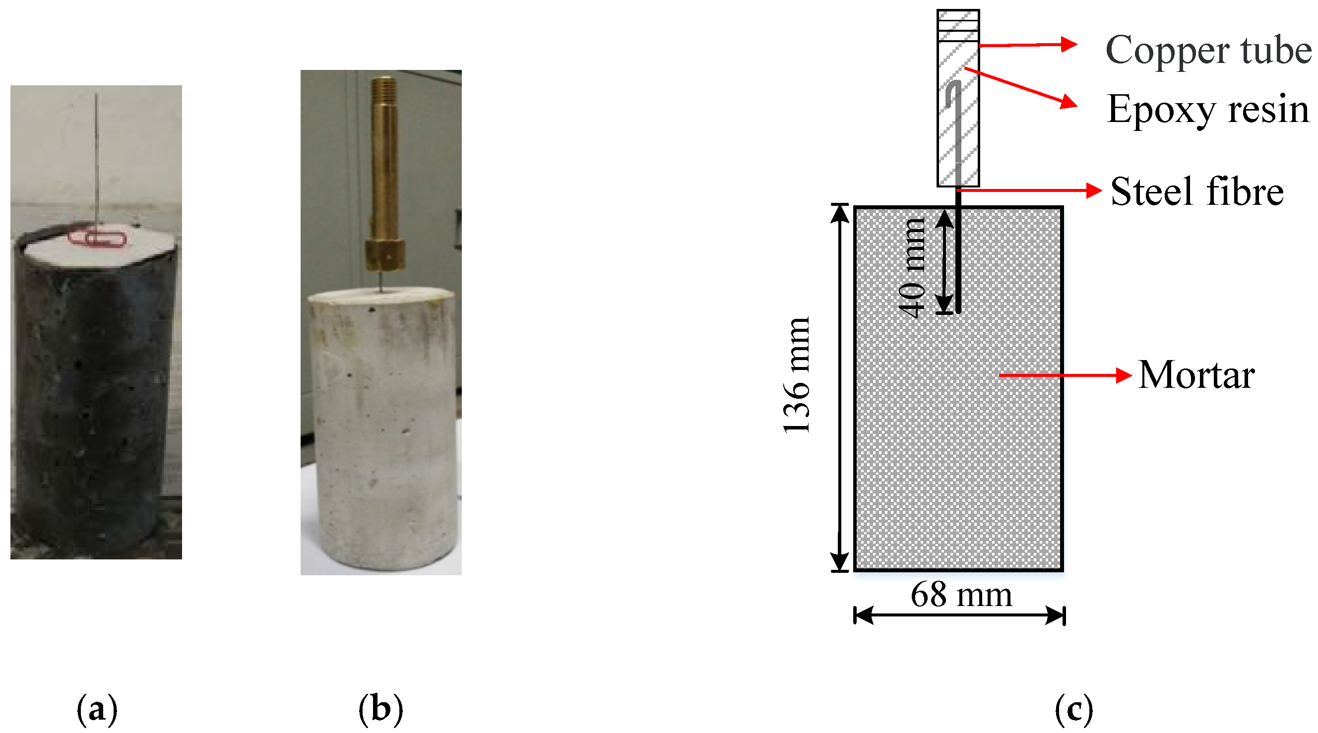
2.3. Single Fibre Pullout Tests

The test setup of single fibre pullout is similar to those used in [14,16,24]. As shown in Figure 1c, the exposed end of the steel fibre was bent at 45° and buried with a length of 50 mm in a copper pipe (12 mm in outer diameter, 10 mm in inner diameter and 100 mm in length) filled with epoxy resin to ensure that the pullout occurred in the mortar. After the epoxy resin was cured for 24 h, pullout tests were performed on an Instron 8802 test machine as shown in Figure 2. The specimen was fixed by a jack set between the specimen and the customized steel frame with the copper pipe passing through a reserved hole in the middle bottom of the steel frame. A force transducer with a measuring range/accuracy of 10 kN/0.5 N was connected with the copper pipe. The loading was controlled by displacement with a rate of 0.5 mm/min.

2.4. SEM Tests

The surfaces of steel fibres were scanned and analysed using a field emission environmental scanning electron microscopy (SEM: FEG650) and an energy spectrometer (EDS: EDAX), both supplied by FEI, USA. The scanned samples were 15 mm cubes that were cut perpendicular to the fibre axis in groups U and Z1 before the pullout tests. The sample surfaces were polished by a diamond grinding wheel and encapsulated in vacuum in transparent resin. The interfacial transition zones (ITZ) of fibre–mortar interfaces were also scanned and analysed using SEM.

3. Experimental Results and Discussion

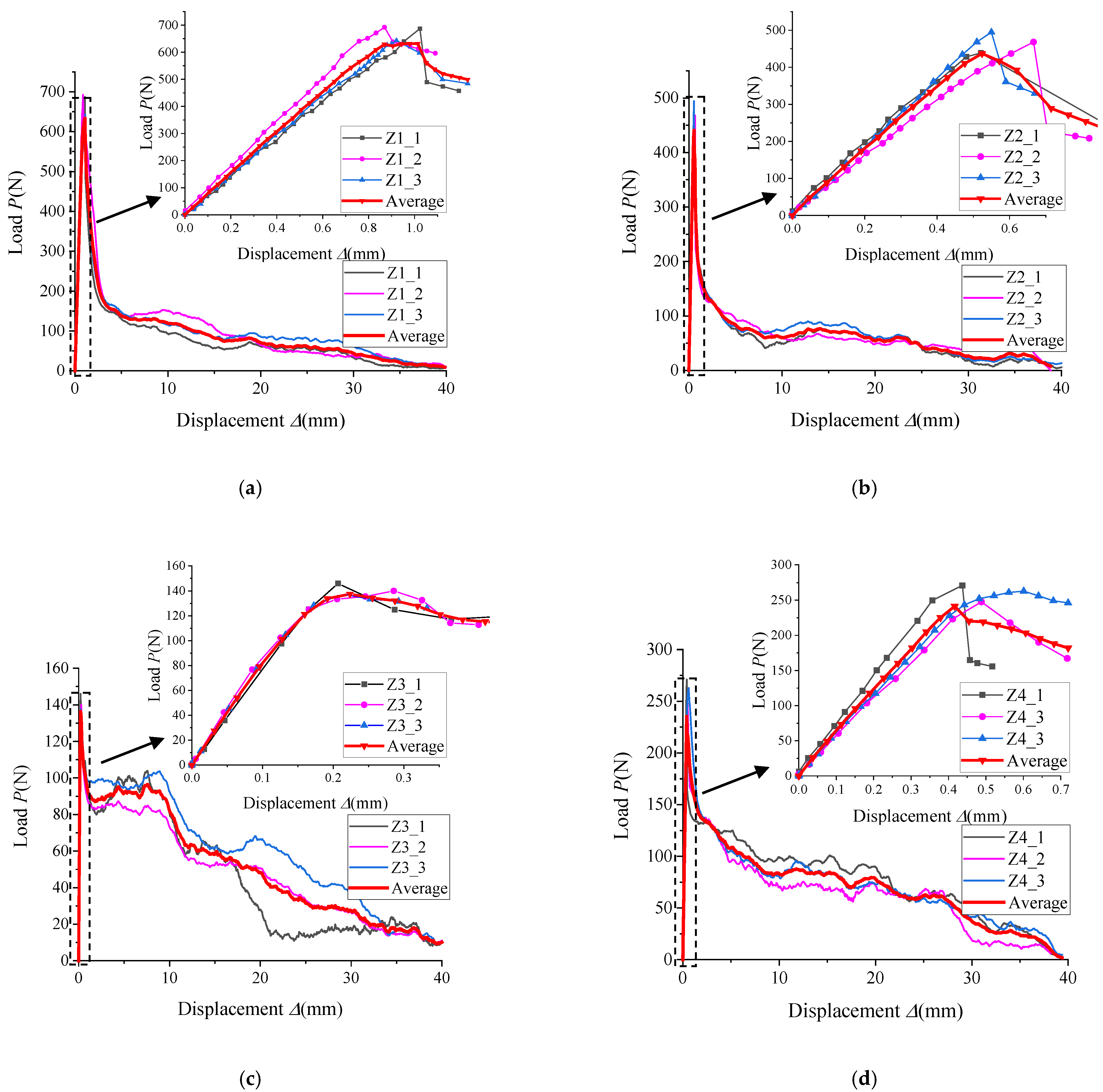
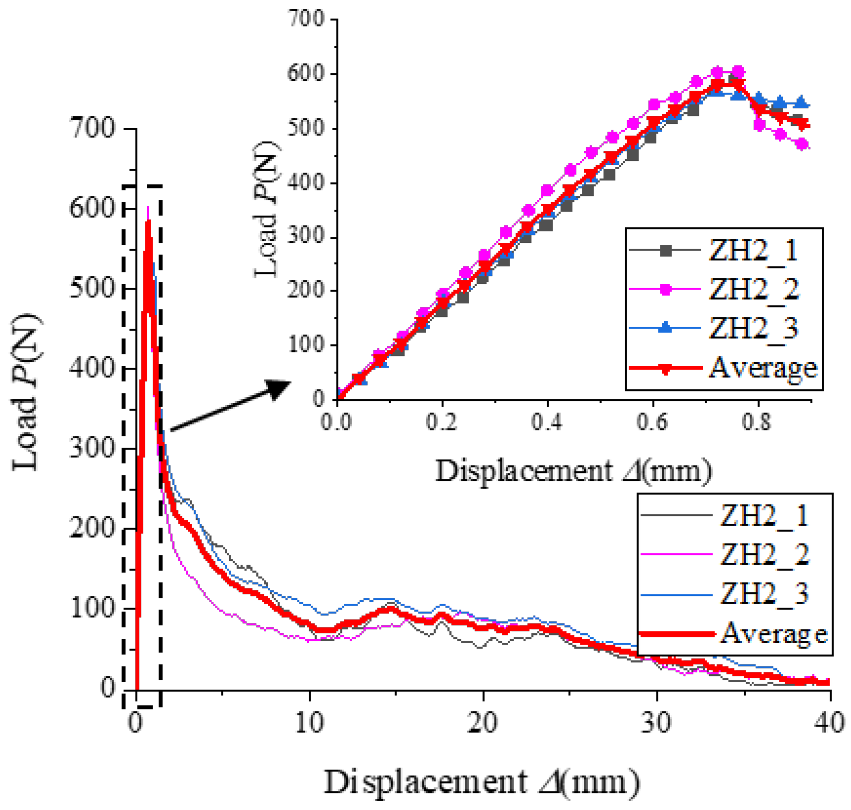
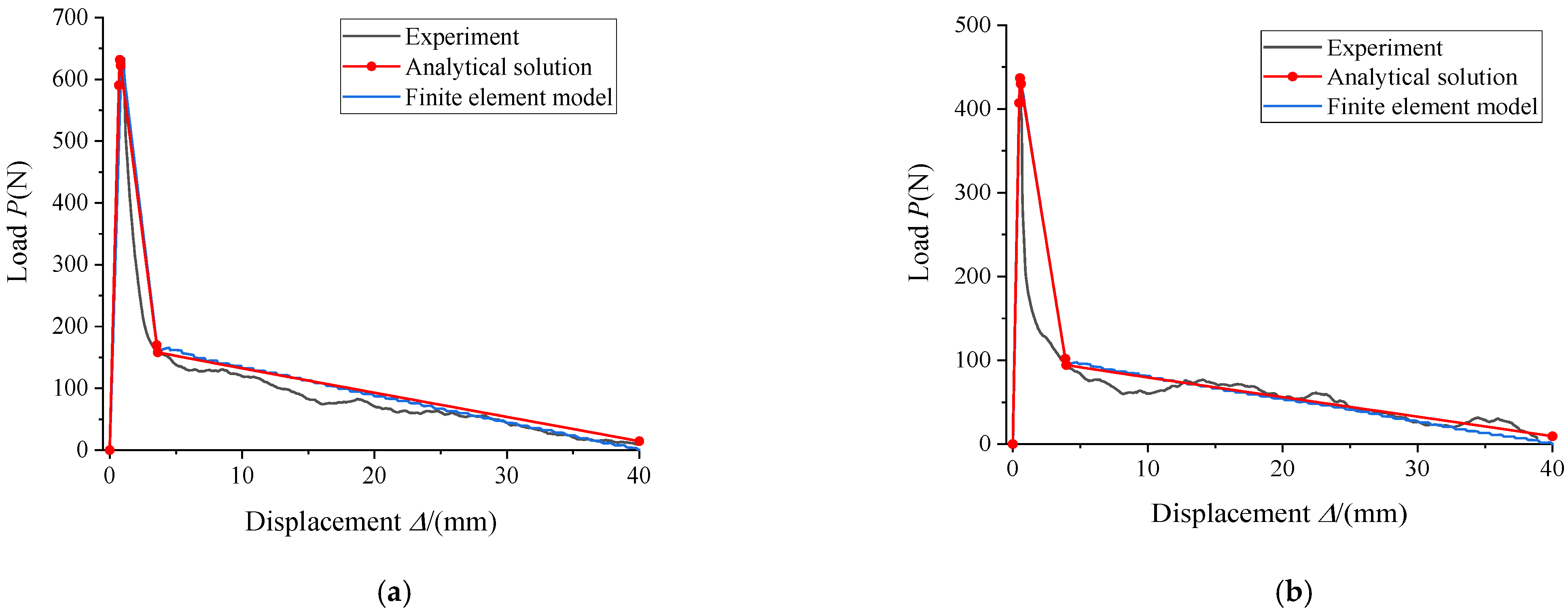
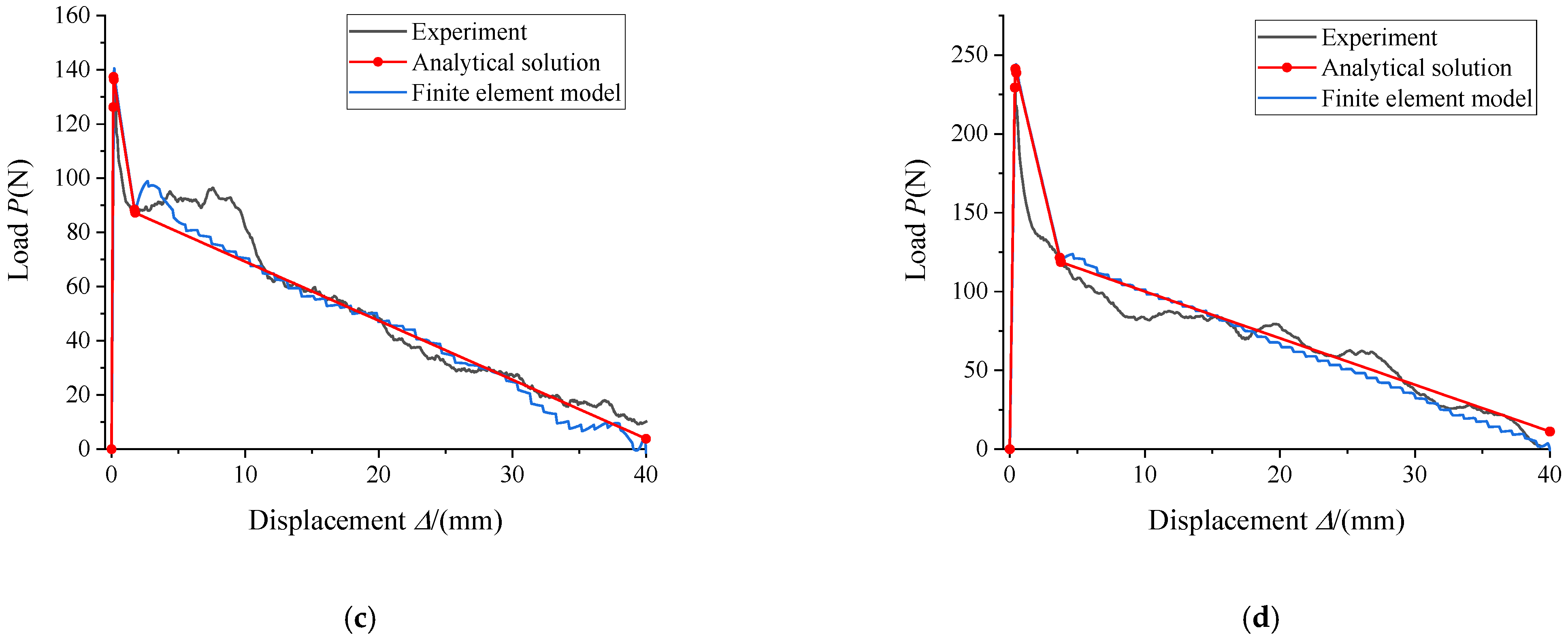
3.1. Pullout Load-Displacement (P-Δ) Curves and the Bond-Slip Process

Figure 3, Figure 4, Figure 5 and Figure 6 show the pullout load-displacement (P-Δ) curves, the mean-value curves, and the detailed curves around the peak load, for all the groups (Z, ZZ, ZH2, and U (untreated fibres)) of specimens. It should be noted that the scales of Y axis (loading) are very different. All these curves are typical to single fibre pullout tests and similar in shape to those reported in [14,41].

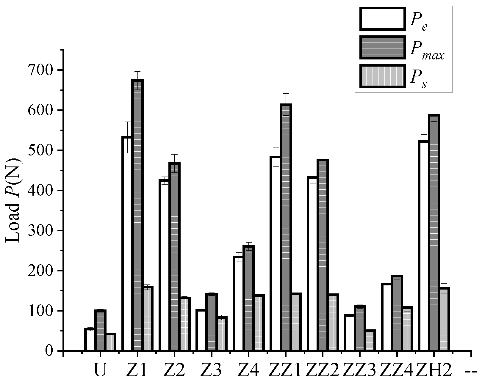
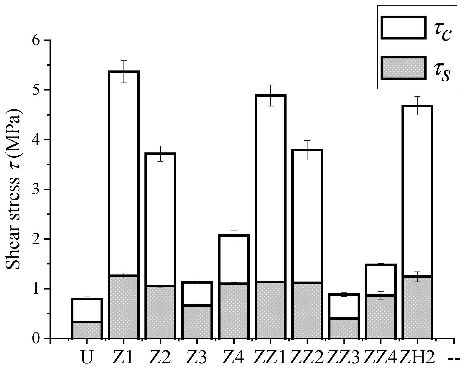
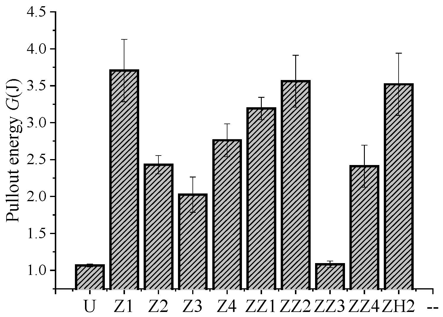
3.2. Parameters of Interfacial Bond Properties

To assess the effects of silane coatings on the interfacial behaviour, the following characteristic parameters are defined and extracted from the experiment P-Δ data:

$${\tau }_{max}=\frac{P_{max}}{2\pi r_{f}L}$$

(1)

$${\tau }_s=\frac{P_s}{2\pi r_{f}L}$$

(2)

$${\tau }_c={\tau }_{max}-{\tau }_s$$

(3)

$$G={\int }_0^{L}P\mathrm{d}l$$

(4)

where L and r_f are the initial embedment length and radius of fibres, respectively. P_max and P_s are the peak load and the load when the whole fibre is debonded from the mortar (only friction remains afterwards), respectively. τ_max is the interfacial bond strength corresponding to P_max based on the assumption of a uniform distribution of interfacial shear stress along the fibre [24]. τ_s is the residual frictional bonding strength at the end of the debonding process, without taking the fibre surface roughness into account. τ_c denotes the chemical bond strength, and G is the area under the P-Δ curve, representing the energy dissipated during the pullout process. The mean values of the above parameters of three specimens for each coating groups, together with the load at the end of elastic stage P_e, are summarized in

Table 1. Major parameters extracted from the pullout tests.

Group No.	Coating Types	Pe (N)	Pmax (N)	Ps (N)	τmax (MPa)	τc (MPa)	τs (MPa)	G (J)
U	Untreated	70.65	99.91	41.95	0.80	0.46	0.33	1.07
Z1	Z6011	546.88 (674%)	673.96 (575%)	158.95 (279%)	5.37 (575%)	4.10 (789%)	1.27 (279%)	3.71 (248%)
Z2	Z6020	407.25 (476%)	467.10 (368%)	132.35 (215%)	3.72 (368%)	2.67 (478%)	1.05 (215%)	2.43 (128%)
Z3	Z6030	126.11 (79%)	141.22 (41%)	83.22 (98%)	1.12 (41%)	0.46 (0.08%)	0.66 (98%)	2.02 (90%)
Z4	Z6040	233.74 (231%)	260.43 (161%)	138.57 (230%)	2.07 (161%)	0.97 (110%)	1.10 (230%)	2.76 (159%)
ZZ1	Z6011 + Zr(NO3)4	569.51 (706%)	613.84 (514%)	142.09 (239%)	4.89 (514%)	3.76 (714%)	1.13 (239%)	3.19 (200%)
ZZ2	Z6020 + Zr(NO3)4	404.70 (473%)	475.95 (376%)	140.37 (235%)	3.79 (376%)	2.67 (479%)	1.12 (235%)	3.56 (200%)
ZZ3	Z6030 + Zr(NO3)4	96.82 (37%)	110.83 (11%)	50.41 (20%)	0.88 (11%)	0.48 (4%)	0.40 (20%)	1.08 (2%)
ZZ4	Z6040 + Zr(NO3)4	174.03 (146%)	186.43 (87%)	108.25 (158%)	1.48 (87%)	0.62 (35%)	0.86 (158%)	2.41 (126%)
ZH2	Z6020 + H2ZrF6	522.34 (639%)	587.41 (488%)	156.05 (272%)	4.68 (488%)	3.43 (644%)	1.24 (272%)	3.52 (230%)

, where values in parentheses represent the increase percentages over the results in the U group. The data in Table 1 and their SDs are also presented in Figure 7, Figure 8, Figure 9 and Figure 10 for comparative analyses.

3.3. The Effects of Silane Coatings on the Interfacial Properties

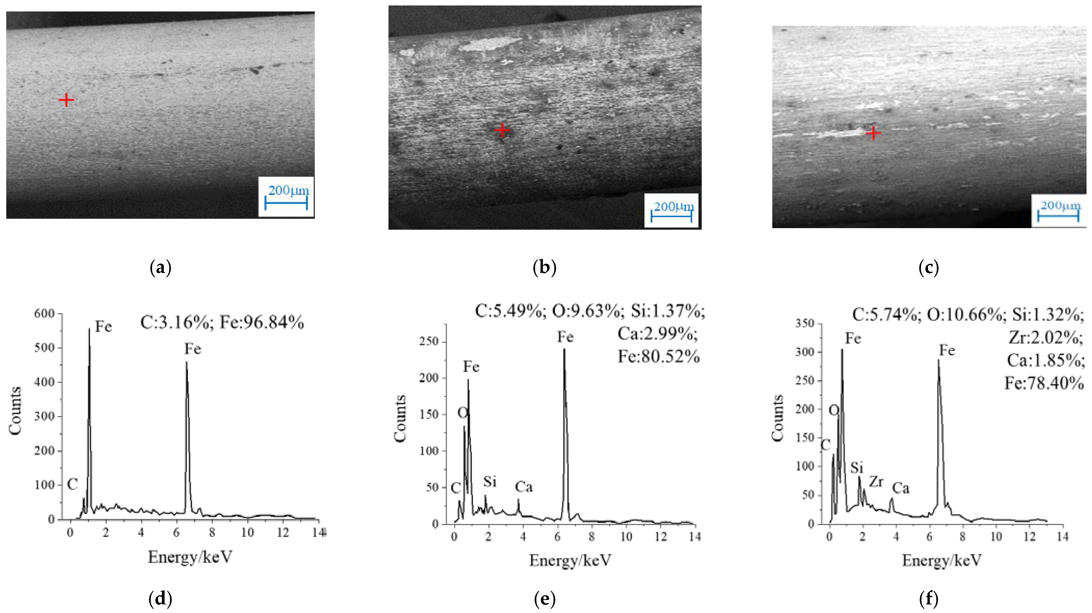
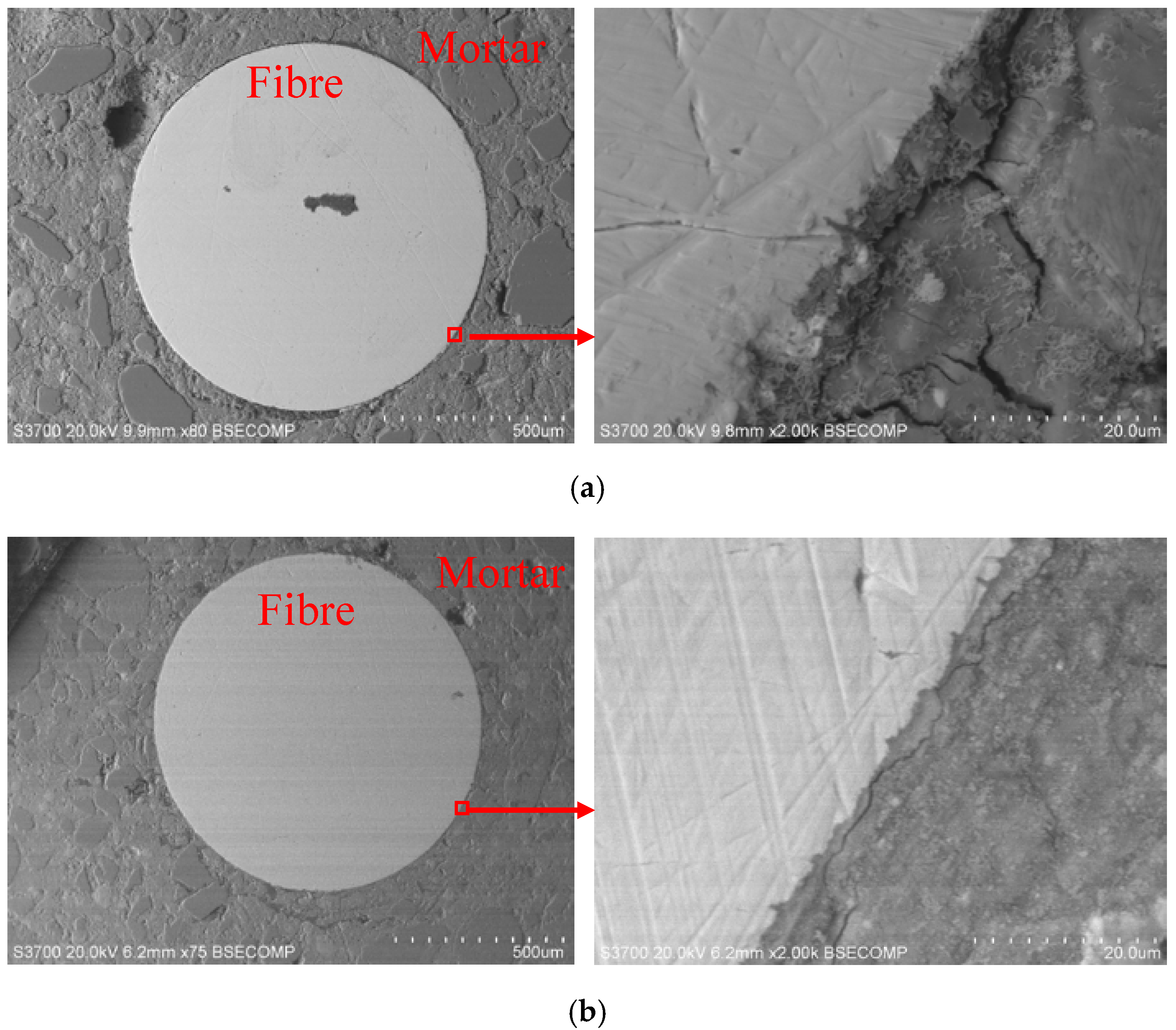
It can be seen from Table 1 that all of the interfacial bonding properties of coated fibres were improved compared with the untreated fibres. The peak pullout load P_max and the bond strength τ_max of specimens in Z1 and ZZ1 groups were increased by 575% and 514%, respectively; the increase percentage ranges from 368 to 488% for the groups of Z2, ZZ2, and ZH2, and is 161% and 87% for Z4 and ZZ4, respectively. The least improvement happened to the group Z3 (41%) and ZZ3 (11%), respectively. Similar trends can be found in the improvements of P_e, P_s (or τ_s), τ_c and G, ranging from 37 to 706%, 20 to 279%, 0.1 to 789%, and 2 to 248%, respectively.

As shown in Figure 8, the ratio of τ_c/τ_max was 0.59 for the untreated fibres. This ratio increased to 0.71–0.76 for the groups with Z6011 and Z6020 coatings (Z1, Z2, ZZ1, ZZ2, ZH2) but decreased to 0.41–0.55 for those with Z6030 and Z6040 coatings (Z3, Z4, ZZ3, ZZ4), indicating the former ones mainly enhanced the chemical bonding strength τ_c and the latter mainly increased the residual frictional bonding strength τ_s. Figure 9 compares the total pullout energy consumption G. Comparison of Figure 7 and Figure 9 indicates a strong correlation between G and P_max. The increased percentages over the untreated fibres for τ_max, τ_s, τ_c and G are plotted in Figure 10. In general, Z6011 (Z1 and ZZ1) performed the best, followed by Z6020 (Z2, ZZ2, and ZH2) and Z6040 (Z4 and ZZ4), while Z6030 (Z3 and ZZ3) was not effective. The first two groups with Z6011 and Z6020 had high increases in τ_max with the increased percentages Δτ_c > Δτ_max > Δτ_s, indicating these two silane agents mainly contributed to the increase in chemical bonding properties. The reverse situation can be seen for the latter two groups with Z6040 and Z6030, which mainly increased the interfacial friction. Furthermore, adding Zr(NO₃)₄ (group ZZ) weakened the interfacial properties (compared with group Z), while adding H₂ZrF₆ to Z6020 (group ZH2) performed better than Z6020 alone (group Z2).

3.4. SEM Tests

3.4.1. Surface Observation of Steel Fibres

Figure 11 presents the SEM micrographs and EDS energy spectra of steel fibres from the groups of U, Z1, and ZZ1 before the pullout tests. The fibre surface looks brighter than the silane coatings due to the steel’s higher reflectivity. The surface of the untreated fibre is smooth (Figure 11a) while those treated fibres are much rougher (Figure 11b,c). Figure 11d–f show that only Fe and C elements exist on the surface of untreated fibres, while additional elements of Si, O, and Ca were detected on the Z1-treated fibre surface and extra Zr and Ca elements were found on ZZ1-treated fibre surface. This suggests the existence of silane coatings and the effectiveness of the coating technique used.

The coating mechanism can be explained in chemical reactions. The chemical structure of silane molecules is represented by R-Si(OX)₃, where R represents carbon-chain functional groups that can react with organic compounds, such as carbonyl, amino, and epoxy; OX is a group that can react with H₂O and generate Si-OH, and X is commonly -CH₃, -C₂H₅, etc. According to the chemical bond theory [42], forming of silane coating on fibres involves four step chemical reactions: (1) hydrolysis: the Si-OX group is hydrolysed to Si-OH; (2) condensation: Si-OH is dehydrated and condensed into a multi-molecular structure; (3) hydrogen bonding: Si-OH in the oligomer forms a hydrogen bond with -OH on the surface of steel fibres; and (4) coating formation: a covalent bond is formed with the fibre along with the dehydration reaction during heating and curing. The rough silane coatings increase the contact area and form an anchorage effect between the steel fibres and the mortar matrix, leading to enhanced pullout responses in the treated fibres over the untreated (Figure 3, Figure 4, Figure 5 and Figure 6).

3.4.2. ITZ Observation

The SEM images of fibre–mortar interface transitional zones (ITZ) are shown in Figure 12a,b, for the untreated group U and treated group Z1, respectively. It is clearly visible that the interfacial microstructure was relatively loose and there existed some micro-cracks for the untreated specimen, probably caused by shrinkage from the highly different elastic moduli and thermal expansion coefficients of steel fibres and the mortar. On the contrary, the ITZ microstructure of the sample in the group Z1 is much denser with fewer micro-cracks of smaller width, probably due to enhanced hydration reactions by the silane coating and, thus, stronger and denser C-H-S materials around the ITZ, as reported in [37]. In addition to the anchorage effect described above, the densification of the ITZ due to the fibre treatment leads to higher bonding performances.

4. Analytical Solutions for the Full-Range Pullout Process

The experimental pullout force-displacement curves and the calculated interfacial properties from single fibre pullout tests are very useful to compare the effectiveness of different silane coatings. However, these curves are geometry and boundary dependent and are not material properties. Therefore, they cannot be used as the constitutive laws of the interface that are needed for the analysis and design of SFRC structures with many randomly distributed fibres. A direct measurement of the interfacial constitutive laws, namely, the interfacial stress–slip relations, involves careful setup of strain gauges along the fibres and is very difficult to conduct for such narrow steel fibres in mm or tenth of mm (e.g., for UHPFRC). Here, we developed an indirect method to characterize a simplified tri-linear softening interfacial bond-slip constitutive law, combining analytical solutions and parameter calibrations against the experimental pullout curves. Closed-form analytical solutions have been derived in our previous study [43] for the whole pullout process of rockbolts. Although mechanically very similar, the solutions in [43] are applicable for pullout problems with the embedment length of fibres/bars/rockbolts being longer than the effective embedment length (see Section 4.3), which is typically not the case for SFRC or UHPFRC with short fibres. A new set of analytical solutions are, thus, derived as below.

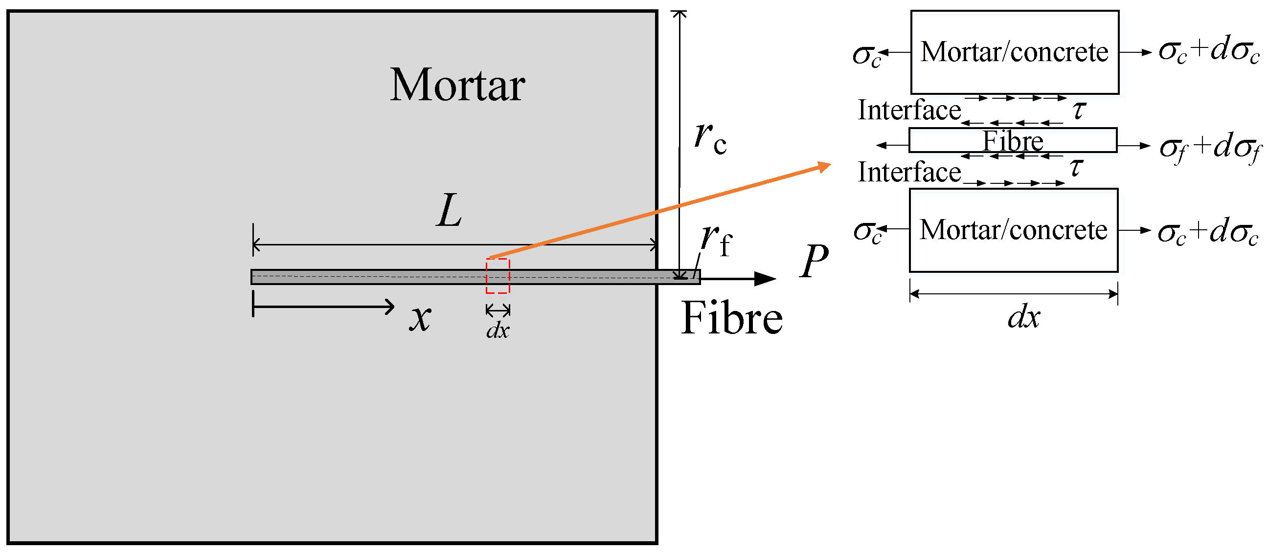
4.1. The Idealized Model and Assumptions

Figure 13 shows the idealized model of the single fibre pullout tests. The experimental results indicate that the ultimate failure in the pullout tests is debonding and pullout of a very thin layer of mortar attached in the critical interfacial zones. The deformation in this zone is assumed to be lumped into the zero-thickness fibre-matrix interface, thus, the mortar deformation outside this zone is neglected, due to the massive volume and stiffness of the surrounding mortar. The fibre-matrix interface is assumed to be under pure shear and the fibre is assumed to be under uniaxial tension. It is also assumed that the pullout force P is horizontal so that the stress in the protruding length of the fibre is uniform.

Based on the assumptions stated above, the governing equations can be established from force equilibrium considerations:

$$\frac{d{\sigma }_f}{dx}-\frac{2\tau }{r_f}=0$$

(5)

where τ is the shear stress at the interface, σ_f the axial stress in the fibre, x the axial coordinate along the fibre’s length with its origin at the embedment end and r_f the fibre radius. Assuming that the fibre remains linear elastic throughout the pullout process, the constitutive equation for the fibre is

$${\sigma }_f=E_f\frac{d{u}_f}{dx}=E_f\frac{d\delta }{dx}$$

(6)

where E_f is the Young’s modulus of the fibre, u_f is the axial displacement of the fibre and δ is the shear slip between the fibre and the mortar.

Substituting Equation (6) into Equation (5), the governing equation and the axial stress of the fibre are expressed as:

$$\frac{d^2\delta }{d{x}^2}-\frac{{\delta }_f}{{\tau }_f}{\lambda }^2\tau \left(\delta \right)=0$$

(7)

$${\sigma }_f=\frac{2{\tau }_f}{{\delta }_f{r}_f{\lambda }^2}\frac{d\delta }{dx}$$

(8)

where

$${\lambda }^2=\frac{2{\tau }_f}{{\delta }_f{E}_f{r}_f}$$

(9)

Equation (7) can be solved once the bond-slip model represented by τ(δ) is defined.

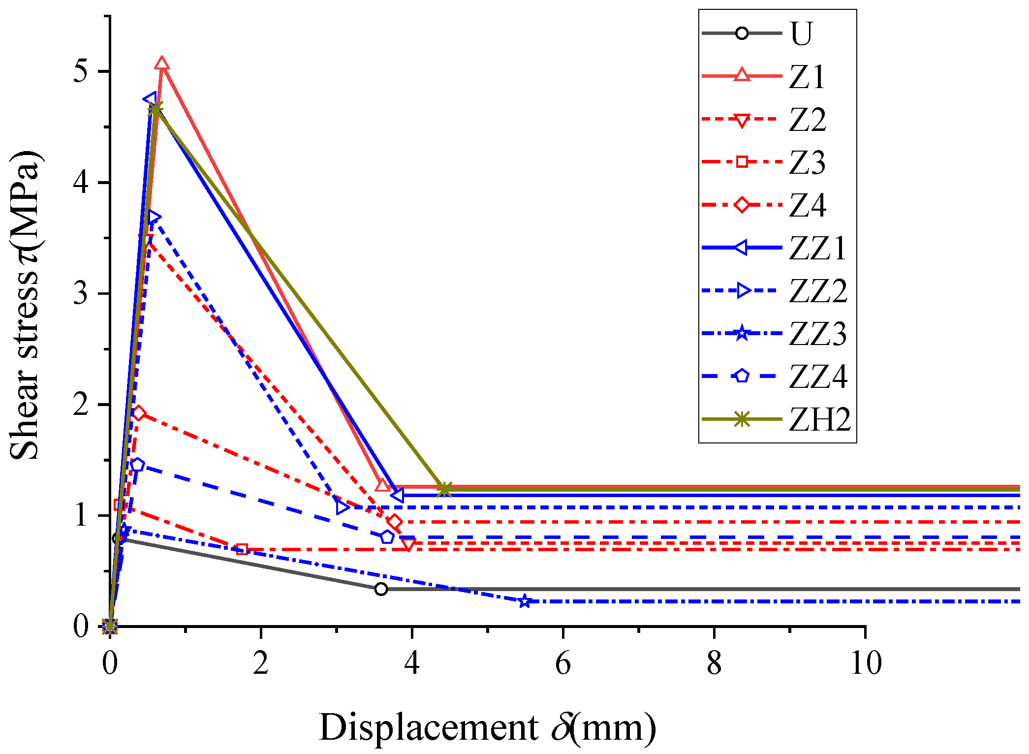
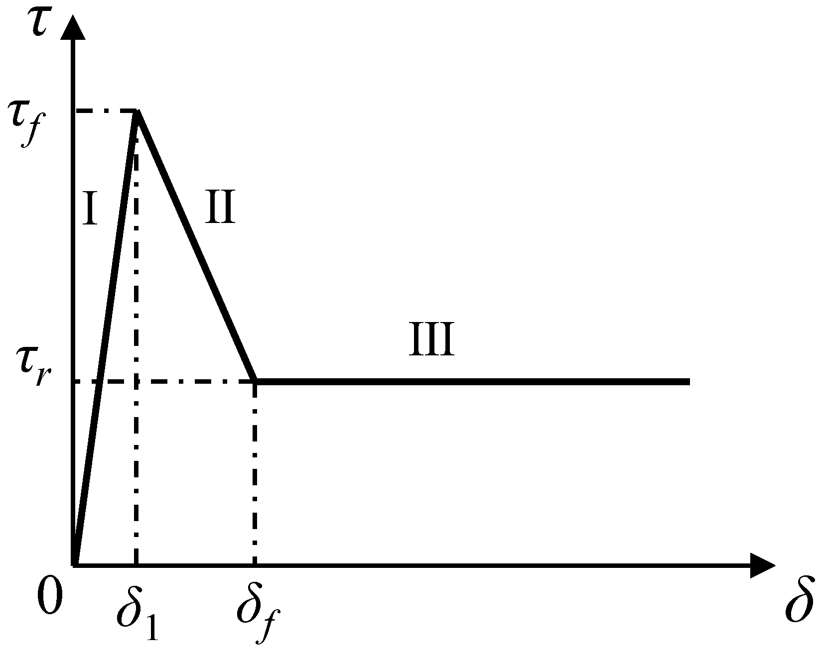
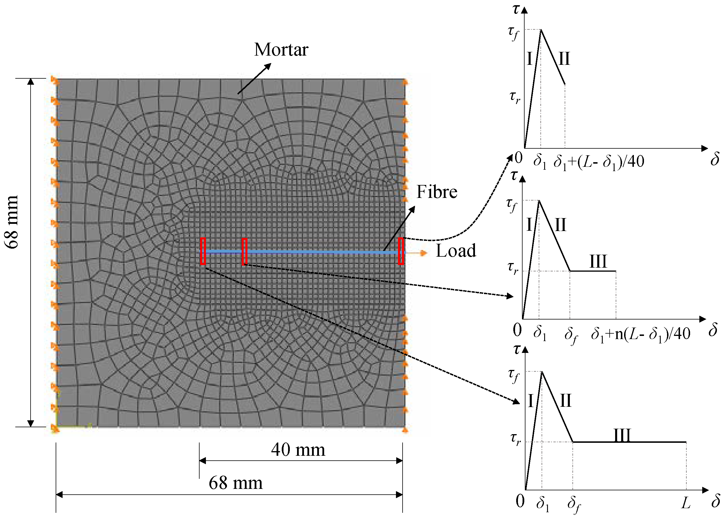
4.2. The Tri-Linear Bond-Slip Model

The same tri-linear bond-slip model as used for grout–rockbolt interfaces [43] and fibre reinforced concrete joints [44] was assumed as the interfacial constitutive law for the fibre–mortar interface. As illustrated in Figure 14, the model consists of an ascending linear elastic branch (I) up to the peak stress or bond strength at (δ₁, τ_f), followed by a softening branch (II) down to (δ_f, τ_r), and finally a horizontal branch (III) representing the non-zero residual frictional strength τ_r after complete debonding.

The equation for the bond-slip model is expressed as

$$\tau \left(\delta \right)=\{\begin{array}{cc}\begin{array}{ccc}\frac{{\tau }_f}{{\delta }_1}\delta & for& 0\le \delta \le {\delta }_1\\ \frac{k{\tau }_f\left(\delta -{\delta }_1\right)+{\tau }_f\left({\delta }_f-\delta \right)}{{\delta }_f-{\delta }_1}& for& {\delta }_1\le \delta \le {\delta }_f\\ k{\tau }_f& for& \delta \ge {\delta }_f\end{array}& \begin{array}{c}\begin{array}{c}\begin{array}{c}\left(a\right)\\ \\ \left(b\right)\end{array}\\ \end{array}\\ \left(c\right)\end{array}\end{array}$$

(10)

where k (0 ≤ k ≤ 1) is defined as the ratio of the residual shear strength τ_r and the bond strength τ_f. The tri-linear bond-slip model is assumed as a material property and all the parameters can be calibrated from pullout tests, as discussed later.

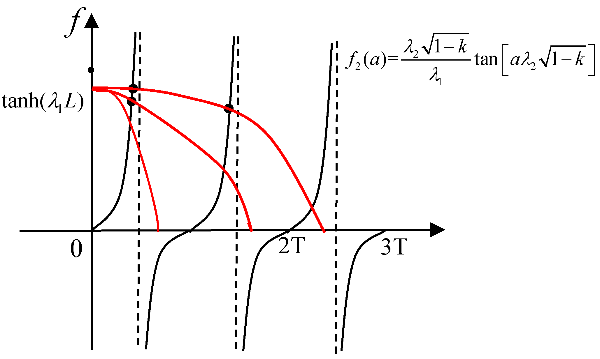
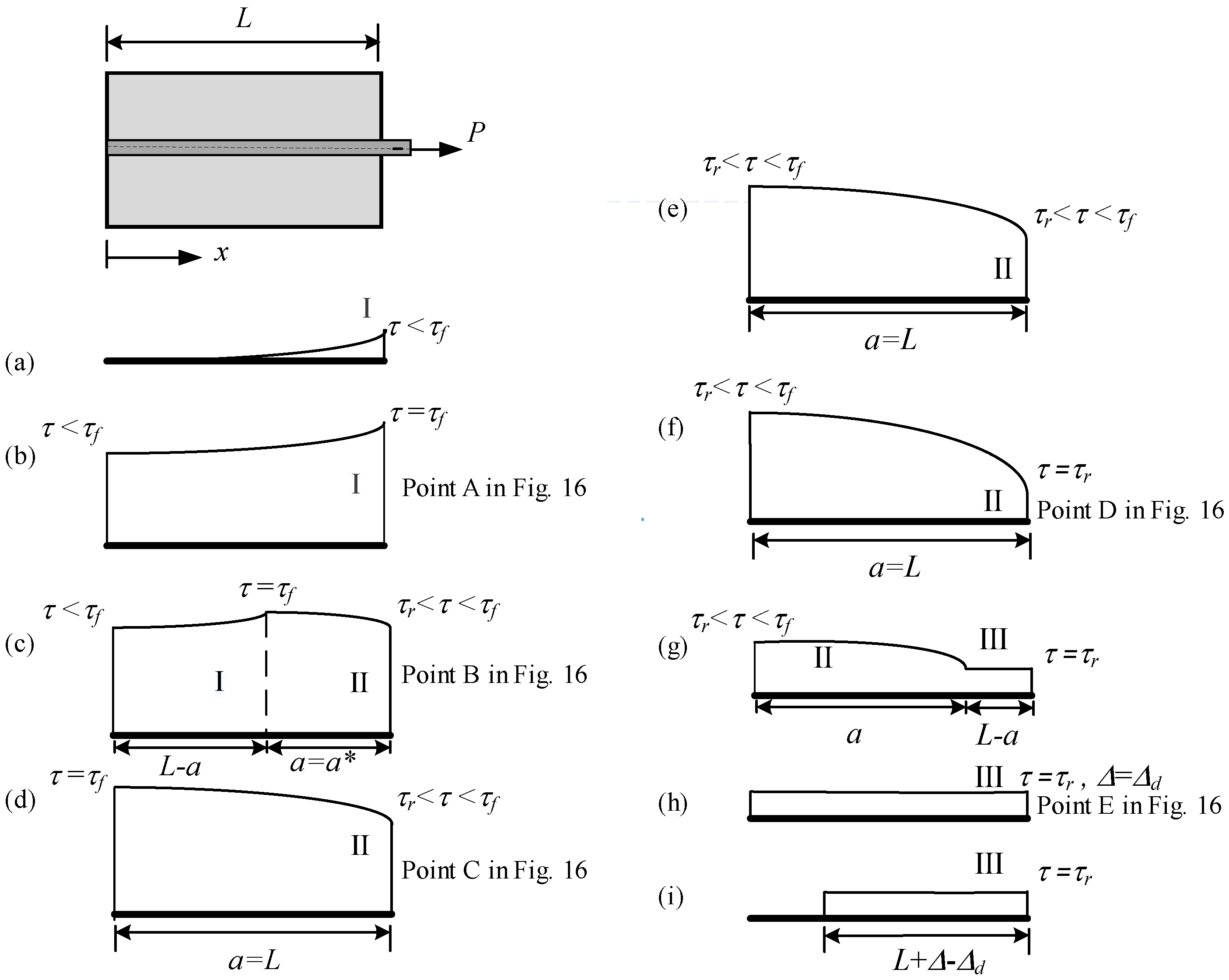
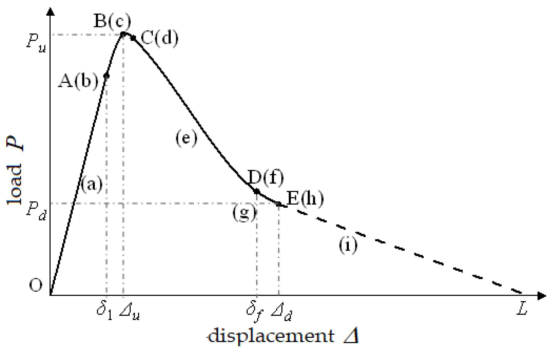
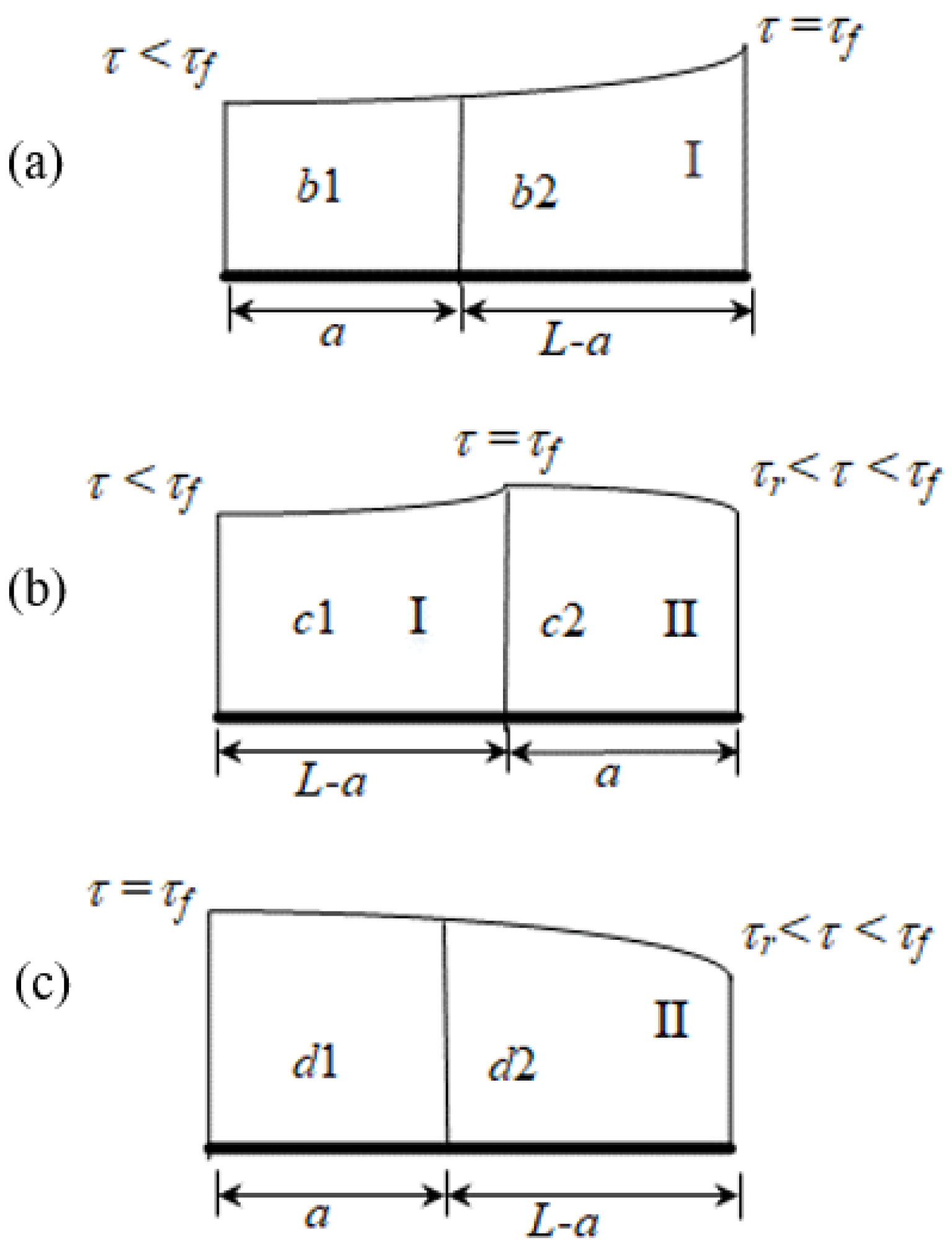
4.3. Analysis of the Full-Range Behaviour and Derivation of Analytical Solutions

Using the tri-linear bond-slip model defined above, the shear slip δ and shear stress τ distributions along the interface, the axial stress σ_f in the fibre, and the relation between load P—pulling end displacement Δ can be obtained by solving the governing equation Equation (7) for every loading stage. Figure 15 illustrates the five-stage evolution of interfacial shear stress distribution when the fibre embedment length is shorter than the effective embedment length l_e. It is significantly different from the evolution when the embedment length is much longer than l_e as in [43]. This leads to very different analytical solutions as derived below. Figure 16 shows the analytical load–displacement curve with the different stages in Figure 15 highlighted. It is not plotted up to scale for clarity.

4.3.1. Linear Elastic Stage (OA)

In this stage, the pullout force is low and the entire interface remains linear elastic (state I) until the interfacial shear stress at x = L reaches τ_f (Figure 15a,b and segment OA in Figure 16). Substituting Equation (10a) for 0 ≤ δ ≤ δ₁ into Equation (7), the differential equation for this stage can be obtained as

$$\frac{d{\delta }^2}{d{x}^2}-{\lambda }_1^2\delta =0$$

(11)

where

$${\lambda }_1^2=\frac{{\delta }_f}{{\delta }_1}{\lambda }^2=\frac{2{\tau }_f}{{\delta }_1{E}_f{r}_f}$$

(12)

Considering the boundary conditions in this stage:

$${\sigma }_f=0\mathrm{at}x=0$$

(13)

$${\sigma }_f=\frac{P}{\pi r_f^2}\mathrm{at}x=L$$

(14)

the interfacial slip, interfacial shear stress and axial stress in the fibre are obtained by solving the governing equation, Equation (11), as

$$\delta =\frac{{\delta }_{1}P{\lambda }_1\cosh ({\lambda }_{1}x)}{2\pi r_f{\tau }_f\sinh ({\lambda }_{1}L)}$$

(15)

$$\tau =\frac{P{\lambda }_1\cosh ({\lambda }_{1}x)}{2\pi r_f\sinh ({\lambda }_{1}L)}$$

(16)

$${\sigma }_f=\frac{P\sinh ({\lambda }_{1}x)}{\pi r_f^2\sinh ({\lambda }_{1}L)}$$

(17)

The slip at the loading end with x = L is defined as the fibre displacement, denoted as Δ. The following load–displacement expression can be obtained from Equation (15)

$$P=\frac{2\pi r_f{\tau }_f\tanh ({\lambda }_{1}L)}{{\lambda }_1{\delta }_1}\Delta$$

(18)

As in [43], the effective bond length is defined as the bond length over which the shear stresses offer a total resistance at least 97% of the applied load for an infinite bond length. Based on this definition and considering that tanh(2) ≈ 0.97, the effective bond length in the elastic stage is given by l_e = 2/λ₁. The embedment length is generally less than l_e for the steel fibres in SFRC, as will be shown later (

Table 2. Calibrated interfacial parameters.

ID	δ1 (mm)	τf (MPa)	δf (mm)	τr (MPa)	k	a* (mm)	le (mm)	Analytical Pu (N)	Test PB (N)	|Pu − PB|/PB (%)
U	0.12	0.79	3.59	0.34	0.43	39.14	172.50	99.44	99.46	0.019
Z1	0.69	5.06	3.61	1.26	0.25	33.64	164.89	631.74	631.68	0.009
Z2	0.48	3.49	3.95	0.75	0.22	35.93	165.24	436.80	436.74	0.014
Z3	0.13	1.10	1.75	0.70	0.63	38.57	152.69	137.48	137.42	0.043
Z4	0.38	1.92	3.77	0.94	0.49	37.51	198.47	241.30	241.28	0.010
ZZ1	0.55	4.75	3.83	1.18	0.25	35.26	152.10	593.69	593.73	0.007
ZZ2	0.57	3.69	3.06	1.08	0.29	34.06	175.52	461.12	461.16	0.007
ZZ3	0.19	0.87	5.49	0.23	0.26	38.91	208.48	109.66	109.63	0.024
ZZ4	0.37	1.46	3.67	0.80	0.55	37.75	223.91	182.75	182.78	0.016
ZH2	0.60	4.66	4.42	1.23	0.26	35.59	160.68	583.13	583.07	0.010

).

Equation (18) indicates that P increases proportionally with Δ in the elastic stage, which ends when Δ = δ₁ (Point A in Figure 16 and τ = τ_f in Figure 15b).

4.3.2. Elastic Softening Stage (ABC)

As the pullout force continues to increase, the shear stress at the loaded end (x = L) starts to decrease and the softening stage begins. The peak shear stress τ_f moves towards the embedment end, and a part of the interface near the loaded end enters the softening state (state II), as shown in Figure 15c. When the shear stress at the embedment end reaches τ_f, this stage is complete (Figure 15d and Point C in Figure 16).

During the elastic-softening stage, the following differential equations are obtained by substituting Equation (10a) and Equation (10b) into Equation (7):

$$\frac{d^2\delta }{d{x}^2}-{\lambda }_1^2\delta =0\mathrm{when}0\le \delta \le {\delta }_1$$

(19)

$$\frac{d^2\delta }{d{x}^2}+\left(1-k\right){\lambda }_2^2\delta ={\lambda }_2^2\left({\delta }_f-k{\delta }_1\right)\mathrm{when}{\delta }_1\le \delta \le {\delta }_f$$

(20)

where

$${\lambda }_2{}^2=\frac{{\delta }_f}{{\delta }_f-{\delta }_1}{\lambda }^2=\frac{2{\tau }_f}{\left({\delta }_f-{\delta }_1\right)E_f{r}_f}$$

(21)

The boundary conditions are

$${\sigma }_f=0\mathrm{at}x=0$$

(22)

$${\sigma }_f\mathrm{is}\mathrm{continuous}\mathrm{at}x=L-a$$

(23)

$$\delta ={\delta }_1\mathrm{and}\tau ={\tau }_f\mathrm{at}x=L-a$$

(24)

$${\sigma }_f=\frac{P}{\pi r_f^2}\mathrm{at}x=L$$

(25)

The solutions for the elastic region of the interface with 0 ≤ δ ≤ δ₁ (or 0 ≤ x ≤ L − a) are:

$$\delta =\frac{{\delta }_1\cosh ({\lambda }_{1}x)}{\cosh [{\lambda }_1\left(L-a\right)]}$$

(26)

$$\tau =\frac{{\tau }_f\cosh ({\lambda }_{1}x)}{\cosh [{\lambda }_1\left(L-a\right)]}$$

(27)

$${\sigma }_f=\frac{{\tau }_f\sinh ({\lambda }_{1}x)}{\cosh [{\lambda }_1\left(L-a\right)]}$$

(28)

where a is the length of the softening region.

The solutions for the softening region with δ₁ ≤ δ ≤ δ_f (or L − a ≤ x ≤ L) are:

$$\delta =\left({\delta }_f-{\delta }_1\right)\left\{\frac{{\lambda }_2\sin [{\lambda }_2\sqrt{1-k}\left(x-L+a\right)\left]\tanh [{\lambda }_1\left(L-a\right)\right]}{{\lambda }_1\sqrt{1-k}}-\frac{\cos [{\lambda }_2\sqrt{1-k}\left(x-L+a\right)]}{1-k}+\frac{{\delta }_f-k{\delta }_1}{\left(1-k\right)\left({\delta }_f-{\delta }_1\right)}\right\}$$

(29)

$$\tau =-{\tau }_f\left\{\frac{{\lambda }_2\sqrt{1-k}}{{\lambda }_1}\sin [{\lambda }_2\sqrt{1-k}\left(x-L+a\right)\left]\tanh [{\lambda }_1\left(L-a\right)\right]-\cos \left[{\lambda }_2\sqrt{1-k}\left(x-L+a\right)\right]\right\}$$

(30)

$${\sigma }_f=\frac{2{\tau }_f}{{\lambda }_2{r}_f\sqrt{1-k}}\left\{\frac{{\lambda }_2\sqrt{1-k}}{{\lambda }_1}\cos [{\lambda }_2\sqrt{1-k}\left(x-L+a\right)\left]\tanh [{\lambda }_1\left(L-a\right)\right]+\sin \left[{\lambda }_2\sqrt{1-k}\left(x-L+a\right)\right]\right\}$$

(31)

The applied load is obtained as:

$$P=\frac{2\pi r_f{\tau }_f}{\sqrt{1-k}{\lambda }_2}\left\{\frac{\sqrt{1-k}{\lambda }_2}{{\lambda }_1}\cos (a{\lambda }_2\sqrt{1-k})\tanh [{\lambda }_1\left(L-a\right)]+\sin (a{\lambda }_2\sqrt{1-k})\right\}$$

(32)

The displacement at x = L can be obtained as

$$\Delta =\left({\delta }_f-{\delta }_1\right)\left\{\frac{{\lambda }_2\sin (a{\lambda }_2\sqrt{1-k})\tanh [{\lambda }_1\left(L-a\right)]}{{\lambda }_1\sqrt{1-k}}-\frac{\cos (a{\lambda }_2\sqrt{1-k})}{1-k}+\frac{{\delta }_f-k{\delta }_1}{\left(1-k\right)\left({\delta }_f-{\delta }_1\right)}\right\}$$

(33)

To derive the peak force during this stage, the evolution of shear stress in Figure 15b–d are redrawn in Figure 17, where the areas enclosed by τ and the x-axis consist of two segments (a and L − a). They are denoted as A_b1, A_b2, A_c1, A_c2, A_d1, and A_d2, respectively, with A_c1 = A_b2 and A_c2 = A_d1. As the evolution is continuous, there must exist a a short enough to make A_c2 > A_b1, so A_c > A_b with A_b = A_b1 + A_b2 and A_c = A_c1 + A_c2. Similarly, there must exist a long enough a (a < L) to make A_c1 > A_d2, so A_c > A_d with A_d = A_d1 + A_d2. Therefore, there must exist an intermediate a = a* (0 < a* < L) that results in the highest area, which corresponds to the peak pullout force at point B in Figure 16.

The value of a* can be identified by making the derivative of Equation (32) with respect to a zero:

$$\frac{\partial P}{\partial a}=\frac{2\pi r_f{\tau }_f}{{\lambda }_1}\tanh \left[{\lambda }_1\left(L-a\right)\right]\left\{{\lambda }_1\cos (a{\lambda }_2\sqrt{1-k})\tanh [{\lambda }_1\left(L-a\right)]-{\lambda }_2\sqrt{1-k}\sin (a{\lambda }_2\sqrt{1-k})\right\}=0$$

(34)

This means either

$$\tanh [{\lambda }_1\left(L-a\right)]=0$$

(35)

or

$$\tanh [{\lambda }_1\left(L-a\right)]=\frac{{\lambda }_2\sqrt{1-k}}{{\lambda }_1}\tan (a{\lambda }_2\sqrt{1-k})$$

(36)

The solution of Equation (35) is a* = L, which is invalid because of a* < L based on the above analysis. However, an analytical solution to Equation (36) is difficult to obtain. Define

$$f_1\left(a\right)=\tan \mathrm{h}\left[{\lambda }_1\left(L-a\right)\right]$$

(37)

$$f_2\left(a\right)=\frac{{\lambda }_2\sqrt{1-k}}{{\lambda }_1}\tan \left[a{\lambda }_2\sqrt{1-k}\right]$$

(38)

Equation (36) becomes f₁(a) = f₂(a). The function f₁(a) decreases monotonously for 0 < a < L from 1 to zero and f₂(a) is a periodic function with a period of $\mathrm{T}=\pi /\left({\lambda }_2\sqrt{1-k}\right)$. The two functions are plotted on the a-f plane in Figure 18. The number of solutions to f₁(a) = f₂(a), namely, the intersection points between them, is dependent on the value of L and T. It is not difficult to find that for (n − 1)T< L ≤ nT where n is a positive integer, there are n number of intersection points in the range [0, L].

The period T of f₂(a) can be estimated considering the physical parameters of the materials used in the experiments. The magnitude (in the international standard unit system) of τ_f, δ_f − δ₁, E_f and r_f is in the order of 10⁶ Pa, 10⁻³ m, 10¹¹ Pa and 10⁻⁴ m, respectively, so λ₂² is in the order of 10² from Equation (21), that is, 1 < λ₂ < 10. Therefore, $\mathrm{T}=\pi /\left({\lambda }_2\sqrt{1-k}\right)$ is higher than π/10 = 0.314 m, considering 0 < k < 1. The embedment length of steel fibres in this study is L = 0.04 m, which is much lower than T. This also applies to SFRC and UHPFRC materials, which rarely use steel fibres longer than 40 mm in engineering practice. Therefore, there must be only one solution a = a* in the range of (0, L) for f₁(a) = f₂(a) or Equation (36).

The value of a* will be obtained using a simple numerical procedure given in 4.4. The peak force P_u and corresponding displacement Δ_u at point B in Figure 16 become

$$P_u=\frac{2\pi r_f{\tau }_f}{\sqrt{1-k}{\lambda }_2}\left\{\frac{{\lambda }_2\sqrt{1-k}}{{\lambda }_1}\cos ({\lambda }_2{a}^{*}\sqrt{1-k})\tanh [{\lambda }_1\left(L-a^{*}\right)]+\sin ({\lambda }_2{a}^{*}\sqrt{1-k})\right\}$$

(39)

$${\Delta }_u=\left({\delta }_f-{\delta }_1\right)\left\{\frac{{\lambda }_2\sin ({\lambda }_2{a}^{*}\sqrt{1-k})\tanh [{\lambda }_1\left(L-a^{*}\right)]}{{\lambda }_1\sqrt{1-k}}-\frac{\cos ({\lambda }_2{a}^{*}\sqrt{1-k})}{1-k}+\frac{{\delta }_f-k{\delta }_1}{\left(1-k\right)\left({\delta }_f-{\delta }_1\right)}\right\}$$

(40)

This stage ends at Figure 15d or point C in Figure 16 and the force and displacement can be calculated by substituting a = L into Equation (32) and Equation (33), respectively.

4.3.3. Softening Stage (CD)

In this stage, the entire interface enters softening (state II), as illustrated in Figure 15e–f and represented by the segment CD in Figure 16. The differential equation can be obtained by substituting Equation (10b) into Equation (7)

$$\frac{d^2\delta }{d{x}^2}+\left(1-k\right){\lambda }_2^2\delta ={\lambda }_2^2\left({\delta }_f-k{\delta }_1\right)$$

(41)

The general solution of Equation (41) is:

$$\delta ={\mathrm{C}}_1\cos ({\lambda }_{2}x\sqrt{1-k})+{\mathrm{C}}_2\sin ({\lambda }_{2}x\sqrt{1-k})$$

(42)

Defining the slip at the embedment end as δ₀, the boundary conditions are:

δ = δ₀ at x= 0

(43)

$${\sigma }_f=\frac{2{\tau }_f}{{\delta }_f{r}_f{\lambda }^2}\frac{d\delta }{dx}=0\mathrm{at}x=0$$

(44)

$${\sigma }_f=\frac{P}{\pi r_f^2}\mathrm{at}x=L$$

(45)

The solutions are:

$$\delta =\left({\delta }_0-\frac{{\delta }_f-k{\delta }_1}{1-k}\right)\cos ({\lambda }_2\sqrt{1-k}x)+\frac{{\delta }_f-k{\delta }_1}{1-k}$$

(46)

$$\tau =\frac{{\tau }_f\left[{\delta }_f-k{\delta }_1-\left(1-k\right){\delta }_0\right]}{{\delta }_f-{\delta }_1}\cos ({\lambda }_2\sqrt{1-k}x)$$

(47)

$${\sigma }_f=\frac{2{\tau }_f\sqrt{1-k}}{\left({\delta }_f-{\delta }_1\right)r_s{\lambda }_2}\left(\frac{{\delta }_f-k{\delta }_1}{1-k}-{\delta }_0\right)\sin ({\lambda }_2\sqrt{1-k}x)$$

(48)

Substituting Equation (45) into Equation (48) gives

$$P=\frac{2\pi r_s{\tau }_f\sqrt{1-k}}{\left({\delta }_f-{\delta }_1\right){\lambda }_2}\left(\frac{{\delta }_f-k{\delta }_1}{1-k}-{\delta }_0\right)\sin ({\lambda }_{2}L\sqrt{1-k})$$

(49)

The displacement at x = L can be obtained from Equation (46) as

$$\Delta =\left({\delta }_0-\frac{{\delta }_f-k{\delta }_1}{1-k}\right)\cos ({\lambda }_{2}L\sqrt{1-k})+\frac{{\delta }_f-k{\delta }_1}{1-k}$$

(50)

The range of the variable δ₀ (slip at the embedment end) in Equations (46)–(50) needs to be defined. At the beginning of this stage (Figure 15d or point C in Figure 16), the shear stress at the embedment end reaches τ_f with δ₀ = δ₁. At the end of this stage (Figure 15f and the point D in Figure 16), the shear stress at the loaded end decreases to τ_r with the slip equal to δ_f. Substituting τ = τ_r and δ = δ_f into Equation (46) leads to

$${\delta }_0=\frac{{\delta }_f-k{\delta }_1}{1-k}-\frac{k\left({\delta }_f-{\delta }_1\right)}{\left(1-k\right)\cos ({\lambda }_{2}L\sqrt{1-k})}$$

(51)

Therefore, the range of the variable δ₀ in this stage is

$${\delta }_1\le {\delta }_0\le \frac{{\delta }_f-k{\delta }_1}{1-k}-\frac{k\left({\delta }_f-{\delta }_1\right)}{\left(1-k\right)\cos ({\lambda }_{2}L\sqrt{1-k})}$$

(52)

which now fully defines Equations (46)–(50). Equations (49) and (50) indicate that the pulling force P decreases monotonically with both δ₀ and Δ.

4.3.4. Softening-Debonding Stage (DE)

This stage starts when δ = δ_f and τ = τ_r at the loaded end (x = L), with the shear stress distribution shown in Figure 15f (Point D in Figure 16). Debonding with residual friction shear strength (τ_r) only then initiates at the loaded end and moves towards the embedment end, until the whole interface is debonded at the point E in Figure 16. In this stage, the softening part is governed by Equation (41) and the debonding part is governed by

$$\frac{d^2\delta }{d{x}^2}-{\delta }_f{\lambda }^{2}k=0$$

(53)

which is obtained by substituting Equation (10c) into Equation (7). Equation (41) and Equation (53) can be solved considering the following boundary conditions:

$${\sigma }_f=0\mathrm{at}x=0$$

(54)

$${\sigma }_f\mathrm{is}\mathrm{continuous}\mathrm{at}x=a$$

(55)

$$\delta ={\delta }_f\mathrm{and}\tau =k{\tau }_f\mathrm{at}x=a$$

(56)

$${\sigma }_f=\frac{P}{\pi r_f^2}\mathrm{at}x=L$$

(57)

The solutions for the softening region with 0 ≤ x ≤ a are

$$\delta =\frac{k\left({\delta }_1-{\delta }_f\right)}{\left(1-k\right)\cos ({\lambda }_{2}a\sqrt{1-k})}\cos ({\lambda }_{2}x\sqrt{1-k})+\frac{{\delta }_f-k{\delta }_1}{1-k}$$

(58)

$${\sigma }_f=\frac{2k{\tau }_f}{{\lambda }_2{r}_f\sqrt{1-k}\cos ({\lambda }_{2}a\sqrt{1-k})}\sin ({\lambda }_{2}x\sqrt{1-k})$$

(59)

$$\tau =\frac{k{\tau }_f}{\cos ({\lambda }_{2}a\sqrt{1-k})}\cos ({\lambda }_{2}x\sqrt{1-k})$$

(60)

The solutions for the debonding region with L − a ≤ x ≤ L are

$$\delta =\frac{1}{2}k{\delta }_f{\lambda }^2\left(x-a{)}^2+\frac{k{\lambda }_2\left({\delta }_f-{\delta }_1\right)\left(x-a\right)}{\sqrt{1-k}}\tan ({\lambda }_{2}a\sqrt{1-k}\right)+{\delta }_f$$

(61)

$$\tau =k{\tau }_f$$

(62)

$${\sigma }_f=\frac{2{\tau }_f}{{\delta }_f{r}_f{\lambda }^2}\left[k{\delta }_f{\lambda }^{2}x+\frac{k{\lambda }_2\left({\delta }_f-{\delta }_1\right)}{\sqrt{1-k}}\tan ({\lambda }_{2}a\sqrt{1-k})-k{\delta }_f{\lambda }^{2}a\right]$$

(63)

The applied load P is obtained from Equation (63) at x = L as

$$P=\frac{2\pi r_f{\tau }_f}{{\delta }_f{\lambda }^2}\left[k{\delta }_f{\lambda }^{2}L+\frac{k{\lambda }_2\left({\delta }_f-{\delta }_1\right)}{\sqrt{1-k}}\tan ({\lambda }_{2}a\sqrt{1-k})-k{\delta }_f{\lambda }^{2}a\right]$$

(64)

The displacement can be obtained from Equation (61) at x = L as

$$\Delta =\frac{1}{2}k{\delta }_f{\lambda }^2\left(L-a{)}^2+\frac{k{\lambda }_2\left({\delta }_f-{\delta }_1\right)\left(L-a\right)}{\sqrt{1-k}}\tan ({\lambda }_{2}a\sqrt{1-k}\right)+{\delta }_f$$

(65)

Substituting a = 0 into Equations (64) and (65), there are

$$P_d=2\pi k{r}_f{\tau }_{f}L$$

(66)

$${\Delta }_d=\frac{1}{2}k{\delta }_f{\lambda }^2{L}^2+{\delta }_f$$

(67)

where P_d and Δ_d are the load and displacement at the pulling end when the whole interface is debonded, as shown in Figure 15h (point E in Figure 16).

4.3.5. Frictional Stage (EF)

In this stage, the shear resistance is provided by the residual interfacial friction strength τ_r only (Figure 15i). The shear stress is a constant

$$\tau =k{\tau }_f$$

(68)

The pullout displacement Δ varies from Δ_d at the beginning of this stage to L when the fibre is completely pulled out. Neglecting the fibre elongation, which is very small compared with Δ, the load–displacement relationship in this stage can be expressed as

$$P=2k\pi r_f{\tau }_f\left(L+{\Delta }_d-\Delta \right)$$

(69)

Equation (69) indicates that P reduces linearly to zero with Δ, as shown by the segment EF in Figure 16.

4.4. Calibration of Control Parameters

With the above analytical solutions available, the four parameters δ₁, τ_f, δ_f, and τ_r (or k) of the tri-linear bond-slip model in Figure 14 can now be calibrated against pullout experimental data of three control points A(Δ_A, P_A), B(Δ_B, P_B) and E(Δ_E, P_E) in Figure 16. These points are chosen because A is the end of the linear elastic stage, B is the peak point, and E is the starting point of the straight line EF, and they can all be easily identified on a pullout experimental curve.

From Figure 15b, it is clear that δ₁ = Δ_A. Substituting δ₁ = Δ_A, P_d = P_E and Δ_d = Δ_E into Equations (66)–(67), we get:

$${\delta }_f={\Delta }_E-\frac{P_{E}L}{2\pi E_f{r}_f^2}$$

(70)

$$k=\frac{P_{\mathrm{E}}}{2\pi r_{f}L{\tau }_f}$$

(71)

Substituting δ₁ = Δ_A and Equations (70) and (71) into Equation (36) and (39) (P_u = P_B) in the second stage (elastic-softening) leads to two equations with two unknown variables ${\tau }_f$ and a*, which are difficult to solve analytically. Herein, a simple numerical procedure is used. As seen in Figure 15, the variation of the interface shear stress along short steel fibres is not significant in this stage. It is reasonable (and safe) to assume that it ranges from zero to three times the interfacial bond strength τ_max calculated from Equation (1) at the peak point B (P_max = P_B). The range of τ_f∈[0,3τ_max] is divided into N number of equal intervals (N = 10,000 used for high accuracy herein). For each τ_fi = i(3τ_max/N) with i = 1~N, Equation (36) is solved to get a_i* using the function fsolve() in MatLab R2019b. τ_fi and a_i* are then substituted into Equation (39). If the calculated |P_u − P_B|/P_B ≤ 10⁻³, then τ_{f =} τ_fi is found as the solution; or otherwise, another loop is carried out with i= i + 1 until the convergence condition is met. Once τ_f is solved, k is calculated by Equation (71) and the full tri-linear bond-slip model is calibrated.

Table 2 summarises the calibrated parameters for all the ten groups of interfaces and the tri-linear bond-slip models are compared in Figure 19. It can be seen that at the peak load, the corresponding a* is quite close to the embedment length L = 0.04 m, which means the peak point B is close to the point C (Figure 16). The differences between the analytical peak loads and the experimental data are within 0.05% for all the tests, indicating the high accuracy of the numerical solutions (τ_f and a*) to Equation (39). It can also be seen that all types of silane coatings increase the bond strength τ_f except the ZZ3 group, with the Z1, ZZ1, and ZH2 groups being the most effective in enhancing both the bond strength τ_f and the residual strength τ_r. This is highly consistent with the test data analysis in 3.3 and proves that the silane-coating improves the interfacial bond-slip properties, which are indeed the underlying physical/chemical mechanisms for the improved pullout structural behaviour.

5. Numerical Simulations

The calibrated bond-slip models in Figure 19 can now be used as constitutive laws of the interfaces in finite element simulations of SFRC materials and structures. The single fibre pullout tests are modelled first as a validation of the FE modelling approach and the bond-slip laws, followed by simulations of direct tensile tests of an SFRC plate with randomly distributed fibres, as an application. In the FE models, the mortar is simulated by the continuum damage plasticity model in ABAQUS 6.13 [45] and fibres by elastoplastic beam elements. The fibre–mortar interfaces are modelled as zero-thickness cohesive elements (COH2D4), which are inserted between the steel fibres and the mortar. The developed tri-linear bond-slip laws in Figure 19 are used as the constitutive relations of the cohesive elements, with the damage index defined by Equation (72). In this way, all the deformation/failure modes such as fibre bending and breakage, mortar cracking, spalling and crushing, and interfacial bond-slip behaviour, can all be simulated in one model. The details of this discrete continuum coupled modelling approach can be referred to [46]. The FE simulations are conducted by the ABAQUS/Explicit solver with displacement control at the pulling end.

$$D=\{\begin{array}{cc}\frac{\left({\delta }_f-k{\delta }_1\right)\left(\delta -{\delta }_1\right)}{\left({\delta }_f-{\delta }_1\right)\delta }& {\delta }_1<\delta <{\delta }_f\\ 1-\frac{k{\delta }_1}{\delta }& {\delta }_f<\delta <L\end{array}$$

(72)

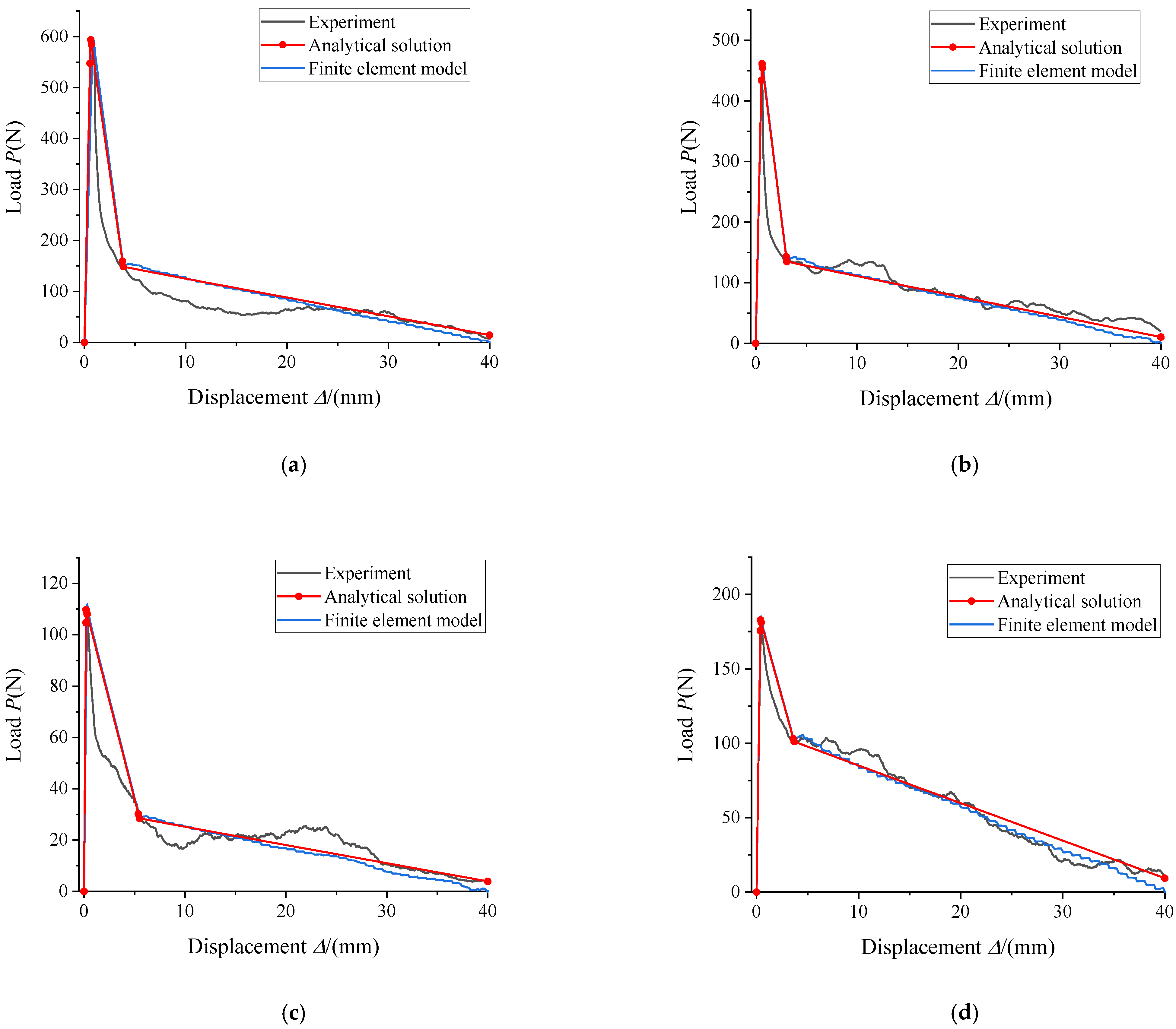
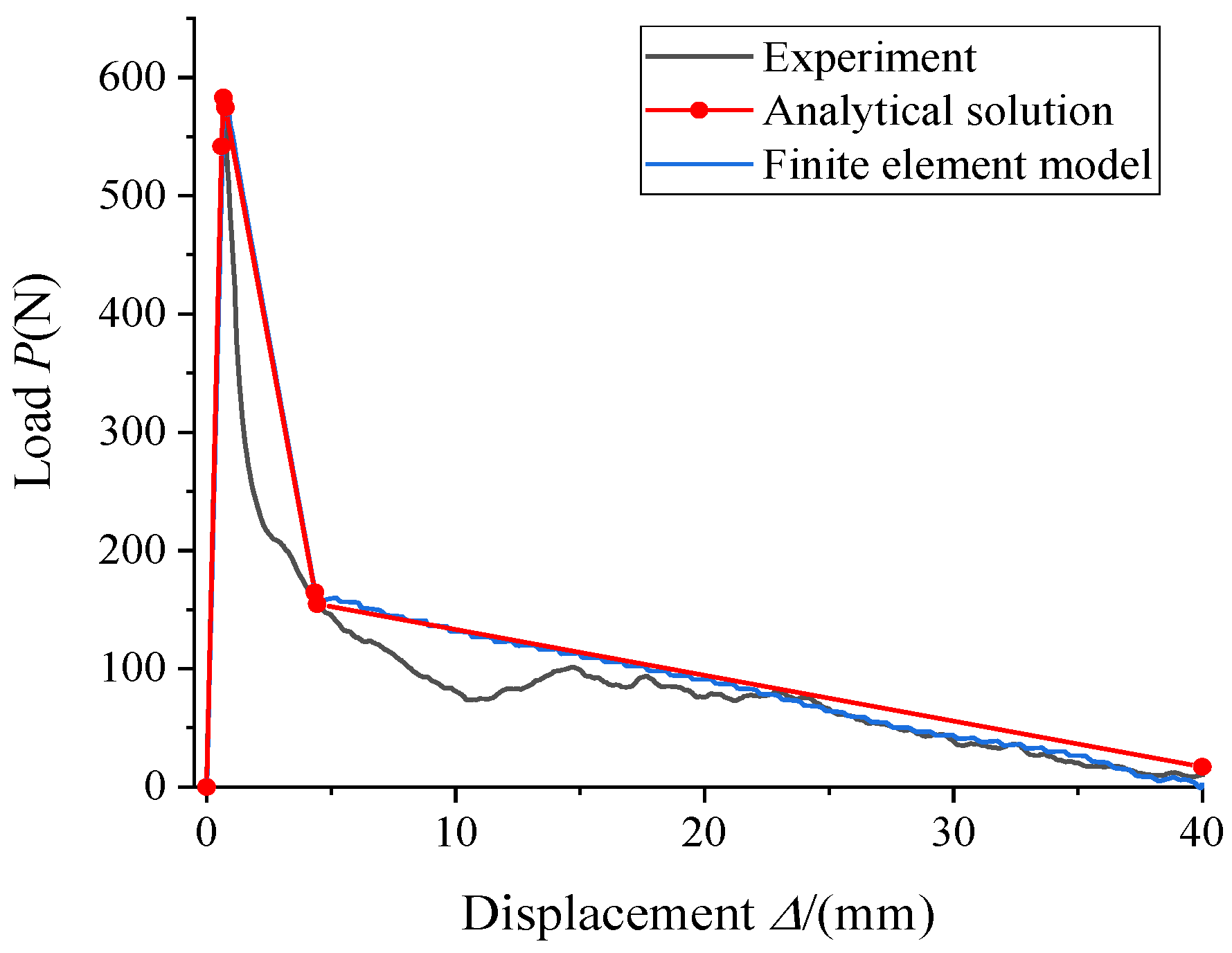
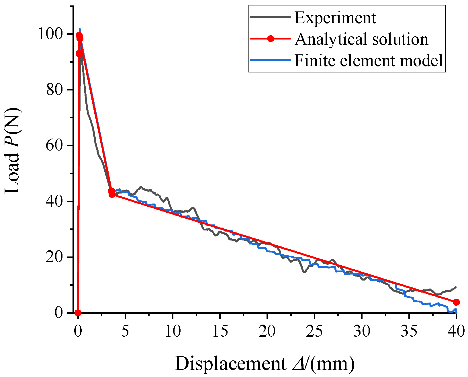
5.1. Modelling of the Single Fibre Pullout Tests

The FE mesh, boundary conditions, and geometry of the single fibre pullout tests are shown in Figure 20. The material properties are listed in

Table 3. Material parameters in FE simulations.

	E (GPa)	ν	ρ (kg/m3)	fc (MPa)	ft (MPa)	fy (MPa)	fb (MPa)	εb	rf (mm)	Lf (mm)
Mortar	20	0.20	2000	30	3
Fibre	200	0.33	7850			1400	1600	0.1	0.5	40
Interface	From test (Figure 19)			The curves in Figure 19 are used for the cohesive elements.

. The elemental size is 1 mm along the fibre, and, therefore, there are 40 fibre elements and 40 cohesive interface elements, respectively. Note that the slip distance or embedment length of the cohesive elements, ordered from the loaded end to the embedment end, is set as (L − δ₁)/40, 2 (L − δ₁)/40, 3 (L − δ₁)/40, …, 40(L − δ₁)/40, respectively. The simulated pullout load–displacement curves are shown in Figure 21, Figure 22, Figure 23 and Figure 24, with excellent agreement with the analytical solutions and the experimental data for all the ten groups of tests. In particular, the analytical solutions are accurately reproduced by the FE simulations, indicating the effectiveness of FE modelling approach. The slight discrepancies in the last stage may be caused by the damage plasticity of the mortar which is not considered in the analytical solutions but considered in the FE simulations.

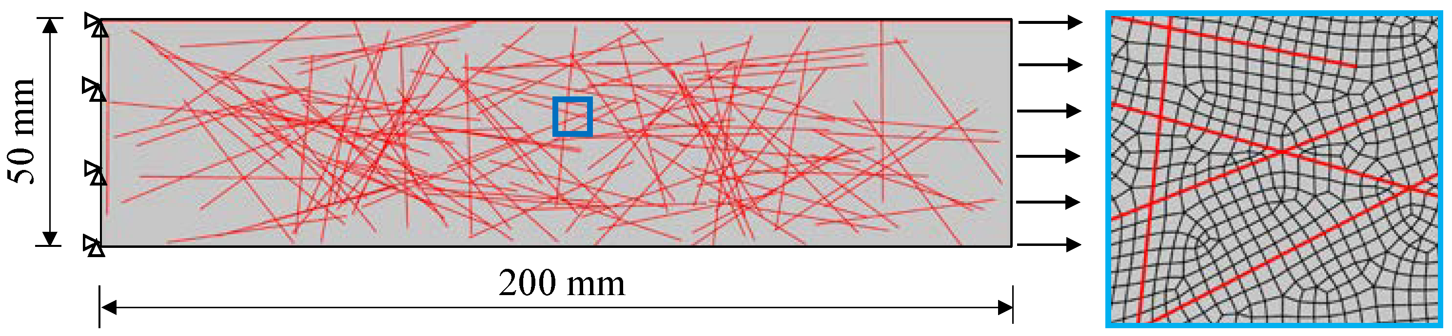
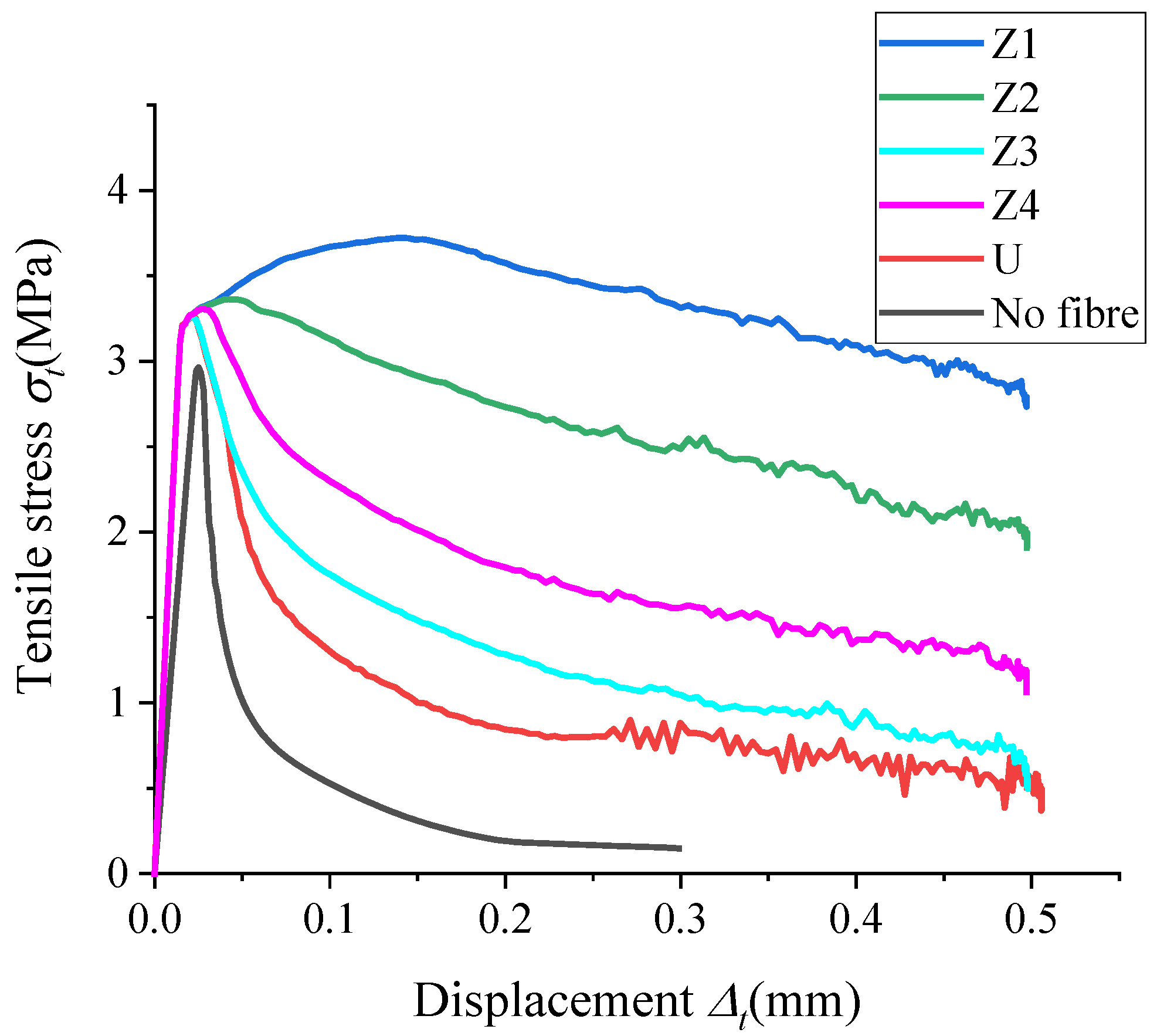
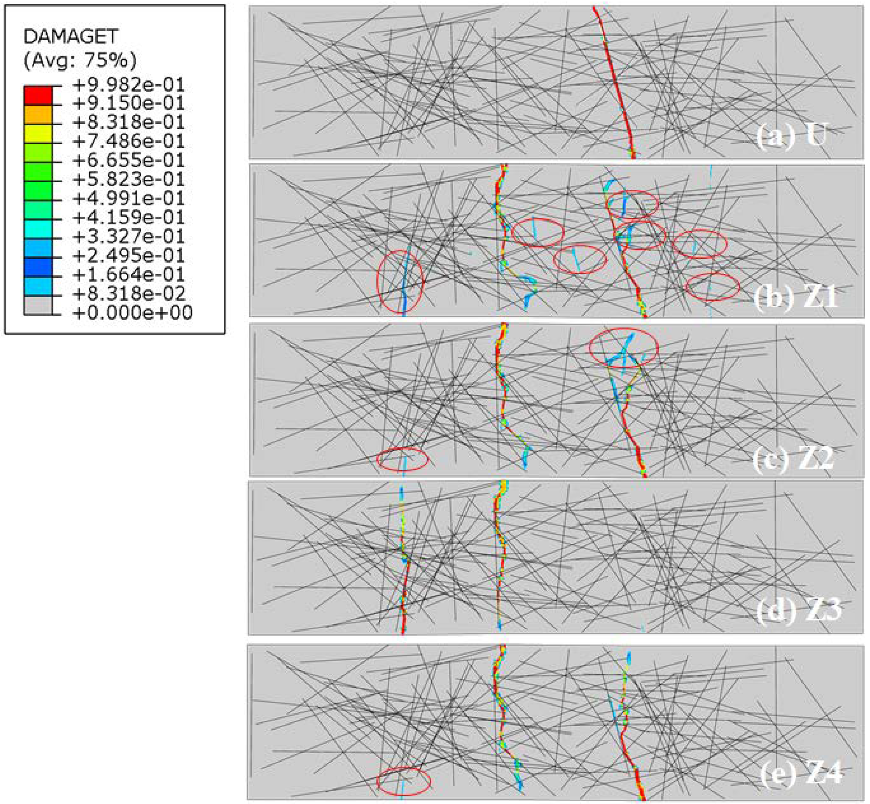
5.2. Direct Tensile Tests of SFRC Plates with Random Fibres

Figure 25 shows the geometry, boundary conditions, and a typical FE mesh used for an assumed SFRC plate with random fibres under uniaxial tension. The mean elemental size is 0.4 mm. Five mesoscale FE models with untreated fibres and those treated with four types of silane coatings (Z1–Z4), respectively, are simulated. The same material parameters listed in Table 3 and the same distribution of fibres are used for comparison. Figure 26 shows the final crack patterns. It can be seen that the model U has only one main crack, whereas the Z1–Z4 models have two main cracks. In addition, there are more secondary cracks in the models Z1 and Z2 than the others. This is due to the higher bonding properties of interfacial cohesive elements in Z1 and Z2 than the others, which have higher constraints in the mortar and, thus, more cracks to dissipate energy. This is also reflected in the simulated cross-sectional average stress-displacement curves, as shown in Figure 27. All of the models with silane coated fibres show improvement on the load-carrying capacities in terms of both structural strength and ductility (i.e., the area or energy consumption under the curve). In particular, the model Z1 exhibits the most significant strain-hardening effect after the first crack appears with the highest ductility, followed by Z2 and Z4 models. This is again consistent with the used bond-slip relations as shown in Figure 19 for different silane treated fibres. These results demonstrate that the technique of silane coating of fibres can not only enhance structural performance, but also can change the structural failure mode from brittle to ductile.

It is noteworthy that the simulated failure patterns in Figure 26 can be directly validated only when real internal distributions of fibres are available and taken into account in the FE models. This can be realized by advanced techniques such as in-situ X-ray computed tomography scanning under progressive loadings and high-fidelity image-based FE simulations [47,48].

6. Conclusions

This study has carried out a systematic investigation of the effects of nine types of silane coatings on the steel fibre–mortar interfacial bond properties, combining pullout tests, analytical solutions, and mesoscale FE simulations. The following main conclusions can be drawn:

(1) The 30 single fibre pullout tests show that coating steel fibres by nine types of silane solutions leads to 11–575% increase on the bonding strength at peak load, 0.1–789% increase on the chemical bond strength, 20–279% increase on the residual frictional strength, and 2–248% increase on the pullout energy. Overall, the pure silane solution Z6011 is the most effective one, followed by Z6020 and Z6040, whereas the Z6030 solution is not effective. The addition of H₂ZrF₆ further enhances the bond strength but the addition of Zr(NO₃)₄ has adverse effects. The Z6020, Z6011, and Z6020 solutions mixed with H₂ZrF₆ mainly improve the chemical bond strength, while the Z6030 and Z6040 ones mainly improve the residual frictional strength.

(2) Based on a simple tri-linear interfacial bond-slip model, closed-form analytical solutions of the load–displacement curves and the distributions of fibre strength, interfacial stresses and slips along the embedment length, are derived for five stages of the whole pullout process for relatively short embedment length of fibres. The four parameters δ₁, τ_f, δ_f, and τ_r (or k) in the bond-slip model are calibrated against the pullout test data for untreated steel fibres and those with the nine types of silane coatings.

(3) The calibrated bond-slip models are then successfully used as interfacial constitutive laws to simulate the single fibre pullout tests and more complicated damage and fracture behaviour of multi-fibre tensile models, using a discrete-continuum coupled mesoscale finite element approach. The numerical simulations demonstrate that the technique of silane coating of fibres can not only enhance the structural performances in terms of higher strength and ductility, but also can change the structural failure mode from brittle to ductile.

(4) The developed approach of combining single fibre/bar pullout tests, analytical solutions and numerical modelling, provides a systematic and feasible way to investigate the effects of interfacial properties between fibres/bars and mortar/concrete, which are difficult to measure directly from pullout tests (e.g., using conventional strain gauges), on the complicated deformation and failure behaviour of SFRC, UHPFRC, and RC structural members.

(5) Experimental and numerical studies of silane-coated SFRC structural members need to be carried out under complicated loading conditions before this technique can be confidently used in engineering practice. Thinner fibres should also be studied to investigate potential scale effects of the fibre diameter.

References

1. Song, P.S.; Hwang, S. Mechanical properties of high-strength steel fiber-reinforced concrete. Constr. Build. Mater. 2004, 18, 669–673. [Google Scholar] [CrossRef]
2. Redon, C.; Li, V.; Wu, C.; Hoshiro, H.; Saito, T.; Ogawa, A. Measuring and Modifying Interface Properties of PVA Fibers in ECC Matrix. J. Mater. Civ. Eng. 2001, 13, 399–406. [Google Scholar] [CrossRef]
3. Vrijdaghs, R.; Prisco, M.D.; Vandewalle, L. Short-term and creep pull-out behavior of polypropylene macrofibers at varying embedded lengths and angles from a concrete matrix. Constr. Build. Mater. 2017, 147, 858–864. [Google Scholar] [CrossRef]
4. Lee, A.T.; Michel, M.; Ferrier, E.; Benmokrane, B. Influence of curing conditions on mechanical behaviour of glued joints of carbon fiber-reinforced polymer composite/concrete. Constr. Build. Mater. 2019, 227, 116385. [Google Scholar] [CrossRef]
5. Cheng, C.; He, J.; Zhang, J.; Yang, Y. Study on the time-dependent mechanical properties of glass fiber reinforced cement (GRC) with fly ash or slag. Constr. Build. Mater. 2019, 217, 128–136. [Google Scholar] [CrossRef]
6. Dvorkin, L.; Dvorkin, O. Basics of Concrete Science; Stroi-Beton: St-Petersburg, Russia, 2006; ISBN 590319702-7. [Google Scholar]
7. Liew, K.; Akbar, A. The recent progress of recycled steel fiber reinforced concrete. Constr. Build. Mater. 2020, 232, 117232. [Google Scholar] [CrossRef]
8. Nataraja, M.C.; Dhang, N.; Gupta, A.P. Toughness characterization of steel fiber-reinforced concrete by JSCE approach. Cem. Concr. Res. 2000, 30, 593–597. [Google Scholar] [CrossRef]
9. Zhang, J.; Stang, H.; Li, V. Experimental Study on Crack Bridging in FRC under Uniaxial Fatigue Tension. J. Mater. Civ. Eng. 2000, 12, 66–73. [Google Scholar] [CrossRef]
10. Singh, S.P.; Kaushik, S.K. Fatigue strength of steel fiber reinforced concrete in flexure. Cem. Concr. Compos. 2003, 25, 779–786. [Google Scholar] [CrossRef]
11. Li, V.C.; Stang, H.; Krenchel, H. Micromechanics of crack bridging in fiber-reinforced concrete. Mater. Struct. 1993, 26, 486–494. [Google Scholar] [CrossRef]
12. Li, V.C.; Stang, H. Interface property characterization and strengthening mechanisms in fiber reinforced cement based composites. Adv. Cem. Based Mater. 1997, 6, 1–20. [Google Scholar] [CrossRef]
13. Soetens, T.; Gysel, A.V.; Matthys, S.; Taerwe, L. A semi-analytical model to predict the pull-out behaviour of inclined hooked-end steel fibers. Constr. Build. Mater. 2013, 43, 253–265. [Google Scholar] [CrossRef]
14. Deng, F.; Ding, X.; Chi, Y.; Xu, L.; Wang, L. The pull-out behavior of straight and hooked-end steel fiber from hybrid fiber reinforced cementitious composite: Experimental study and analytical modelling. Compos. Struct. 2018, 206, 693–712. [Google Scholar] [CrossRef]
15. Khabaz, A. Performance evaluation of corrugated steel fiber in cementitious matrix. Constr. Build. Mater. 2016, 128, 373–383. [Google Scholar] [CrossRef]
16. Ye, J.; Liu, G. Pullout Response of Ultra-High-Performance Concrete with Twisted Steel Fibers. Appl. Sci. 2019, 9, 658. [Google Scholar] [CrossRef] [Green Version]
17. Won, J.P.; Lee, J.H.; Lee, S.J. Predicting pull-out behaviour based on the bond mechanism of arch-type steel fiber in cementitious composite. Compos. Struct. 2015, 134, 633–644. [Google Scholar] [CrossRef]
18. Yoo, D.-Y.; Chun, B.; Kim, J.-J. Bond performance of abraded arch-type steel fibers in ultra-high-performance concrete. Cem. Concr. Compos. 2020, 109, 103538. [Google Scholar] [CrossRef]
19. Hao, Y.; Hao, H. Pull-out behaviour of spiral-shaped steel fibers from normal-strength concrete matrix. Constr. Build. Mater. 2017, 139, 34–44. [Google Scholar] [CrossRef]
20. He, Q.; Liu, C.; Yu, X. Improving steel fiber reinforced concrete pull-out strength with nanoscale iron oxide coating. Constr. Build. Mater. 2015, 79, 311–317. [Google Scholar] [CrossRef]
21. Pi, Z.; Xiao, H.; Du, J.; Liu, M.; Li, H. Interfacial microstructure and bond strength of nano-SiO2-coated steel fibers in cement matrix. Cem. Concr. Compos. 2019, 103, 1–10. [Google Scholar] [CrossRef]
22. Miller, H.D.; Akbarnezhad, A.; Mesgari, S.; Foster, S.J. Performance of oxygen/argon plasma-treated steel fibers in cement mortar. Cem. Concr. Compos. 2019, 97, 24–32. [Google Scholar] [CrossRef]
23. Sun, M.; Wen, D.-J.; Wang, H.-W. Influence of corrosion on the interface between zinc phosphate steel fiber and cement. Mater. Corros. 2010, 63, 67–72. [Google Scholar] [CrossRef]
24. Soulioti, D.; Barkoula, N.-M.; Koutsianopoulos, F.; Charalambakis, N.; Matikas, T. The effect of fibre chemical treatment on the steel fibre/cementitious matrix interface. Constr. Build. Mater. 2013, 40, 77–83. [Google Scholar] [CrossRef]
25. Aggelis, D.; Soulioti, D.; Barkoula, N.; Paipetis, A.; Matikas, T. Influence of fiber chemical coating on the acoustic emission behavior of steel fiber reinforced concrete. Cem. Concr. Compos. 2012, 34, 62–67. [Google Scholar] [CrossRef]
26. Pax, G.M.; Bouchet, J.; Michaud, V.; Månson, J.-A.E. Tailoring of the practical adhesion between polyethylene and galvanised steel. J. Adhes. Sci. Technol. 2006, 20, 1255–1272. [Google Scholar] [CrossRef]
27. Alinejad, S.; Naderi, R.; Mahdavian, M. The effect of zinc cation on the anticorrosion behavior of an eco-friendly silane sol–gel coating applied on mild steel. Prog. Org. Coat. 2016, 101, 142–148. [Google Scholar] [CrossRef]
28. Chen, M.A.; Zhang, X.M.; Huang, R.; Lu, X.B. Mechanism of adhesion promotion between aluminium sheet and polypropylene with maleic anhydride-grafted polypropylene by gamma-aminopropyltriethoxy silane. Surf. Interface Anal. 2008, 40, 1209–1218. [Google Scholar] [CrossRef]
29. Underhill, R.S.; Fisher, G.C.; Farrell, S.P. Energy dispersive X-ray investigation of silane coupling agent modified nickel-manganese-gallium particle surfaces. Mater. Chem. Phys. 2012, 132, 253–257. [Google Scholar] [CrossRef]
30. Kong, X.-M.; Liu, H.; Lu, Z.-B.; Wang, D.-M. The influence of silanes on hydration and strength development of cementitious systems. Cem. Concr. Res. 2015, 67, 168–178. [Google Scholar] [CrossRef]
31. Felekoglu, B. A method for improving the early strength of pumice concrete blocks by using alky1 alkoxy silane (AAS). Constr. Build. Mater. 2012, 28, 305–310. [Google Scholar] [CrossRef]
32. Cao, J.; Chung, D. Improving the dispersion of steel fibers in cement mortar by the addition of silane. Cem. Concr. Res. 2001, 31, 309–311. [Google Scholar] [CrossRef]
33. Ma, Y.P. Study on Increasing of Interfacial Bond Strength between Cement Paste and Aggregate. J. Build. Mater. 1999, 2, 35–38. (In Chinese) [Google Scholar]
34. Benzerzour, M.; Sebaibi, N.; Abriak, N.E.; Binetruy, C. Waste fiber–cement matrix bond characteristics improved by using silane-treated fibers. Constr. Build. Mater. 2012, 37, 1–6. [Google Scholar] [CrossRef] [Green Version]
35. Sebaibi, N.; Benzerzour, M.; Abriak, N.E.; Binetruy, C. Mechanical properties of concrete-reinforced fibers and powders with crushed thermoset composites: The influence of fiber/matrix interaction. Constr. Build. Mater. 2012, 29, 332–338. [Google Scholar] [CrossRef]
36. Callens, M.G.; Gorbatikh, L.; Bertels, E.; Goderis, B.; Smet, M.; Verpoest, I. Tensile behaviour of stainless steel fiber/epoxy composites with modified adhesion. Compos. Part A Appl. Sci. Manuf. 2015, 69, 208–218. [Google Scholar] [CrossRef]
37. Liu, T.; Wei, H.; Zhou, A.; Zou, D.; Jian, H. Multiscale investigation on tensile properties of ultra-high performance concrete with silane coupling agent modified steel fibers. Cem. Concr. Compos. 2020, 111, 103638. [Google Scholar] [CrossRef]
38. Casagrande, C.A.; Cavalaro, S.H.P.; Repette, W.L. Ultra-high performance fiber-reinforced cementitious composite with steel microfibers functionalized with silane. Constr. Build. Mater. 2018, 178, 495–506. [Google Scholar] [CrossRef] [Green Version]
39. Wang, S.H.; Zhao, S.L.; Yang, S.Y.; Sun, B.; Shan, F.J. Preparation and performance of fluorozirconate-silane composite conversion film on cold-rolled steel surface. Electroplat. Finish. 2012, 31, 39–42. (In Chinese) [Google Scholar]
40. Ministry of Housing and Urban-Rural Development of the People’s Republic of China. JGJ/T 70-2009: Standard for Test Method of Basic Properties of Construction Mortar; Industry Standards of the People’s Republic of China; Ministry of Housing and Urban-Rural Development of the People’s Republic of China: Beijing, China, 2009. (In Chinese) [Google Scholar]
41. Leung, C.K.Y.; Shapiro, N. Optimal Steel Fiber Strength for Reinforcement of Cementitious Materials. J. Mater. Civ. Eng. 1999, 11, 116–123. [Google Scholar] [CrossRef]
42. Arkles, B. Tailoring Surfaces with Silanes; Chemtech.: West Chester, PA, USA, 1977; Volume 7, pp. 766–778. [Google Scholar]
43. Ren, F.; Yang, Z.; Chen, J.-F.; Chen, W. An analytical analysis of the full-range behaviour of grouted rockbolts based on a tri-linear bond-slip model. Constr. Build. Mater. 2010, 24, 361–370. [Google Scholar] [CrossRef]
44. Zou, X.X.; Sneed, L.H.; D’Antino, T. Full range behavior of fber reinforced cementitious matrix (FRCM)-concrete joints using a trilinear bond-slip relationship. Compos. Struct. 2020, 239, 112024. [Google Scholar] [CrossRef]
45. Lubliner, J.; Oliver, J.; Oller, S.; Onate, E. A plastic-damage model for concrete. Int. J. Solids Struct. 1989, 25, 299–326. [Google Scholar] [CrossRef]
46. Zhang, H.; Huang, Y.J.; Yang, Z.J.; Xu, S.L.; Chen, X.W. A discrete-continuum coupled finite element modelling approach for fibre reinforced concrete. Cem. Concr. Res. 2018, 106, 130–143. [Google Scholar] [CrossRef]
47. Yang, Z.; Qsymah, A.; Peng, Y.; Margetts, L.; Sharma, R. 4D characterisation of damage and fracture mechanisms of ultra high performance fibre reinforced concrete by in-situ micro X-Ray computed tomography tests. Cem. Concr. Compos. 2020, 106, 103473. [Google Scholar] [CrossRef]
48. Zhang, X.; Yang, Z.; Pang, M.; Yao, Y.; Li, Q.M.; Marrow, T.J. Ex-situ micro X-ray computed tomography tests and image-based simulation of UHPFRC beams under bending. Cem. Concr. Compos. 2021, 123, 104216. [Google Scholar] [CrossRef]
Figure 1. A specimen for the pullout test: (a) A specimen in mould; (b) A specimen demoulded; (c) The sketch.
Buildings 11 00398 g001
Figure 2. The device for single fibre pullout tests.
Buildings 11 00398 g002
Figure 3. Pullout P-Δ curves: steel fibres treated by four silane-based coupling agents (group Z): (a) Z1: Z6011; (b) Z2: Z6020; (c) Z3: Z6030; (d) Z4: Z6040.
Buildings 11 00398 g003
Figure 4. Pullout P-Δ curves: steel fibres treated by four silane-based coupling agents and Zr(NO3)4 (group ZZ): (a) ZZ1: Z6011 + Zr(NO3)4; (b) ZZ2: Z6020 + Zr(NO3); (c) ZZ3: Z6030 + Zr(NO3)4; (d) ZZ4: Z6040 + Zr(NO3)4.
Buildings 11 00398 g004
Figure 5. Pullout P-Δ curves: steel fibres treated by Z6020 + H2ZrF6 (group ZH2).
Buildings 11 00398 g005
Figure 6. Pullout P-Δ curves: untreated steel fibres (group U).
Buildings 11 00398 g006
Figure 7. Pullout forces (Pe, Pmax, Ps).
Buildings 11 00398 g007
Figure 8. Bonding strengths (τmax = τc + τs).
Buildings 11 00398 g008
Figure 9. Pullout energy.
Buildings 11 00398 g009
Figure 10. Increases of interfacial bonding strengths and pullout energy due to silane coatings.
Buildings 11 00398 g010
Figure 11. SEM micrographs and EDS spectra of steel fibres before pullout tests: (a) A micrograph of group U; (b) A micrograph of group Z1; (c) A micrograph of group ZZ1; (d) EDS spectra of group U; (e) EDS spectra of group Z1; (f) EDS spectra of group ZZ1.
Buildings 11 00398 g011
Figure 12. SEM micrographs of the ITZs: (a) An untreated fibre; (b) A fibre treated with Z6011 (group Z1).
Buildings 11 00398 g012
Figure 13. The idealized model of single fibre pullout tests.
Buildings 11 00398 g013
Figure 14. The tri-linear bond-slip model.
Buildings 11 00398 g014
Figure 15. Evolution of interfacial stress distribution along a steel fibre: (a,b) Elastic stage; (c,d) elastic–softening stage; (e,f) softening stage; (g,h) softening–debonding stage; (i) frictional stage; I, II and III represent elastic, softening, and debonding stress state, respectively.
Buildings 11 00398 g015
Figure 16. Full-range analytical load–displacement curve of single fibre pullout with short embedment length (not up to the real scale).
Buildings 11 00398 g016
Figure 17. Area analysis of shear stress evolution for Pmax (Point B in Figure 16), (a): corresponds to Figure 15b; (b): corresponds to Figure 15c; (c) corresponds to Figure 15d.
Buildings 11 00398 g017
Figure 18. Function diagram for f1(a) and f2(a).
Buildings 11 00398 g018
Figure 19. Calibrated tri-linear bond-slip models for all pullout tests (all curves are flat for 10 mm ≤ δ ≤ 40 mm).
Buildings 11 00398 g019
Figure 20. The finite element model of single pullout tests.
Buildings 11 00398 g020
Figure 21. Load–displacement curves from the pullout tests, analytical solutions and FE simulations (group Z): (a) Z1: Z6011; (b) Z2: Z6020; (c) Z3: Z6030; (d) Z4: Z6040.
Buildings 11 00398 g021aBuildings 11 00398 g021b
Figure 22. Load–displacement curves from the pullout tests, analytical solutions and FE simulations (group ZZ): (a) ZZ1: Z6011 + Zr(NO3)4; (b) ZZ2: Z6020 + Zr(NO3)4; (c) ZZ3: Z6030 + Zr(NO3)4; (d) ZZ4: Z6040 + Zr(NO3)4.
Buildings 11 00398 g022
Figure 23. Load–displacement curves from the pullout tests, analytical solutions and FE simulations (group ZH).
Buildings 11 00398 g023
Figure 24. Load–displacement curves from the pullout tests, analytical solutions and FE simulations (group U).
Buildings 11 00398 g024
Figure 25. The FE model of SFRC with random fibres under tension.
Buildings 11 00398 g025
Figure 26. Failure patterns of SFRC samples with different coatings under uniaxial tension.
Buildings 11 00398 g026
Figure 27. Tensile stress-displacement curves of SFRC models with different silane-coated fibres of random distribution under uniaxial tension.
Buildings 11 00398 g027