
Evaluating the Effect of External Horizontal Fixed Shading Devices’ Geometry on Internal Air Temperature, Daylighting and Energy Demand in Hot Dry Climate. Case Study of Ghardaïa, Algeria


Abstract
:
1. Introduction
- The ratio between slats vertical distance and their width : Datta [6] studied three values of (1, 2 and 0.92). Ouahrani and Al Touma [15] found that, for south orientation, a slat separation-to-width ratio of less than one () saves between 27.6% and 35.0% of the space total energy demand, eliminates glare visual discomfort and reduces CO2 emissions.
- The spacing between the slats: Oliveira [16] conducted a study of shading devices with a spacing of 0.23 m and 0.26 m depending on latitude. Hammad [10] from the United Arab Emirates set the spacing at 0.3 m and Alzoubi [20] from Jordan studied the case of spacing of 0.5 m; in both studies, the ratio s/l was equal to one, i.e., the vertical shading angle was 45°. In the United Kingdom, Freewan [13] fixed the ratio to the same value and spacing between the slats was fixed at 0.05 m.
- The tilted angle: In a previous study [1], the effect of three tilted angles (60°, 90° and 120°) on luminous and thermal conditions within spaces in hot climates was investigated. Hammad [10] and Alzoubi [20] both show that the total annual energy consumption and lighting level changes in correlation with the tilted angle of slats. Al Touma and Ouahrani [9] studied the impact of two tilted angles (45° and 90°) for north and south orientations. It was found that a tilted angle of 45° reduces energy demand by 7.7% and 18.6% for south and north-oriented offices, respectively; however, a tilted angle of 90° leads to 9.1% and 20.6% energy savings.
- Freewan [7] also carried out a comparative study on different types of shading devices (vertical fins, diagonal fins and an egg crate) where he varied several parameters: width of fins, spacing and tilted angle. Ossen et al. [8] studied the impact of solar shading geometry on building energy use in a hot humid climate.
2. Methodology
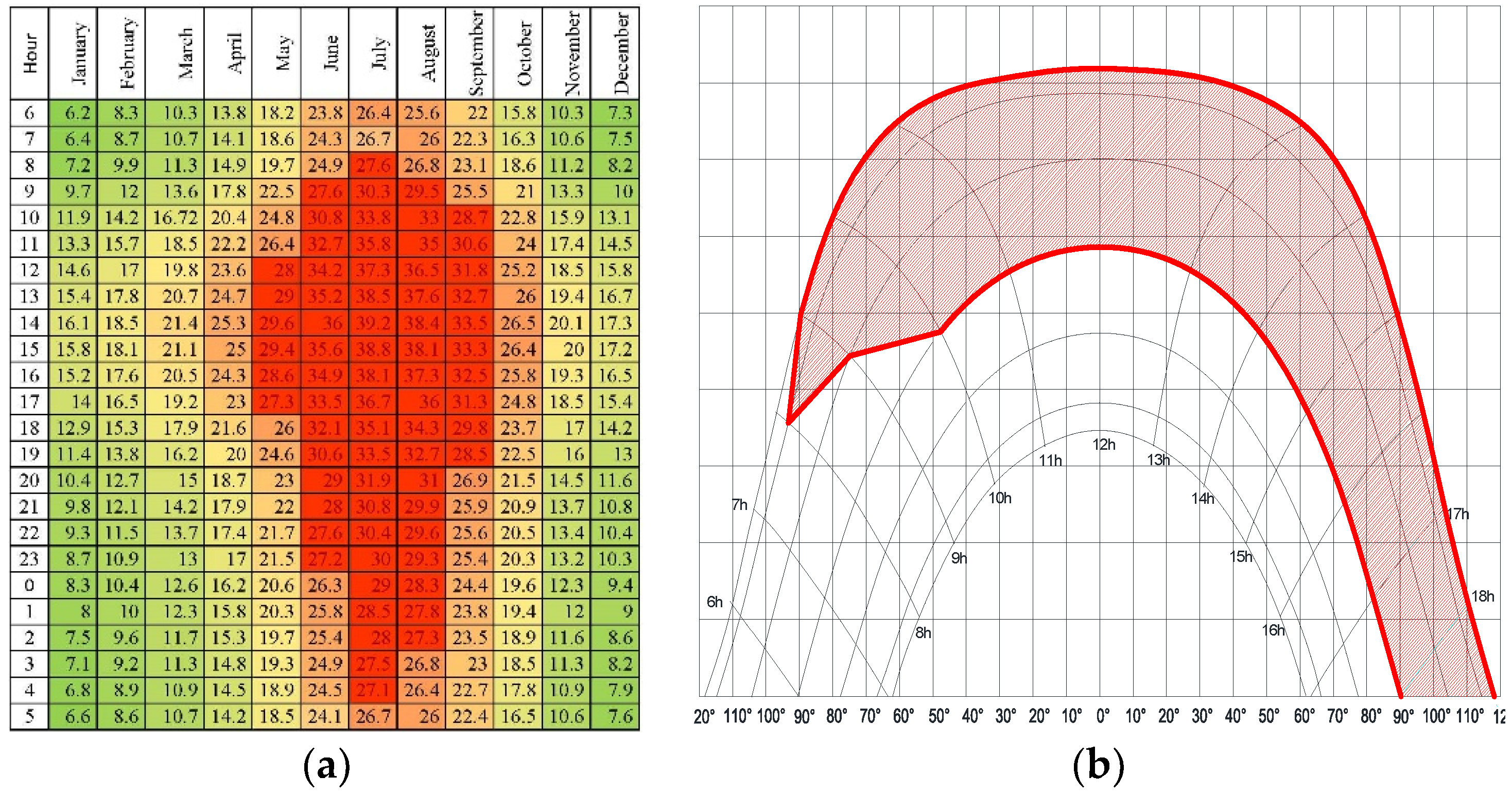
2.1. Study Area
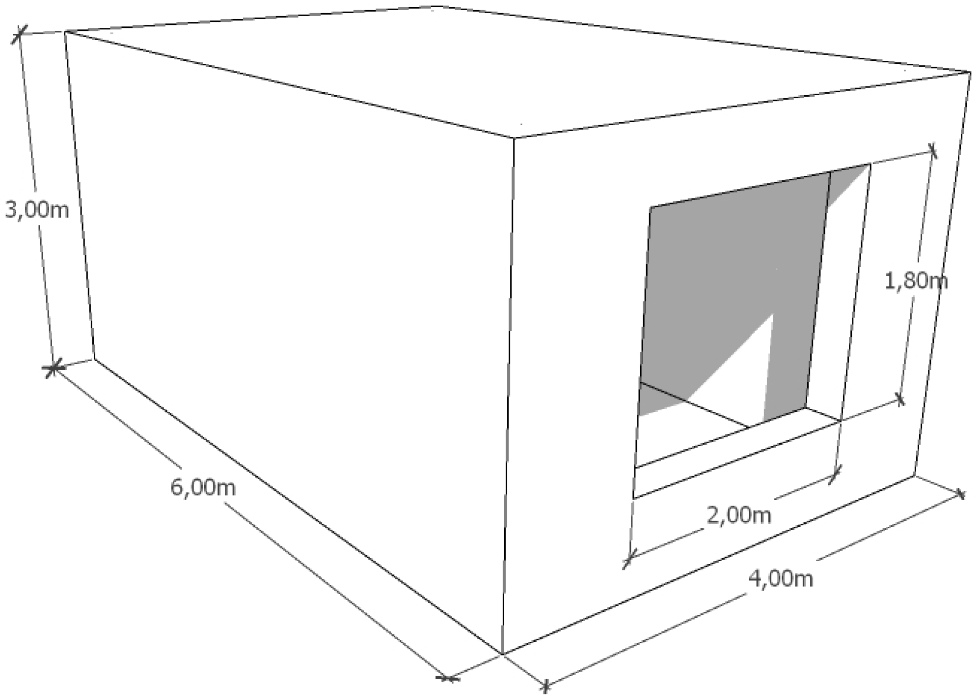
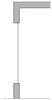
2.2. Case Study Description
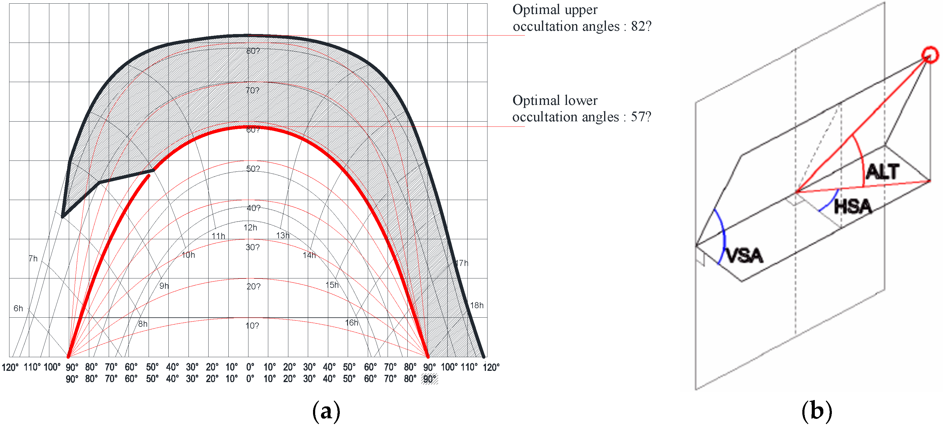
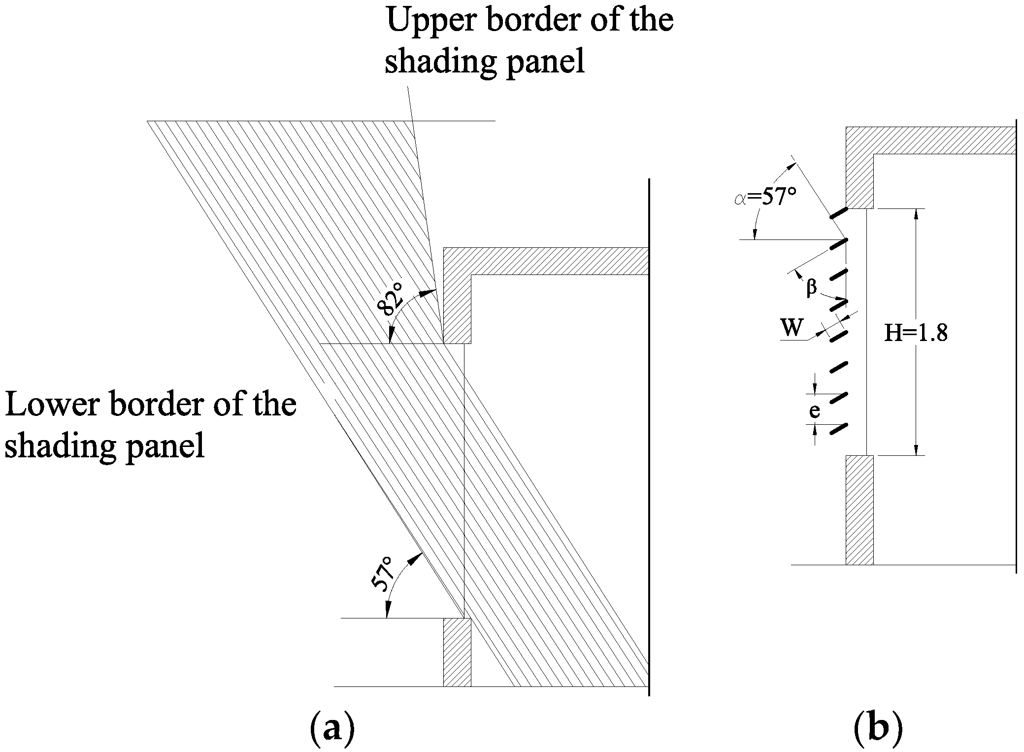
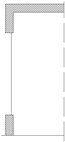
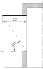
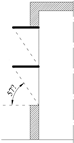
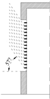
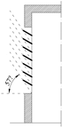
2.3. Sizing of Shading Devices and Geometries
- ALT: Altitude angle.
- VSA: Vertical shading angle.
- HSA: Horizontal shading angle.
- AZ: Azimuth.
- θ: Facade orientation.
- W: Slats width (m).
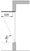
- α: Optimal lower vertical shading angle VSA = 57°.
- β: Tilted angle of the slats.
- e: Spacing between slats (m) = H/slats number.
- H: High of window (m) = 1.80.
- Vertical distance between slats “e”: H, H/2, H/4, H/8 and H/16;
- Slats tilted angles: 90° (horizontal), 60° and 120°; for this group of cases “e” was fixed to H/8. Additionally, installations of slats: vertical installation and horizontal installation with two tilted angles of slat (45° and 135°).
- A: Slats installation; V vertical, H horizontal.
- XX: Spacing between slats; 1-H, 2-H/2, 4-H/4, 8-H/8 and 16-H/16.
- YY: Tilted angle; 60–60°, 90–90°, 120–120°.
2.4. Simulation Tools and Conditions
2.4.1. Thermal Analysis
2.4.2. Daylighting Analysis
- Static daylight metrics, measured at a single point in time, using RADIANCE 2.0 to calculate illuminance level and DAYSIM 3.1 to calculate Daylight Factor (DF).
- Additionally, annual dynamic daylighting metrics using DAYSIM 3.1 to calculate daylight autonomy (DA), spatial daylight autonomy (sDA500lx,50%) and uniformity daylight factor (UDF).
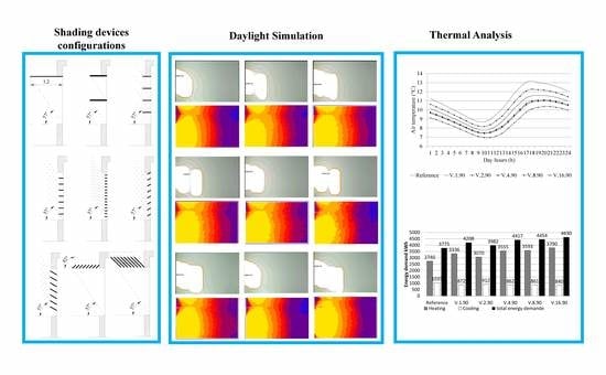
3. Results
3.1. Daylight Simulation
3.1.1. Spacing between Slats
3.1.2. Tilted Angle of the Slats
3.1.3. Slats Installation
3.2. Thermal Analysis
3.2.1. Air Temperature
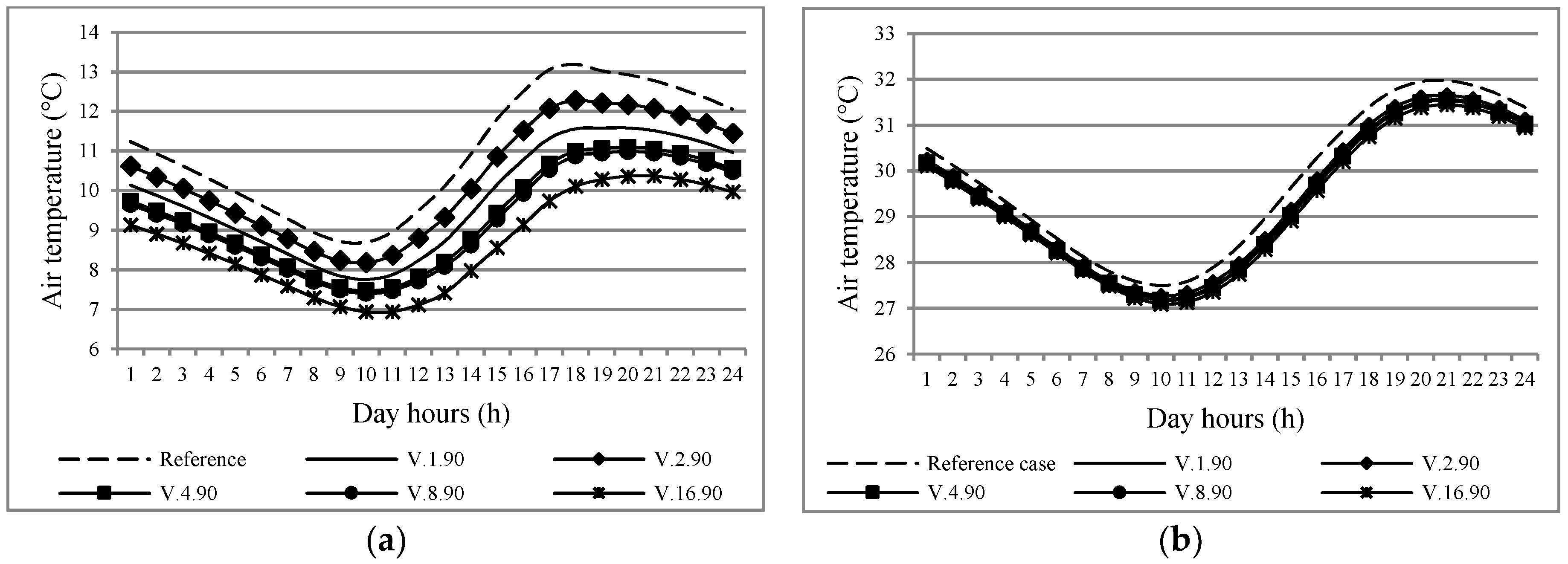
Spacing between Slats
- In January, in the afternoon the air temperature was reduced by up to 1 °C for the “V.2.90” case, 1.8 °C for the “V.1.90” case, 2.3 °C for both cases “V.4.90” and “V.8.90” and 3 °C for the “V.16.90” case. In the morning, the difference was less important; it was about 0.5 °C for case “V.2.90”, 0.9 °C for case “V.1.90”, 0.3 °C for both cases “V.4.90” and “V.8.90” and 1.7 °C for case “V.16.90”.
- However, in July, the difference of air temperature did not exceed 0.6 °C for all cases. Cases with different spacing between slats presented a similar behavior; they reduced the air temperature by approximately the same rate.
Tilted Angle of the Slats
- In January, the use of shading devices considerably reduced the indoor air temperature according to the reference case; we recorded a difference of 2.8 °C, 2.3 °C and 1.2 °C for cases “V.8.60”, “V.8.90” and “V.8.120”, respectively.
- However, the three cases presented almost the same air temperatures in July, with a difference of 0.5 °C compared to the reference case.
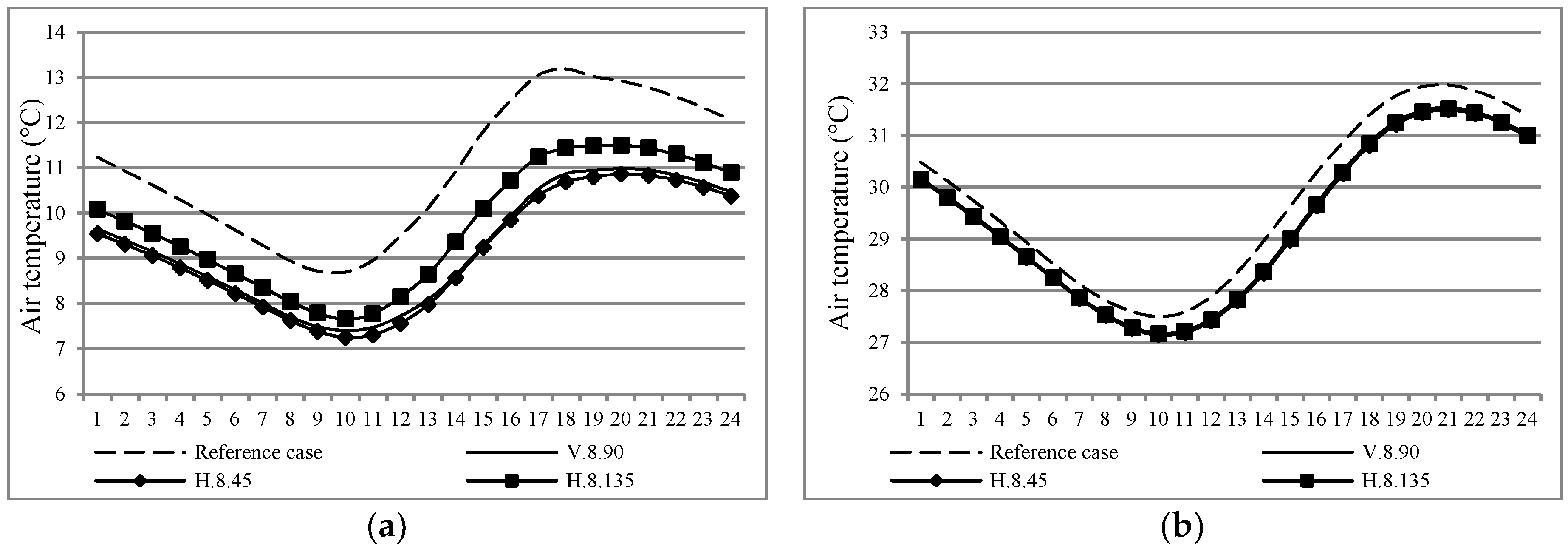
Slats Installation
- In January, in the afternoon the air temperature was reduced by up to 1.7 °C for case “H.8.135” and 2.5 °C for both cases “H.8.45” and “V.8.90”. In the morning, these differences were less important; they were about 1 °C for case “H.8.135” and 1.5 °C for cases “H.8.45” and V.8.90”.
- In July, the three cases presented a similar behavior, and the difference in air temperature did not exceed 0.4 °C.
3.2.2. Cooling and Heating Energy Demand
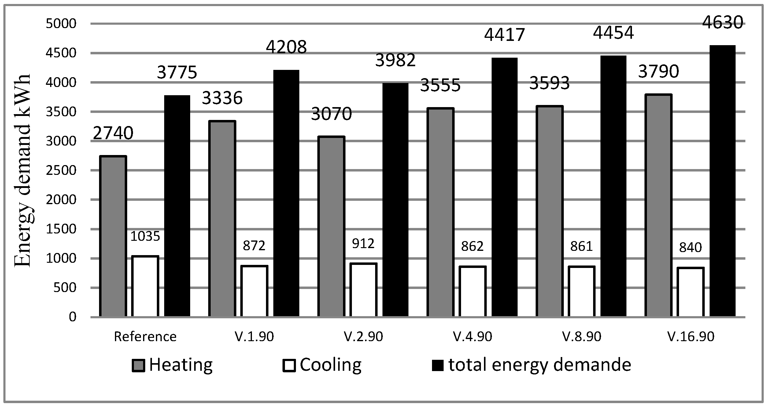
Vertical Distance between Slats
- The cooling energy saving results for cases “V.1.90”, “V.2.90”, “V.4.90”, “V.8.90” and “V.16.90” reached 16%, 12%, 17%, 17% and 19%, respectively. However, the use of shading devices with different slat spacing produced a negative effect on the heating energy demand, where energy saving was negative in all cases.
- The energy use for heating, compared to the reference case, increased by 21%, 12%, 29%, 31% and 38% for cases “V.1.90”, “V.2.90”, “V.4.90” and “V.8.90”, respectively.
- The total energy demand increased for all cases compared to the reference case, i.e., without shading devices. Case “V.2.90” presented the lowest value; it increased the total energy demand by only 5.5%. However, case “V.16.90” recorded the highest value; it increased the total energy demand by 22.6%. Cases “V.1.90”, “V.4.90” and “V.8.90” were, respectively, up by 11.5%, 17% and 18%.
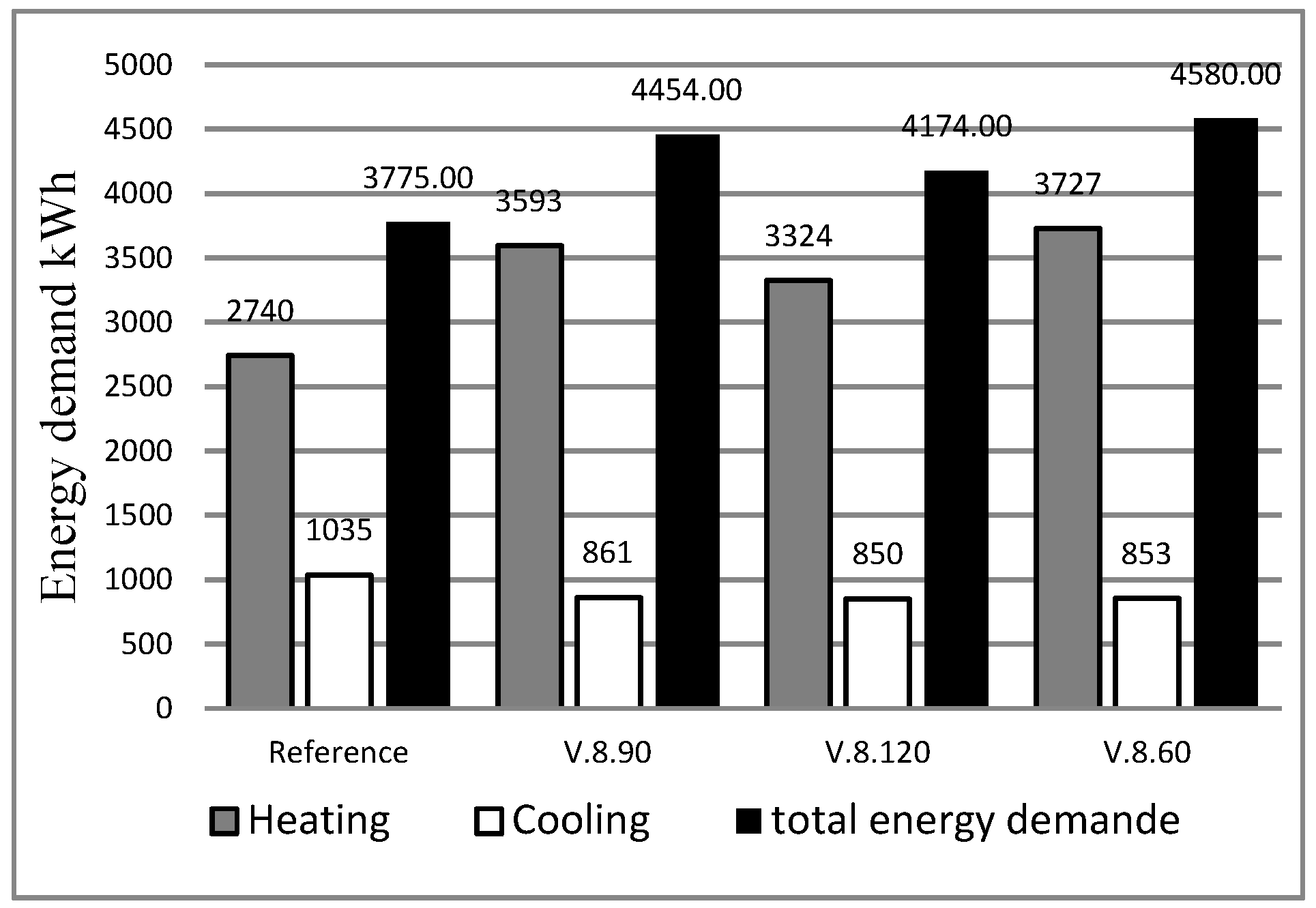
Tilted Angle of the Slats
- The cooling energy saving was about 17% compared to the reference case. However, the use of shading devices with different tilted angles increased the heating energy demand that was reduced by 36%, 31% and 21% corresponding to cases “V.8.60”, “V.8.90” and “V.8.120”, respectively.
- We note that the heating energy demand increased by reducing the slat tilted angle. This was mainly due to the direct solar radiation that decreased by the reducing slat tilted angle.
- The total energy demand also increased by using shading devices with different tilted angles; we recorded an increase of about 10,5%, 18% and 21% corresponding to cases “V.8.120”, “V.8.90” and “V.8.60”, respectively.
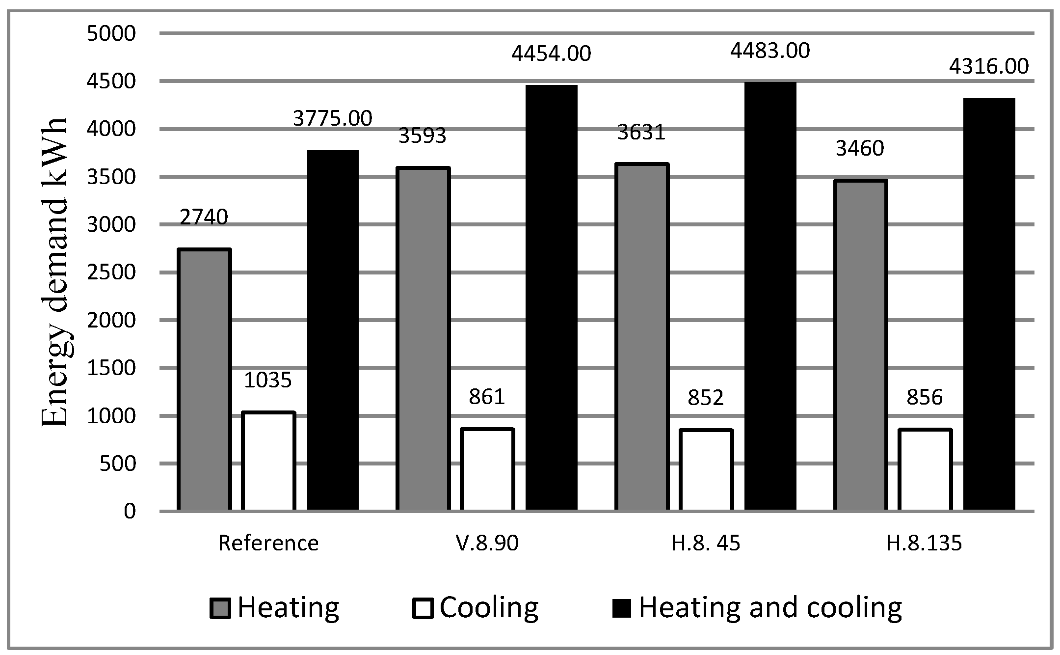
Slats Installation
- All cases decreased the cooling energy demand compared to the reference case. We note that the two cases with a horizontal installation, i.e., cases “H.8.45” and “H.8.135”, recorded a cooling energy demand less than the case with a vertical installation, although the difference between the three cases was insignificant, since the energy saving was about 17% compared to the reference case.
- Nevertheless, the three cases increased the heating energy demand. The “H.8.135” case presented the lowest value that was increased by 26% compared to the reference case. Cases “V.8.90” and “H.8.45” increased the heating energy demand by 31% and 32% similarly.
- The total energy demand increased in all cases; case “H.8.135” recorded the lowest value that was up by 14% compared to the reference case. The other two cases almost recorded the same total energy demand. The increase was about 18% for case “V.8.90” and 19% for case “H.8.45”.
4. Discussion
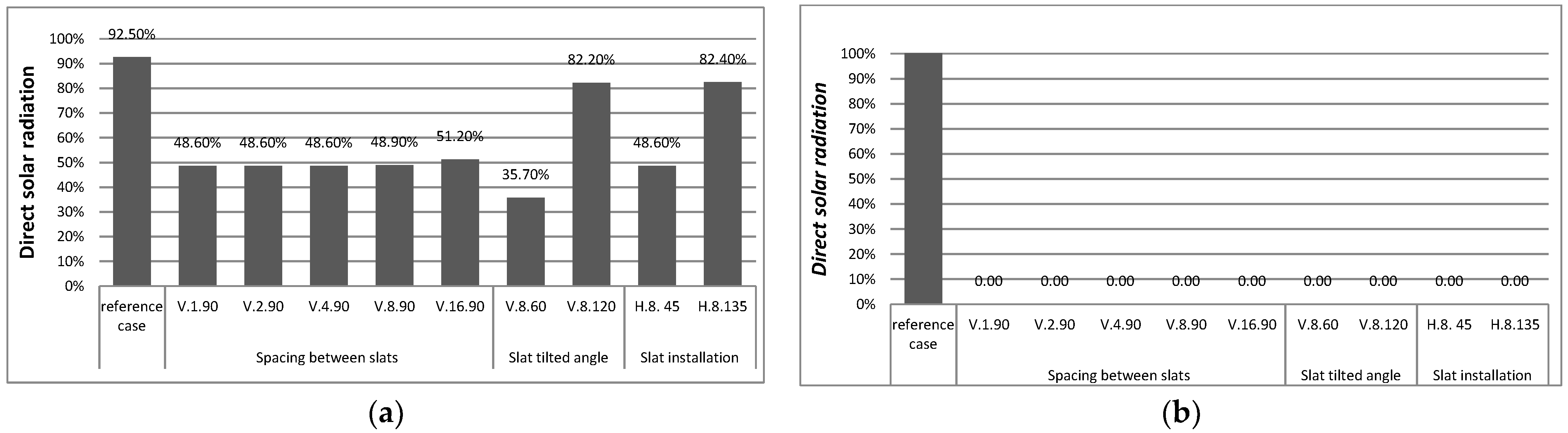
- The amount of direct solar radiation: it is the ratio between the sunny window area and the window area (Figure 12)
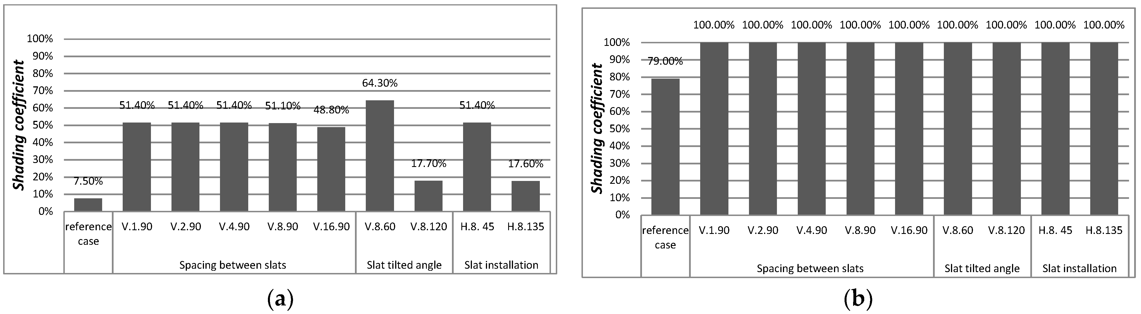
- Shading coefficient: it is the ratio between the shading window area and the window area. It is equal to 100- Direct solar radiation (Figure 13)
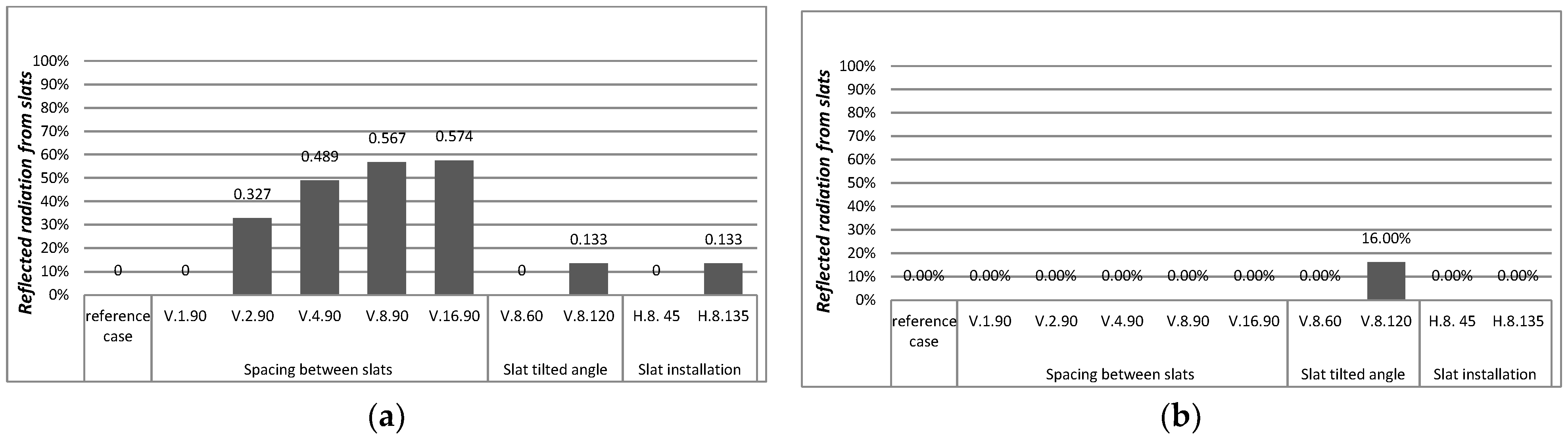
- Reflected radiation from slats: it is the ratio between the amount of solar radiation reflected by slats arriving to the window (m2) and the window area (Figure 14)
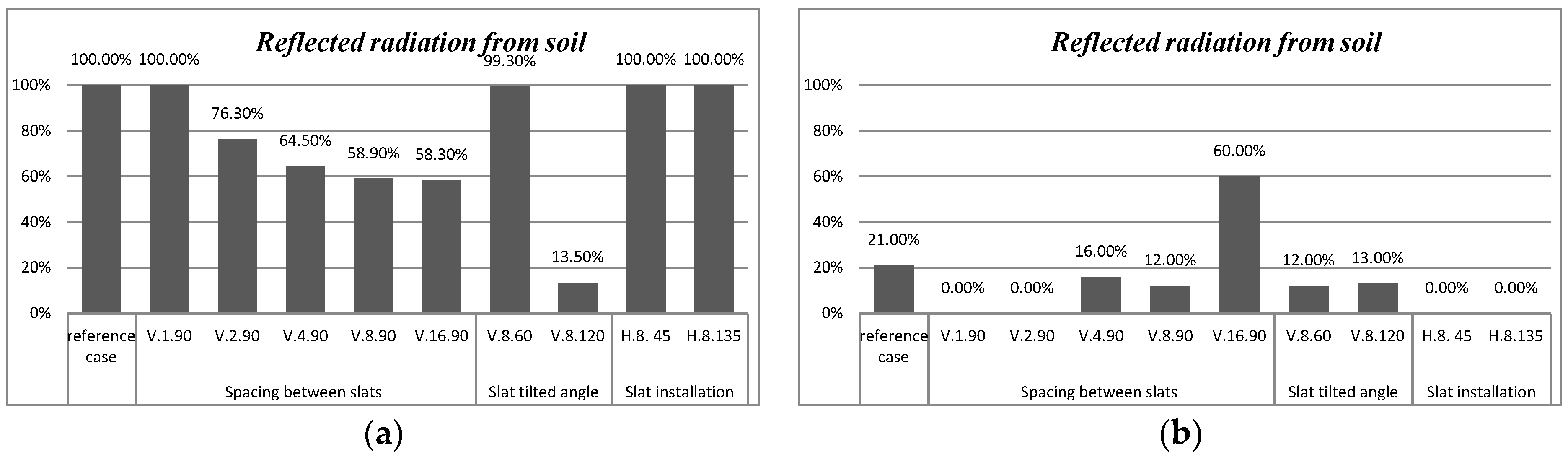
- Reflected radiation from soil: it is the ratio between the amount of solar radiation reflected by soil arriving to the window (m2) and the window area (Figure 15)
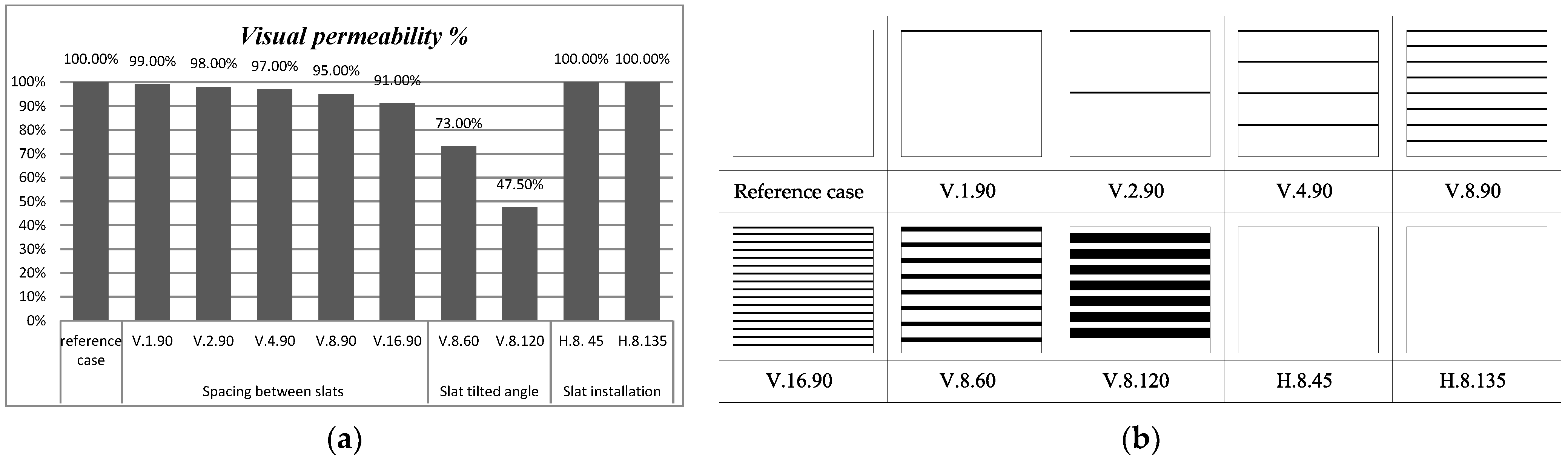
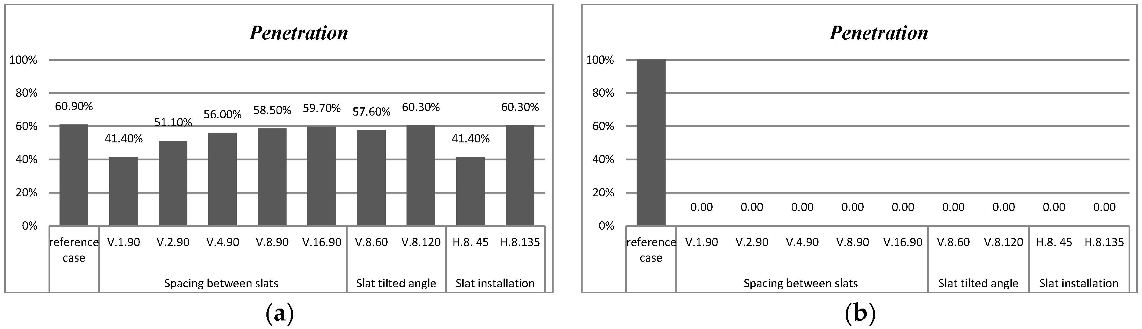
- Penetration of solar radiation, defined by the ratio of distance, measured from the facade, reached by the direct solar radiation to the space depth (Figure 16). And the visual permeability that depends only on shading devices configuration i.e., spacing between slats, slat tilted angle and slat installation. It is the ratio between projected open area and window area. In other words, visual permeability is the difference between the window area and the projected shaded area (Figure 17).
5. Conclusions
Author Contributions
Funding
Acknowledgments
Conflicts of Interest
References
- Magri, S.; Ait Haddou, H.; Boussoualim, A. Luminous and thermal effect of slat angle solar protection in hot climates. In Proceedings of the International Conference on Environment and Renewable Energy, Vienna, Austria, 20–21 May 2015. [Google Scholar]
- Dubois, M.-C. Solar Shading and Building Energy Use, a Literature Review, Part 1; Lund University: Lund, Sweden, 1997. [Google Scholar]
- Datta, G. Effect of fixed horizontal louver shading devices on thermal perfomance of building by TRNSYS simulation. Renew. Energy 2001, 23, 497–507. [Google Scholar] [CrossRef]
- Tzempelikos, A.; Athienitis, A.; Zmeureanu, R. The impact of shading design and control on building cooling and lighting demand. Sol. Energy 2007, 81, 369–382. [Google Scholar] [CrossRef]
- Tzempelikos, A.; Bessoudo, M.; Athienitis, A.; Zmeureanu, R. Indoor thermal environ-mental conditions near glazed facades with shading devices—Part II: Thermal comfort simula-tion and impact of glazing and shading properties. Build. Environ. 2010, 45, 2517–2525. [Google Scholar] [CrossRef]
- Bessoudo, M.; Tzempelikos, A.; Athienitis, A.; Zmeureanu, R. Indoor thermal environmental conditions near glazed facades with shading devices—Part I: Experiments and building thermal model. Build. Environ. 2010, 45, 2506–2516. [Google Scholar] [CrossRef]
- Freewan, A.A. Impact of external shading devices on thermal and daylighting performance of offices in hot climate regions. Sol. Energy 2014, 102, 14–30. [Google Scholar] [CrossRef]
- Ossen, D.R.; Ahmad, M.H.; Madros, N.H. Impact of solar shading geometry on building energy use in hot humid climates with special reference to Malaysia. In Proceedings of the NSEB2005—SUS-TAINABLE SYMBIOSIS, National Seminar on Energy in Buildings, Shah Alam, Malaysia, 10–11 May 2005. [Google Scholar]
- Al Touma, A.; Ouahrani, D. Shading and day-lighting controls energy savings in offices with fully-Glazed façades in hot climates. Energy Build. 2017, 151, 263–274. [Google Scholar] [CrossRef]
- Hammad, F.; Abu-Hijleh, B. The energy savings potential of using dynamic external louvers in an office building. Energy Build. 2010, 42, 1888–1895. [Google Scholar] [CrossRef]
- Dubois, M.-C. Shading devices and daylight quality: An evaluation based on simple performance indicators. Light. Res. Technol. 2003, 35, 61–74. [Google Scholar] [CrossRef]
- Wong, N.H.; Djoko, A.I. Effect of external shading devices on daylighting penetration in residential buildings. Light. Res. Technol. 2004, 36, 317–333. [Google Scholar] [CrossRef]
- Freewan, A.A.; Shao, L.; Riffat, S. Interactions between louvers and ceiling geometry for maximum daylighting performance. Renew. Energy 2009, 34, 223–232. [Google Scholar] [CrossRef]
- Kim, G.; Lim, H.S.; Lim, T.S.; Schaefer, L. Comparative advantage of an exterior shading device in thermal performance for residential buildings. Energy Build. 2012, 46, 105–111. [Google Scholar] [CrossRef]
- Ouahrani, D.; Al Touma, A. Selection of slat separation-to-width ratio of brise-soleil shading considering energy savings, CO2 emissions and visual comfort—A case study in qatar author links open overlay panel. Energy Build. 2018, 165, 440–450. [Google Scholar] [CrossRef]
- Palmero-Marrero, A.I.; Oliveira, A.C. Effect of louver shading devices on building energy requirements. Appl. Energy 2014, 87, 2040–2049. [Google Scholar] [CrossRef]
- Cillari, G.; Fantozzi, F.; Franco, A. Passive Solar Solutions for Buildings: Criteria and Guidelines for a Synergistic Design. Appl. Sci. 2021, 11, 376. [Google Scholar] [CrossRef]
- Tzempelikos, A.; Roy, M. A Simulation Design Study for the Facade Renovation. In Proceedings of the Canadian Solar Buildings Conference 2004, Montreal, QC, USA, 20–24 August 2004. [Google Scholar]
- David, M.; Donn, M.; Garde, F.; Lenoir, A. Assessment of the thermal and visualefficiency of solar shades. Build. Environ. 2011, 46, 1489–1496. [Google Scholar] [CrossRef]
- Alzoubi, H.H.; Al-Zoubi, A.H. Assessment of building façade performance in terms of daylighting and the associated energy consumption in architectural spaces: Vertical and horizontal shading devices for southern exposure facades. Energy Conver. Manag. 2010, 51, 1592–1599. [Google Scholar] [CrossRef]
- Vera, S.; Uribe, D.; Bustamante, W.; Molina, G. Optimization of a fixed exterior complex fenestration system considering visual comfort and energy performance criteria. Build. Environ. 2016, 113, 163–174. [Google Scholar] [CrossRef]
- Kim, J.T.; Kim, G. Advanced External Shading Device to Maximize Visual and View Performance. Indoor Built Environ. 2010, 19, 65–72. [Google Scholar] [CrossRef]
- Nielsen, M.V.; Svendsen, S.; Jensen, L.B. Quantifying the potential of automated dynamic solar shading in office buildings through integrated simulations of energy and day-light. Sol. Energy 2011, 85, 757–768. [Google Scholar] [CrossRef]
- Settino, J.; Carpino, C.; Perrella, S.; Arcuri, N. Multi-Objective Analysis of a Fixed Solar Shading System in Different Climatic Areas. Energies 2020, 13, 3249. [Google Scholar] [CrossRef]
- Al-Tamimi, N.A.; Fadzil, S.F. The potential of shading devices for temperature reductionin high-rise residential buildings in the tropics. Procedia Eng. 2011, 273–282. [Google Scholar] [CrossRef] [Green Version]
- Bader, S. High-Performance Façades for Commercial Buildings; The University of Texas Austin: Austin, TX, USA, 2011. [Google Scholar]
- Szokolay, S.V. PLEA Notes: Solar Geometry; PLEA Passive and Low Energy Architecture International and University of Queensland: Brisbane, QLD, Australia, 1996. [Google Scholar]
- Kottek, M.; Grieser, J.; Beck, C.; Rudolf, B.; Rubel, F. World Map of the Köppen-Geiger climate classification updated. Meteorol. Z. 2006, 15, 259–263. [Google Scholar] [CrossRef]
- Djenane, M.; Farhi, A.; Benzerzour, M.; MUSY, M. Microclimatic behaviour of urban forms in hot dry regions. Towards a definition of adapted indicators. In Proceedings of the 25th Conference on Passive and Low Energy Architecture PLEA, Dublin, Ireland, 22–24 October 2008. [Google Scholar]
- Capderou, M. Atlas Solaire de L’algérie; Office des Publications Universitaires: Alger, Algeria, 1986. [Google Scholar]
- Matusiak, B. A design method for fixed outside solar shading device. In Proceedings of the PLEA2006 the 23rd Conference on Passive and Low Energy Architecture, Geneva Switzerland, 6–8 September 2006. [Google Scholar]
- Lawrence Berkeley National Laboratory. Desktop Radiance v.1.02 [ComputerSoftware]. Available online: http://radsite.lbl.gov/deskrad (accessed on 10 December 2019).
- Reinhart, C.F.; Walkenhorst, O. Validation of dynamic RADIANCE-based daylight simulations for a test office with external blinds. Energy Build. 2001, 33, 683–697. [Google Scholar] [CrossRef]
- British Standards Institution. Lighting for Buildings—Part 2: Code of Practice for Daylighting; BS 8206-2:2008; British Standards Institution: London, UK, 2008. [Google Scholar]
- Michael, A.; Gregoriou, S.; Kalogirou, S. Environmental assessment of an integrated adaptive system for the improvement of indoor visual comfort of existing buildings. Renew. Energy 2018, 115, 620–633. [Google Scholar] [CrossRef]
- Reinhart, C.; Mardaljevic, J.; Rogers, Z. Dynamic Daylight Performance Metrics for Sus-tainable Building Design. LEUKOS 2006, 3, 7–31. [Google Scholar] [CrossRef] [Green Version]
- Harberl, J.; Kota, S. Historical survey of daylighting calculations methods and their use in energy performance simulations. In Proceedings of the 9th International Conference for Enhanced Building Operations, Austin, TX, USA, 17–19 November 2009; pp. 1–9. [Google Scholar]
- Heschong, L.; Wymelenberg, V.; Andersen, M.; Digert, N.; Fernandes, L.; Keller, A.; Love-land, J.; McKay, H.; Mistrick, R.; Mosher, B. Approved Method: IES Spatial Daylight Autonomy (sDA) and Annual Sunlight Exposure (ASE); IES-Illuminating Engineering Society: New York, NY, USA, 2012. [Google Scholar]
- USGBC. Daylight. Retrieved 14 November 2020. Available online: https://www.usgbc.org/credits/healthcare/v4-draft/eqc-0 (accessed on 2 February 2021).
- Moon, P.; Spencer, D. Illumination from a nonuniform sky. Illum. Eng. 1942, 37, 707–726. [Google Scholar]
- Iversen, A.; Roy, N.; Hvass, M.; Jorgensen, M.; Christoffersen, J.; Osterhaus, W.; Johnsen, K. Daylighting Calculations in Practice; Aalborg University: Copenhagen, Denmark, 2013. [Google Scholar]


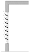
| Reference Case | V.1.90 | V.2.90 | V.4.90 | V.8.90 | |
|---|---|---|---|---|---|
 |  |  |  |  | |
| Installation | / | Vertical | Vertical | Vertical | Vertical |
| Slat spacing | / | H = 1.8 m | H/2 = 0.90 m | H/4 = 0.45 | H/8 = 0.22 m |
| Tilted angle | / | 90° | 90° | 90° | 90° |
| Width (m) | / | 1.2 | 0.6 | 0.3 | 0.15 |
| V.16.90 | V.8.60 | V.8.120 | H.8.45 | H.8.135 | |
 |  |  |  |  | |
| Installation | Vertical | Vertical | Vertical | Horizontal | Horizontal |
| Slat spacing | H/16 = 0.11 m | H/8 = 0.22 m | H/8 = 0.22 m | L/8 = 0.125 m | L/8 = 0.125 m |
| Tilted angle | 90° | 60° | 120° | 45° | 135° |
| Width (m) | 0.07 | 0.12 | 0.27 | 0.18 | 0.27 |
| Climate and Geometry | |
|---|---|
| Climatic data | Ghardaïa |
| Room area | 24 m2 |
| Room volume | 72 m3 |
| Time Settings | |
| Time | January to December |
| Total operation hours | 8760 h |
| Set-Point Temperature | |
| Heating set-point | 20 °C |
| Cooling set-point | 26 °C |
| Wall | |
| Thickness (cm) | 30 |
| Heat transfer coefficient (W/m2K) | 0.962 |
| Heat capacity (kJ/kg_K) | 0.79 |
| Density (kg/m3) | 720 |
| Surface area exposed to the outside (m2) | 84 |
| Roof | |
| Thickness (cm) | 20 |
| Heat capacity (kJ/kg_K) | 0.65 |
| Density (kg/m3) | 2500 |
| Ground Roof | |
| Thickness (cm) | 20 |
| Heat capacity (kJ/kg_K) | 0.79 |
| Density (kg/m3) | 2500 |
| Window | |
| Window orientation | South |
| Window to wall ratio | 30% |
| Length | 2 m |
| Height | 1.8 m |
| U value glass (W/m2K) | 5.74 |
| G value | 87% |
| Climate and Geometry | |
|---|---|
| Sky and weather | CIE Clear |
| Location | Ghardaïa |
| Latitude | 32.23° N |
| Longitude | 3.49° E |
| Altitude | 450 m |
| Turbidity | 3 |
| Room Dimensions | |
| Area | 24 m2 |
| Volume | 72 m3 |
| Time Settings for RADIANCE 2.0 | |
| Time | 21 June 21 December |
| Hours | 8 h, 12 h, 16 h |
| Time Settings for DAYSIM 3.1 | |
| Time | Annual |
| Hours | 8 h to 18 h |
| Surfaces Properties | |
| Wall reflectance | 60% |
| Floor reflectance | 40% |
| Ceiling reflectance | 80% |
| Window | |
| Window orientation | South |
| Length | 2 m |
| Height | 1.8 m |
| Work plan level | 0.8 m |
| Grid | |
| Size | 24 × 16 |
| Spacing | 0.25 m |
| Glass Properties | |
| Type | Clear glass |
| Transmittance | 86% |
| Reflectance | 5% |
| Shading Devices Properties | |
| Color | white |
| Size | See Table 1 |
| Material | Aluminum |
| Solar reflectance | 85% |
| Solar absorption | 15% |
| Solar transmission | 00% |
| Case | Illuminance | Daylight Autonomy DA500 | |||
|---|---|---|---|---|---|
| 21 December—12h00 | 21 June—12h00 | ||||
 Reference case | 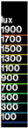 |  | 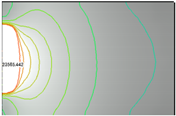 |  |  |
| 921 lx–29,420 lx | 412 lx–23,565 lx | sDA500lx 50% = 80.92% | |||
 V.1.90 |  | 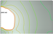 | 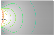 |  |  |
| 572 lx–28,667 lx | 366 lx–2140 lx | sDA500lx 50% = 57.62% | |||
 V.2.90 |  |  |  |  |  |
| 663 lx–29,497 lx | 373 lx–2331 lx | sDA500lx 50% = 63.12% | |||
 V.4.90 |  |  | 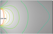 | 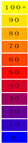 |  |
| 663 lx–28,644 lx | 370 lx–2597 lx | sDA500lx 50% = 65.17% | |||
 V.8.90 |  | 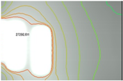 |  |  |  |
| 637 lx–27,292 lx | 357 lx–2283 lx | sDA500lx 50% = 66.62% | |||
 V.16.90 |  |  |  |  | 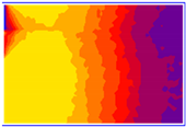 |
| 615 lx–28,465 lx | 356 lx–2191 lx | sDA500lx 50% = 67.21% | |||
| Case | Minimum DF | Maximum DF | Average DF | DF > 2 % | Uniformity Daylight Factor DF min/DF Average |
|---|---|---|---|---|---|
| Reference case | 1.43 | 25.13 | 4.44 | 79 | 0.32 |
| V.1.90 | 1.33 | 15.2 | 3 | 59.17 | 0.44 |
| V.2.90 | 1.29 | 20.76 | 3.51 | 65.42 | 0.37 |
| V.4.90 | 1.29 | 11.8 | 3.26 | 70.21 | 0.40 |
| V.8.90 | 1.35 | 9.19 | 2.98 | 67.25 | 0.45 |
| V.16.90 | 1.42 | 9.84 | 3.01 | 68.88 | 0.47 |
| Case | Illuminance | Daylight Autonomy DA500 | |||
|---|---|---|---|---|---|
| 21 December—12h00 | 21 June—12h00 | ||||
 Reference case |  | 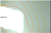 | 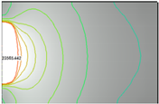 |  |  |
| 921 lx–29,420 lx | 412 lx–23,565 lx | sDA500lx 50% = 80.92% | |||
 V.8.90 |  |  | 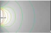 |  | 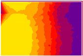 |
| 637 lx–27,292 lx | 357 lx–2283 lx | sDA500lx 50% = 66.62% | |||
 V.8.60 |  |  | 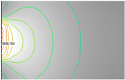 |  |  |
| 534 lx–27,084 lx | 350 lx–1938 lx | sDA500lx 50% = 58.46% | |||
 V.8.120 |  |  | 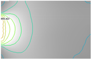 |  | 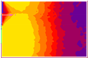 |
| 668 lx–28,578 lx | 256 lx–1665 lx | sDA500lx 50% = 62.33% | |||
| Case | Minimum DF | Maximum DF | Average DF | DF > 2 % | Uniformity Daylight Factor DF min/DF Average |
|---|---|---|---|---|---|
| Reference case | 1.43 | 25.13 | 4.44 | 79 | 0.32 |
| V.8.90 | 1.35 | 9.19 | 2.98 | 67.25 | 0.45 |
| V.8.60 | 1.35 | 7.31 | 2.59 | 57.00 | 0.52 |
| V.8.120 | 1.32 | 11.4 | 3.3 | 67.12 | 0.40 |
| Case | Illuminance | Daylight Autonomy DA500 | |||
|---|---|---|---|---|---|
| 21 December—12h00 | 21 June 21st—12h00 | ||||
 V.8.90 |  | 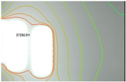 | 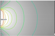 |  |  |
| 637 lx–27,292 lx | 357 lx–2283 lx | sDA500lx 50% = 66.62% | |||
 H.8.45 |  |  |  |  |  |
| 587 lx–28,950 lx | 373 lx–2649 lx | sDA500lx 50% = 58.50% | |||
 H.8.135 |  |  |  |  |  |
| 706 lx–28,930 lx | 358 Lx–2239 lx | sDA500lx 50% = 62.33% | |||
| Case | Minimum DF | Maximum DF | Average DF | DF > 2 % | Uniformity Daylight Factor DF min/DF Average |
|---|---|---|---|---|---|
| V.8.90 | 1.35 | 9.19 | 2.98 | 67.25 | 0.45 |
| H.8.45 | 1.22 | 20.47 | 3.44 | 56.38 | 0.35 |
| H.8.135 | 1.21 | 16.02 | 3.12 | 57.00 | 0.39 |
Publisher’s Note: MDPI stays neutral with regard to jurisdictional claims in published maps and institutional affiliations. |
© 2021 by the authors. Licensee MDPI, Basel, Switzerland. This article is an open access article distributed under the terms and conditions of the Creative Commons Attribution (CC BY) license (https://creativecommons.org/licenses/by/4.0/).
Share and Cite
Magri Elouadjeri, S.; Boussoualim, A.; Ait Haddou, H. Evaluating the Effect of External Horizontal Fixed Shading Devices’ Geometry on Internal Air Temperature, Daylighting and Energy Demand in Hot Dry Climate. Case Study of Ghardaïa, Algeria. Buildings 2021, 11, 348. https://doi.org/10.3390/buildings11080348
Magri Elouadjeri S, Boussoualim A, Ait Haddou H. Evaluating the Effect of External Horizontal Fixed Shading Devices’ Geometry on Internal Air Temperature, Daylighting and Energy Demand in Hot Dry Climate. Case Study of Ghardaïa, Algeria. Buildings. 2021; 11(8):348. https://doi.org/10.3390/buildings11080348
Chicago/Turabian StyleMagri Elouadjeri, Sahar, Aicha Boussoualim, and Hassan Ait Haddou. 2021. "Evaluating the Effect of External Horizontal Fixed Shading Devices’ Geometry on Internal Air Temperature, Daylighting and Energy Demand in Hot Dry Climate. Case Study of Ghardaïa, Algeria" Buildings 11, no. 8: 348. https://doi.org/10.3390/buildings11080348
APA StyleMagri Elouadjeri, S., Boussoualim, A., & Ait Haddou, H. (2021). Evaluating the Effect of External Horizontal Fixed Shading Devices’ Geometry on Internal Air Temperature, Daylighting and Energy Demand in Hot Dry Climate. Case Study of Ghardaïa, Algeria. Buildings, 11(8), 348. https://doi.org/10.3390/buildings11080348