Identification of Environmental and Contextual Driving Factors of Air Conditioning Usage Behaviour in the Sydney Residential Buildings

Abstract

Air conditioning (A/C) is generally responsible for a significant proportion of total building energy consumption. However, occupants’ air conditioning usage patterns are often unrealistically characterised in building energy performance simulation tools, which leads to a gap between simulated and actual energy use. The objective of this study was to develop a stochastic model for predicting occupant behaviour relating to A/C cooling and heating in residential buildings located in the Subtropical Sydney region of Australia. Multivariate logistic regression was used to estimate the probability of using A/C in living rooms and bedrooms, based on a range of physical environmental (outdoor and indoor) and contextual (season, day of week, and time of day) factors observed in 42 Sydney region houses across a two-year monitoring period. The resulting models can be implemented in building energy performance simulation (BEPS) tools to more accurately predict indoor environmental conditions and energy consumption attributable to A/C operation.

1. Introduction

Energy consumption of the residential building sector accounts for approximately 30% of that consumed across all sectors [1]. According to the Department of the Environment and Energy’s latest estimates of Australian energy end-use, space conditioning represents a major component of residential energy consumption nationally. In effect, space heating and water heating constitute the greatest part of the end use in terms of residential total energy consumption in Australia [2]. With the aim of reducing energy consumed for space conditioning, residential buildings are subject to relevant energy efficiency performance requirements, in the form of a star rating system [3]. As in other jurisdictions, building energy performance simulation (BEPS) tools have become the default method for predicting the performance of residential designs, along with energy efficiency compliance assessment in Australia.

BEPS tools predict the energy use of a building based on a series of assumptions regarding building occupant behaviour profiles (e.g., window and shading adjustments, HVAC system operation, etc.). However, such behaviour profiles often inadequately represent actual occupants’ behaviours [4], leading to a gap between the simulated and actual energy use (e.g., [5,6,7,8,9]). For example, the Australian study by CSIRO researchers [10] investigated the thermal performance and cooling/heating energy use in a sample of 414 houses located in three capital cities and climate zones of Australia. While the result confirmed that there was a 19% to 50% reduction in the actual heating energy use in homes with higher thermal performance star-ratings compared to those with lower ratings, there was an inverse correlation between cooling energy use and thermal performance rating. The average cooling energy use in summer was paradoxically greater in homes with higher thermal performance for two of the three cities studied, notwithstanding the similarity in the indoor temperatures observed in both lower- and higher-rated homes. The results underscore a need to narrow the gap between simulated and actual energy use in residential applications.

Implementing more realistic occupant behaviour profiles in BEPS tools would certainly improve the validity of the simulation outcomes, and, in response, research activities aiming at modelling real patterns of occupant behaviour have become more common in the last decade or so (e.g., [11,12,13,14,15,16,17]). Tanimoto and Hagishima [11] used a Markov chain to build a probability model for determining A/C state transition (shifting from off-to-on state and vice versa). The model only used indoor globe temperature (a proxy for operative temperature), ignoring other factors such as the time of day and events. As a result, the Markov chain model could not be applied to actual simulation practice. Another observational study [12] collected behavioural data from over thirty apartments located in different climate zones within China. They developed a probability model using discrete three-parameter Weibull distribution. Yao [13] developed behaviour models for predicting A/C cooling state based on observations from a single, typical apartment located in China using logistic regression as a function of outdoor and indoor temperatures. Bruce-Konuah et al. [14] developed stochastic models of heating override behaviour using logistic regression based on indoor and outdoor physical environment and time of the day factor. The results reported factors other than indoor and outdoor temperatures could act as drivers of A/C usage patterns. Andersen et al. [15] implemented window opening [16] and heating set-point adjustments’ [17] behaviour models developed from the previous study in a BEPS tool enabling stochastic predictions. However, the result showed that the models did not predict the actual indoor environmental conditions well.

Generally, most of the previously published studies relied exclusively upon indoor and outdoor temperatures as predictor variables to infer A/C state, but some have investigated the impact of non-thermal, contextual factors such as outdoor environmental conditions and time of day to enhance model validity. The study by Bruce-Konuah [14] reported that factors other than indoor and outdoor temperatures can also be a key driver for occupants to operate A/C. Thus, a general consensus seems to be emerging in the literature regarding the complexity of influences on residential occupants’ A/C use behaviour.

Furthermore, the majority of previous studies developed models that predict the A/C state itself, i.e., either turned on or off, rather than the change-of-state (i.e., turning off-to-on or vice versa). This becomes problematic if the predictor variables used in the model are influenced by the state of the A/C. In winter, for example, high indoor temperatures would be monitored when A/C heating is turned on and not when A/C is turned off. The analysis in such a case would lead to the counterintuitive observations of A/C heating being turned off with decreasing indoor temperatures, and to be turned on with increasing indoor temperatures. This problem can be overcome by modelling the change of A/C state (turned off-to-on or vice versa) rather than the state per se. This approach should reveal the variables most relevant to A/C turning on behaviour and turning off behaviour, separately.

The research literature also indicates that occupant behaviour can vary widely depending on context [18,19,20]. This is presumably because occupant behaviour is not simply deterministic, but rather the result of myriad, interacting factors including cultural norms, climatic setting, building design, and adaptive comfort opportunities available within the building. The main objective of the current study is to develop stochastic models for predicting A/C cooling and heating use behaviours in Australian residential buildings based on longitudinal field observations of physical environmental (outdoor and indoor) and contextual (season, day of week and time of day) factors as well as A/C use behaviour in living rooms and bedrooms.

2. Materials and Methods

2.1. Samples

A total of 42 households in two adjacent cities on Australia’s eastern seaboard, Sydney and Wollongong, participated in the study. Both cities fall within the humid sub-tropical climate zone of eastern Australia and so, for the purposes of this study, can be regarded as a single sample. Field measurements were conducted across two years, from March 2012 through March 2014. Indoor air temperature and humidity were recorded every 15 min for the duration of the study at various locations within the occupied zones of each participating house (including living room, bedroom, dining room, kitchen, and study) using iButtons (accuracy ±0.5 °C, ±5% RH) [21]. The iButtons were installed at about 0.6–0.8 m above the floor level, e.g., underneath the tables, desk or cabinets, to avoid exposure to direct sunlight. iButtons were also placed on the air outlet of the air conditioning system or fan-coil unit.

The delta-temperature between the A/C supply outlet and the occupied zone has been previously used to determine when A/C was operational using the iButton’s 15-min logging interval [22]. First, if the difference between two sequential supply air temperature measurements was greater than 3.5 K, then the A/C was considered to be switched on within that 15-min period. The temperature in the occupied zone when the A/C was operational and two subsequent measurements were analysed in consideration of thermal capacity of the sensor. If the difference between the maximum of the three temperatures in the occupied zone and the supply air temperature was greater than the threshold specified for that house (nominally 3 K but adjusted to individual cases), then heating was deemed to be in use. If not, the same logic was applied to the minimum of the three measurements to test if cooling was being used. This logic was continued until neither case was true and then the A/C was flagged as not in use. This method was applied to the observations made in the current study; 30 living rooms, 15 bedrooms, 6 dining rooms, 6 study rooms, 3 kitchens, and 2 lounges across the participating households. We believed the sample sizes of the occupied zones other than the living room and bedroom were too small to be representative of typical Australian households. For this reason, this study excluded data from households who installed iButtons in the occupied zones other than the living room and bedroom. As a result, the data set used in this study consists of the measurements in the 30 living rooms and 15 bedrooms from the 36 participants’ homes.

The main features of the houses and their occupants are summarised in

Table 1. Description of the sample of Sydney region residents and characteristics of their houses.

House Index	Number of Residents	Average Age of the Residents	Number of Storeys	House Construction	Participation Duration (Years)	IEQ Sensor Location	Participating Season a
1	4	19	Two Storey	Double brick	0.8	Living	SMR/AUT/ WIN
2	2	35	Other	Other	0.7	Living/Bed	SMR/AUT/ WIN
3	4	19	One storey	Brick veneer	1.5	Living	SPG/SMR/ AUT/WIN
4	2	35	One storey	Double brick	0.3	Living	SPG/WIN
5	2	35	One storey	Lightweight cladding	0.3	Living/Bed	SPG/SMR
6	2	35	Other	Double brick	0.6	Living	SPG/SMR/ AUT
7	3	40	One storey	Brick veneer	2.1	Living/Bed	SPG/SMR/ AUT/WIN
8	3	40	Split level	Timber	2.1	Bed	SPG/SMR/ AUT/WIN
9	2	35	Other	Double brick	1.1	Living/Bed	SPG/SMR/ AUT/WIN
10	3	45	One storey	Double brick	2.1	Living	SPG/SMR/ AUT/WIN
11	5	25	Two Storey	Composite	1.6	Living	SPG/SMR/ AUT/WIN
12	4	33	Two Storey	Brick veneer	1.6	Bed	SPG/SMR/ AUT/WIN
13	2	30	Other	Other	0.3	Living	SPG/WIN
14	2	65	Other	Other	0.6	Living/Bed	SPG/SMR/ AUT
15	6	38	Split level	Composite	0.3	Bed	SPG/SMR
16	4	41	Two Storey	Double brick	2.1	Living/Bed	SPG/SMR/ AUT/WIN
17	2	30	One storey	Brick veneer	2.1	Living/Bed	SPG/SMR/ AUT/WIN
18	4	32	One storey	Other	1.8	Living	SPG/SMR/ AUT/WIN
19	2	35	One storey	Double brick	1.5	Living	SPG/SMR/ AUT
20	3	24	Other	Lightweight cladding	1.7	Living	SPG/SMR/ AUT/WIN
21	2	35	One storey	Other	1.8	Living/Bed	SPR/WIN
22	-	-	Other	Other	1.3	Bed	SMR/AUT
23	4	24	One storey	Brick veneer	2.1	Living	SPG/SMR/ AUT/WIN
24	6	33	Two Storey	Brick veneer	2.1	Living	SPG/SMR/ AUT/WIN
25	5	30	Other	Double brick	0.8	Living	SPR/SMR/ AUT
26	2	35	Other	Double brick	1.4	Living	SPG/SMR/ AUT/WIN
27	2	60	Two Storey	Double brick	1.3	Bed	SMR/AUT
28	3	34	Two Storey	Composite	1.2	Living	SPG/SMR/ AUT/WIN
29	2	55	Split level	Brick veneer	1.2	Bed	SPG/SMR/ AUT/WIN
30	2	45	One storey	Brick veneer	1.2	Living	SPG/SMR/ AUT/WIN
31	4	28	One storey	Brick veneer	0.8	Living	SPG/SMR/ AUT/WIN
32	2	65	Two Storey	Brick veneer	1.1	Living/Bed	SPG/SMR/ AUT/WIN
33	4	19	One storey	Timber	1.1	Living	SPG/SMR/ AUT/WIN
34	4	21	One storey	Brick veneer	1.1	Living	SPG/SMR/ AUT/WIN
35	2	60	Split level	Other	0.8	Living	SPG/SMR/ AUT/WIN
36	4	21	Two Storey	Composite	0.9	Living	SPG/SMR/ AUT/WIN

^a SPG, spring; SMR, summer; AUT, autumn; WIN, winter.

. Most of our house samples comprised masonry construction (double brick 27.8% or brick veneer 30.6%), and 25 houses (69.4%) had ceiling insulation. The most common house type was single storey (38.9%), followed by double storey (25%), and then split-level (11.1%). The most common number of occupants in the houses were 2 persons (45.7%), 4 persons (28.6), 3 persons (14.3%) and more than 4 persons (11.4%).

A/C usage behaviour is known to be weather sensitive [14,22,23]. Concurrent meteorological observations (excluding solar radiation) were obtained from the nearest official Australian Bureau of Meteorology (BOM) stations. Generally, all houses in the sample fell within a 7 km radius of the closest BOM stations. Concurrent solar radiation observations were obtained from the Department of Environmental Sciences Automatic Weather Station at Macquarie University [24].

2.2. Preparation and Processing of Data

Simultaneous outdoor and indoor environmental data were merged to build a 15-min resolution dataset. Regarding the dependent variables for modelling, A/C cooling and heating states were coded as binary variables for each 15-min time step. When A/C state change occurred (off to on/on to off), the immediately preceding time step was flagged as a state-change event. For example, if A/C was turned on at 10:00 a.m., 9:45 a.m. was coded as a ‘turning on’ event. Four possible state codes comprised ‘turned off’, ‘turning on’, ‘turned on’ and ‘turning off’ for both cooling and heating modes of operation (referred to as ‘cooling action’ and ‘heating action’). Therefore, the data set was filtered depending on the purpose of the four A/C usage models (i.e., cooling on, cooling off, heating on, and heating off). For example, data with ‘turned off’ and ‘turning on’ for cooling action were used for developing a cooling on model that represents the probability of A/C being turned from off to on at the next time step.

Table 2. List of explanatory variables.

Variable	Unit
Categorical
Season	Summer/Winter/Intermediate
Day of week	Weekday/Weekend
Time of day	Night/Morning/Afternoon/Evening
Continuous
Outdoor air temperature (To)	°C
Outdoor relative humidity (RHo)	%
Solar radiation (Rad)	W/m2
Wind speed (WS)	m/s
Rainfall (RF)	mm
Prevailing mean outdoor temperature (PMA)	°C
Indoor air temperature (Ti)	°C
Indoor relative humidity (RHi)	%

lists all the variables used to derive A/C usage models. Thus, three categorical variables were computed to capture different behavioural patterns, depending on season (summer/winter/intermediate), day-of-week (weekday/weekend) and time-of-day (night/morning/afternoon/evening). Outdoor and indoor environmental parameters were represented as continuous variables. The prevailing mean outdoor air temperature (PMA) was also calculated based on the weighted 7-day running mean method defined in ASHRAE Standard 55 [25]. Logarithmic transformation was applied to solar radiation, wind speed, and rainfall observations to obtain a more normalised distribution, as shown in

Table 3. Variable transformation. Log indicates the natural logarithm.

Variable	Unit
Solar radiation (W/m2)	Log(Solar radiation + 1) (Log(W/m2))
Wind speed (m/s)	Log(Wind speed + 1) (Log(m/s))
Rainfall (mm)	Log(Rainfall + 1) (Log(mm))

.

2.3. Statistical Analysis

Multivariate logistic regression was used to develop the A/C usage models as it has been widely adopted in modelling occupant behaviour [13,14,16]. The probability function can be expressed as follows:

$$\log \left(\frac{p}{1-p}\right)=a+b_1{x}_1+b_2{x}_2+\cdots +b_n{x}_n$$

(1)

where p is the probability of turning on/off A/C; a is the intercept; b is the coefficient; and x is the explanatory variables.

The monitored A/C usage behaviours in the living room and bedroom were different, as shown in Figure 1. Thus, the fitted regression coefficients differed. For example, an increase in solar radiation might increase the probability of an A/C turning on in the living room, but the same increase might result in a smaller increment in bedroom A/C probability. This is because the A/C in the living room was usually turned on during the daytime, whereas an A/C in the bedroom was turned on more frequently in the night-time. Consequently, A/C usage behaviours in the living room and bedroom were modelled separately, suggesting 8 (2 × 2 × 2) different models, i.e., cooling/heating, turning on/off, in the living room/bedroom.

The explanatory variables selected in each model were determined based on a forward and backward selection using the Akaike Information Criterion (AIC). The procedure begins from the null model and adds in variables one by one (forward selection). The AIC is calculated for each case, and the variable with the lowest AIC is selected. The remaining variables are then tested one by one again with the selected variable. If the bivariate model has a higher AIC than the univariate model, the univariate model is chosen. However, if the bivariate model has a lower AIC, the procedure progresses to a three variable model, and so on. At each step, the AIC for models obtained by removing each of the selected variables are also calculated for comparison (backward selection). For example, additional three bivariate models can be obtained from a three variables model. This process continued with the same criteria, up to n variables models.

To evaluate the influence of explanatory variables within each model, the coefficient should be taken into account with the scale. Schweiker and Shukuya [26] suggested the absolute value of the coefficient multiplied by the scale of the explanatory variable (max-min value), to get an indication of the magnitude of the impact of each variable on the overall model. For example, the magnitude of the impact of solar radiation on A/C cooling turning on and turning off behaviours in living rooms were 0.4 ($\left|0.051\times 7.1\right|$) and 0.9 ($\left|-0.124\times 7.1\right|$), respectively.

Logistic regression assumes negligible collinearity amongst the explanatory variables because it inflates the estimated variance accounted by the inferred coefficients of the variables contained in the model. Accordingly, possible inflation of the estimated variance due to multicollinearity was assessed for all variables in each model using a generalised variance inflation factor (GVIF). A GVIF of 1 indicates that there is no correlation between the explanatory variables. A GVIF between 1 and 5 indicates a moderate correlation, and over 5 denotes a high correlation. Generally, a GVIF of 10 was recognised as the maximum acceptable level, but the value of 4 has been recommended [27]. The GVIF^1/(2×Df) was calculated to estimate the inflation of the variance due to multicollinearity. The GVIF values for all the explanatory variables contained in cooling and heating usage models are presented respectively in

Table 4. GVIF analysis results from A/C Cooling on and off models.

Variable	Cooling On			Cooling Off
	GVIF	Df	GVIF1/(2×Df)	GVIF	Df	GVIF1/(2×Df)
Living
Season	1.8	2	1.2
Day of week	1	1	1
Time of day	7	3	1.4	6.9	3	1.4
Rad	6.5	1	2.6	6.3	1	2.5
RF	1	1	1
WS	1.3	1	1.1	1.3	1	1.1
PMA	1.9	1	1.4	1.3	1	1.1
To	4.9	1	2.2	3.6	1	1.9
RHo	3.8	1	2	4.8	1	2.2
Ti	2	1	1.4	1.2	1	1.1
RHi				2	1	1.4
Bed
Season	2.8	2	1.3	2.3	2	1.2
Day of week	1	1	1
Time of day	1.6	3	1.1	10.1	3	1.5
Rad				6.4	1	2.5
RF				1.1	1	1
WS	1.3	1	1.2	1.6	1	1.3
PMA	3.1	1	1.7
To	1.8	1	1.3	5.3	1	2.3
RHo				7.1	1	2.7
Ti				3.5	1	1.9
RHi	1.3	1	1.1	4.9	1	2.2

and

Table 5. GVIF analysis result from A/C Heating on and off models.

Variable	Heating On			Heating Off
	GVIF	Df	GVIF1/(2×Df)	GVIF	Df	GVIF1/(2×Df)
Living
Season	3	2	1.3	2.9	2	1.3
Day of week	1	1	1
Time of day	3	3	1.2	5.4	3	1.3
Rad	2.4	1	1.6	4.3	1	2.1
RF	1.1	1	1.1
WS	1.5	1	1.2	1.1	1	1.1
PMA	3.3	1	1.8	3	1	1.7
To	4.4	1	2.1	1.8	1	1.3
RHo	3.1	1	1.8
Ti	2.3	1	1.5	1.3	1	1.1
RHi	1.9	1	1.4
Bed
Season	7	2	1.6
Time of day	3.2	3	1.2	8.5	3	1.4
Rad	2.6	1	1.6	5.8	1	2.4
WS	1.2	1	1.1	1.2	1	1.1
PMA	7.4	1	2.7	2.7	1	1.6
To	3.5	1	1.9	3.7	1	1.9
Ti	1.7	1	1.3	2.1	1	1.5
RHi	1.2	1	1.1

. The values were all less than 4, indicating the level of the inflation of the estimated variance of the coefficients was acceptable.

All statistical analysis described in this paper was conducted in R version 3.6.3 [28].

3. Results

Following the procedure described above, a total of eight A/C usage behaviour models, i.e., cooling/heating turning on and off in a living room and bedroom, were developed.

Table 6. Descriptive statistics of monitored data.

	To	RHo	Rad	WS	RF	PMA	Ti		RHi
							Living Room	Bed-Room	Living Room	Bed-Room
A/C Off
Max	45.9	100	1218.9	74	25.8	25.3	43.1	47.1	91.7	91.5
3rd quarter	22	84	319.2	17	0	21.7	24.6	24.7	66.8	66.4
Mean	18.4	68.8	183.5	11.4	0	18.4	21.6	21.7	57.6	55.1
Median	18.8	70	5.5	10	0	19	21.7	22.1	58.9	56.4
1st quarter	14.9	56	0	5	0	15.3	19.1	18.7	50.1	44.9
Min	−2.2	4	0	0	0	8.5	9.1	5.6	12.4	12.5
A/C Cooling on
Max	45.9	100	1154	63	18	25.3	36.2	36.6	91.5	91.5
3rd quarter	27.4	76	350.3	22	0	23.2	26.2	25.2	61.1	85.1
Mean	25.6	61.5	206.2	15.4	0	22.1	24.7	23.2	54.8	69.7
Median	24.6	65	14	15	0	22.5	24.6	23.1	54.1	70.9
1st quarter	22.5	51	0	9	0	21.6	23.2	21.2	47.6	59
Min	5.8	7	0	0	0	11.3	14.1	11.6	14.9	12.5
A/C Heating on
Max	36.3	100	1013.8	59	6.4	25.3	35.7	37.7	91.5	91.5
3rd quarter	14.5	89	43.9	15	0	13.9	21.6	19.7	60.9	65.7
Mean	12.6	70.8	73.8	11	0.1	13.3	19.7	16.7	50.4	51.8
Median	12.5	71	0	9	0	12.8	19.6	15.6	52	51.2
1st quarter	10.7	55	0	5	0	12	17.2	13.1	41	37.5
Min	−0.2	10	0	0	0	8.5	10.1	9.1	12.5	12.5

presents descriptive statistics of all the variables used in each of the A/C usage behaviour models.

Table 7. Coefficients and magnitudes of variables inferred from cooling on and off models.

Variables	Cooling On				Cooling Off
	Coefficient	Confidence Interval		Magnitude	Coefficient	Confidence Interval		Magnitude
		2.50%	97.50%			2.50%	97.50%
Living room
Intercept	−17.881	−18.956	−16.822		1.481	0.349	2.603
Summer	0.224	0.044	0.408
Winter	−0.976	−2.178	−0.072
Weekend	0.326	0.199	0.451
Evening	0.637	0.34	0.931		−0.123	−0.439	0.189
Morning	−0.563	−0.775	−0.358		0.233	−0.049	0.505
Night	−1.398	−1.928	−0.905		−0.44	−0.844	−0.042
Rad	0.051	−0.004	0.107	0.4	−0.124	−0.183	−0.066	0.9
RF	−1.071	−2.179	−0.213	3.5
WS	0.135	0.041	0.231	0.6	−0.082	−0.171	0.009	0.3
PMA	0.134	0.092	0.177	2.3	−0.079	−0.118	−0.039	1
To	0.173	0.15	0.195	8.3	−0.103	−0.13	−0.075	3.6
RHo	0.009	0.004	0.015	0.9	−0.022	−0.029	−0.014	2
Ti	0.139	0.114	0.164	4.7	0.04	0.01	0.07	0.9
RHi					0.029	0.022	0.036	2.2
Bedroom
Intercept	−14.813	−16.081	−13.58		0.309	−1.158	1.764
Summer	0.417	0.178	0.664		0.115	−0.145	0.382
Winter	0.931	0.316	1.523		0.832	0.073	1.595
Weekend	0.38	0.215	0.543
Evening	0.786	0.577	0.997		0.152	−0.305	0.603
Morning	−0.423	−0.698	−0.155		0.551	0.206	0.894
Night	0.038	−0.288	0.357		−0.037	−0.542	0.463
Rad					0.074	−0.009	0.157	0.5
RF					0.906	0.15	1.577	2.2
WS	−0.098	−0.194	0.001	0.4	−0.156	−0.256	−0.055	0.6
PMA	0.162	0.1	0.225	2.6
To	0.181	0.162	0.201	8.4	−0.195	−0.247	−0.145	7.8
RHo					−0.012	−0.025	0.001	1.1
Ti					0.153	0.103	0.204	3.8
RHi	0.01	0.004	0.016	0.8	−0.009	−0.02	0.002	0.7

and

Table 8. Coefficients and magnitudes of variables inferred from heating on and off models.

Variables	Heating On				Heating Off
	Coefficient	Confidence Interval		Magnitude	Coefficient	Confidence Interval		Magnitude
		2.50%	97.50%			2.50%	97.50%
Living room
Intercept	−0.639	−1.465	0.183		−4.854	−5.771	−3.939
Summer	−0.138	−0.565	0.264		0.777	0.226	1.321
Winter	0.819	0.611	1.032		0.17	−0.041	0.385
Weekend	−0.12	−0.248	0.006
Evening	−0.795	−0.983	−0.604		0.516	0.257	0.784
Morning	−0.627	−0.813	−0.441		0.728	0.498	0.961
Night	−2.169	−2.431	−1.911		1.142	0.821	1.466
Rad	−0.237	−0.273	−0.201	1.7	0.097	0.047	0.148	0.7
RF	0.473	0.026	0.864	1.6
WS	0.141	0.076	0.206	0.6	−0.165	−0.223	−0.106	0.7
PMA	−0.103	−0.14	−0.066	1.7	0.081	0.032	0.129	1.3
To	−0.075	−0.1	−0.05	3.6	0.039	0.016	0.063	1.4
RHo	−0.018	−0.023	−0.013	1.7
Ti	−0.132	−0.16	−0.104	4.5	0.027	0.008	0.046	0.6
RHi	0.022	0.016	0.028	1.7
Bedroom
Intercept	−0.548	−1.781	0.677		−4.298	−4.964	−3.646
Summer	1.147	0.696	1.605
Winter	0.58	0.235	0.937
Evening	−0.692	−0.991	−0.387		0.618	0.195	1.066
Morning	−0.118	−0.375	0.138		0.024	−0.301	0.352
Night	−2.332	−2.817	−1.875		1.138	0.543	1.738
Rad	−0.187	−0.239	−0.135	1.3	0.095	0.012	0.181	0.7
WS	0.125	0.028	0.223	0.5	−0.128	−0.234	−0.021	0.5
PMA	−0.14	−0.207	−0.073	2.3	0.157	0.101	0.214	2.4
To	0.042	0.008	0.075	2	0.084	0.043	0.127	2.9
Ti	−0.254	−0.281	−0.227	10.5	−0.06	−0.093	−0.029	1.5
RHi	0.01	0.005	0.015	0.8

present the coefficients, their confidence interval estimates, and magnitudes of the impact of each variable on the overall model included in the cooling and heating models respectively. The coefficients, ‘season-intermediate’, ‘day of week-weekday’ and ‘time of day-afternoon’ are missing because they are used as references for the corresponding categorical variables.

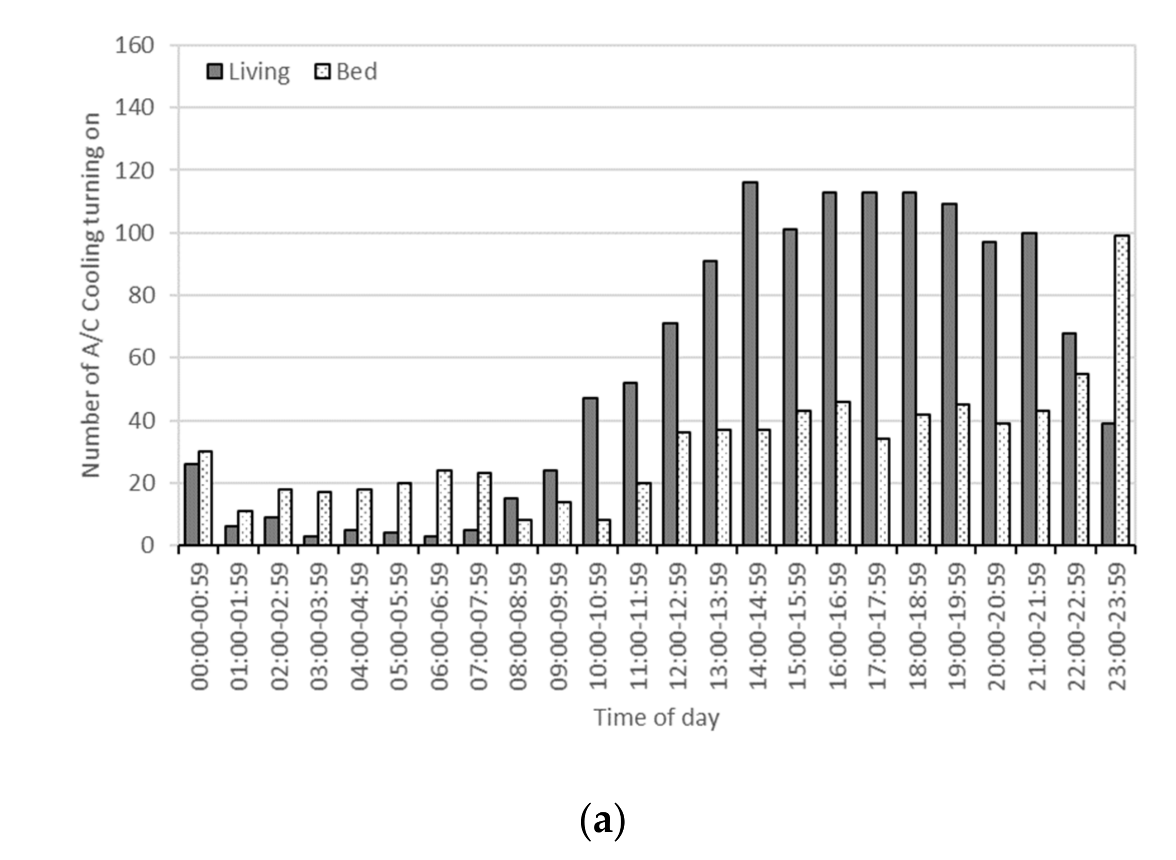
3.1. A/C Cooling Behaviour—‘Cooling On’

On the basis of the magnitudes of the impact of explanatory variables on the overall model, the most influential variable on A/C cooling turning on behaviour was the outdoor air temperature in both spaces, i.e., living rooms and bedrooms. Outdoor temperature and PMA (prevailing mean outdoor air temperature) were positively correlated with the probability of ‘cooling on’. Indoor air temperature and rainfall had positive and negative effects respectively on the probability of ‘cooling on’, while they did not have a significant influence in the bedroom. Indoor relative humidity was the only variable removed among the explanatory variables in the living room, whereas four continuous variables, i.e., RH_o, Rad, RF and T_i, were removed in the bedroom. All the categorical variables were all significant in both areas.

Equations can be generated using the coefficients and intercepts listed in Table 7 and Table 8. The two equations below describe the probability of ‘A/C cooling on’ occurring during summer mornings on weekdays in the living room (2) and bedroom (3):

$$\log \left(\frac{\mathrm{p}}{1-\mathrm{p}}\right)=-18.22+0.051 \log \left(\mathrm{Rad}+1\right)-1.071 \log \left(\mathrm{RF}+1\right)+0.135 \log \left(\mathrm{WS}+1\right)+0.134 \mathrm{PMA}+0.173{ \mathrm{T}}_{\mathrm{o}}+0.009{ \mathrm{RH}}_{\mathrm{o}}+0.139{ \mathrm{T}}_{\mathrm{i}}$$

(2)

$$\log \left(\frac{\mathrm{p}}{1-\mathrm{p}}\right)=-14.82-0.098 \log \left(\mathrm{WS}+1\right)+0.162 \mathrm{PMA}+0.181{ \mathrm{T}}_{\mathrm{o}}+0.01{ \mathrm{RH}}_{\mathrm{i}}$$

(3)

where

p is the probability of turning on A/C (cooling mode) in the next 15 min,

Rad is the solar radiation in W/m²,

RF is the total amount of rainfall in last 15 min in mm,

WS is the wind speed in m/s,

PMA is the prevailing mean outdoor air temperature in °C,

T_o and T_i are the outdoor and indoor air temperature in °C,

RH_o and RH_i are the outdoor and indoor relative humidity in %.

3.2. A/C Cooling Behaviour—‘Cooling Off’

Outdoor air temperature was again found to be the most important variable associated with ‘cooling off’ behaviour in both living rooms and bedrooms. While outdoor air temperature had a negative correlation in both spaces, indoor air temperature had a positive correlation. All of the continuous variables had a significant effect on the probability of ‘cooling off’ behaviour, except rainfall for the living room and PMA for the bedroom. Solar radiation and indoor relative humidity had negative and positive impacts, respectively, in the living room, and opposite effects in bedrooms. Regarding the impact of the contextual categorical variables on ‘cooling off’ behaviour, season was removed from the living room, and day of week was removed from both the living rooms and bedrooms.

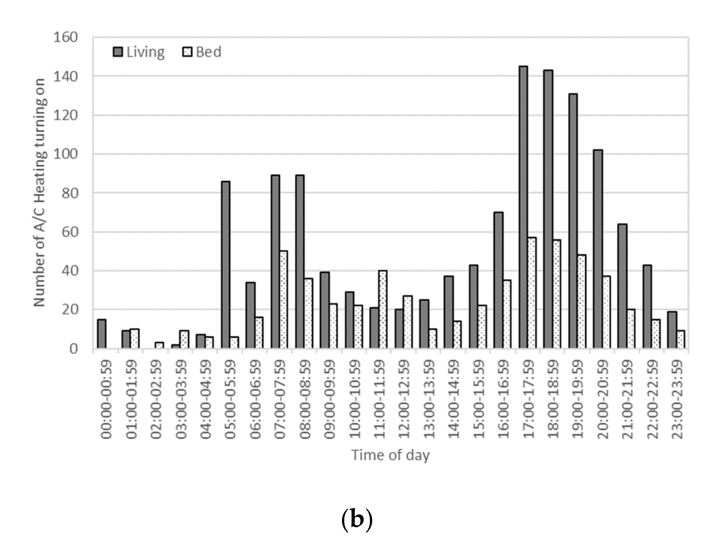
3.3. A/C Heating Behaviour—‘Heating On’

All of the variables were statistically significant for determining ‘heating on’ behaviour in the living room, whereas rainfall, outdoor relative humidity, and day of week effects were removed from the bedroom model. Unlike ‘cooling’ behaviour models where outdoor air temperature was most influential, it was indoor air temperature that was most important for the ‘heating’ behaviour models. Indoor and outdoor air temperature and PMA were all negatively correlated with the probability of turning heating on in the living room, but the sign of the outdoor air temperature coefficient turned out to be positive in the bedroom.

3.4. A/C Heating Behaviour—‘Heating Off’

Rainfall, outdoor relative humidity, indoor relative humidity, and day of week all dropped out of the ‘heating off’ models in both bedrooms and living rooms, as did the seasonal effect for the bedroom model. The most important drivers for ‘heating off’ behaviour were outdoor and indoor air temperatures as well as PMA. Counterintuitively, indoor air temperature turned out to have a smaller influence than outdoor air temperature on ‘heating off’ behaviour. Other continuous variables had a relatively smaller impact on heating off behaviour.

3.5. Generalisations across All of the Heating and Cooling Behaviour Models

Different explanatory variables exerted different effects on the various A/C behaviour models. Generally, outdoor air temperature was identified as the most significant driver for all A/C behaviour models, with the exception being the ‘heating turning on’ model where indoor air temperature was the dominant driver. PMA was consistently influential in all models. Solar radiation and wind speed were statistically significant for all models, but the size of their impacts was relatively minor. Rainfall and outdoor and indoor relative humidity were not always related to A/C behaviour, but they had significant impacts on some behaviours. Regarding the effect of categorical variables, ‘season’ and ‘time of day’ had impact in almost all models. ‘Day of week’ did not affect ‘turning off’ behaviour in bedrooms or living rooms.

4. Discussion

The results of our analysis indicate that occupants’ control actions relating to A/C in heating and cooling modes in residential settings were driven by various combinations of environmental and contextual variables. The impact of explanatory variables on the A/C control behaviour varied depending on the A/C modes (cooling/heating), behaviour type (turning on/off) and room type (living room/bedroom). It seems clear that variables other than the conventional choices, outdoor and indoor air temperature, should be taken into consideration when developing more realistic and nuanced occupant behaviour schedules for application in building energy simulation.

Outdoor air temperature emerged from this analysis as the most influential driver for the ‘cooling on/off’ and ‘heating off’ behaviours, except for the ‘heating on’ model, where indoor air temperature was most influential, as listed in Table 7 and Table 8. In conventional behaviour modelling in building energy simulation, the trigger to turn off the A/C is presumed to be indoor environmental variables; once the A/C has been activated, the occupants are expected to rationally turn off the A/C once indoor environmental conditions have met their comfort expectations [26]. However, the results of our analysis indicate that outdoor air temperature was the overriding influence on both A/C cooling and heating ‘turning off’ actions. Furthermore, the sign (positive or negative) of the indoor air temperature coefficients in the models was opposite to those found for outdoor air temperature. For example, the coefficients of indoor air temperature in the turning A/C cooling ‘off’ models for the living room and bedroom had positive signs, indicating that the probability of turning off the A/C cooling increased as indoor air temperature increases. This is probably because A/C heavy users keep their A/C on for longer at a lower temperature, whereas A/C light users operate their A/C for a short time at a higher indoor air temperature. Thus, clustering and modelling diverse behavioural patterns would represent the diversity of occupants expected to be found in the community.

There was a substantial difference found between the A/C operation patterns of the living rooms and bedrooms, as shown in Figure 1. The A/C cooling in the living room was mostly turned on in the afternoon, whereas the A/C in the bedroom was turned on mostly at night, presumably before sleeping. A/C heating was turned on more frequently during the early morning and evening in the living room as compared to the bedroom. The different usage patterns seem to be strongly related to the occupancy pattern of each room. Behavioural models based on the occupancy state might enable more realistic predictions of A/C operation. Nevertheless, the modelling in this study was conducted without definitive information on the state of occupancy in a given room because accurate of occupancy detection is still a challenge [29] and particularly difficult in the residential context.

This paper provides details of behaviour models estimating the probability of an A/C to be turned on and off based on environmental measurement data collected in Australian residential buildings. We used logistic regression and selected the Akaike information criterion (AIC) as a basis of identifying key variables in the model. The proposed models can be implemented into BEPS tools to more accurately predict indoor environment and energy consumption associated with A/C usage. In our analysis, we treated the whole sample as one group, and other potential influencing factors, such as personal characteristics, social parameters, and building design features, were not considered. Thus, predicting the precise A/C usage behaviour of one specific home was outside the scope of this work. Future research should investigate whether there is a common behaviour pattern for sub-groups categorised by the above-mentioned variables. Such an approach would facilitate the development of models for predicting specific group or population behaviours [30,31].

Various other modelling techniques have been attempted in the literature such as data mining [32,33,34] and agent-based modelling [35]. For example, Chen et al. [36] have developed an agent-based occupancy simulator capable of performing a stochastic simulation of occupant presence and movement in buildings. An agent-base is a computational model to simulate the behaviour of each individual occupant independently and produce respective behaviour patterns. As an agent-based model (ABM) facilitates focus at different levels, from the group level down to the individual level, it is useful for the capture of diverse characteristics of occupants such as psychological and social factors [37]. On the other hand, due to occupant diversity, ABM can significantly increase the computational cost of a large-scale simulation. It also requires special expertise and understanding in settings regarding various occupant behaviours to set appropriate sequences of different behaviours. It should also be noted that the real-time communication between the ABM and BEPS tools may lead to an increase in the difficulty of its application [38].

5. Conclusions

This paper proposed the behavioural models of occupant A/C usage based on longitudinal data collected in Australian homes. Multivariate logistic regression was used to develop the stochastic model, predicting ‘turning on’ and ‘turning off’ actions for A/C cooling/heating operation in the next 15 min in the living room and bedroom, based on a range of physical environmental (outdoor and indoor) and contextual (season, day of week and time of day) factors.

The work reported in this study found that occupant control of A/C in residential buildings was driven by numerous environmental and contextual variables, suggesting that variables other than just outdoor and indoor air temperature should be taken into account. Different A/C usage patterns were observed between the living room and bedroom due to the occupancy state. Consequently, this study has resulted in the development of A/C usage models for both living rooms and bedrooms. The proposed models can be implemented in building energy performance simulation (BEPS) tools to more accurately predict indoor environmental conditions and energy consumption associated with A/C usage.

References

1. Swan, L.G.; Ugursal, V.I. Modeling of end-use energy consumption in the residential sector: A review of modeling techniques. Renew. Sustain. Energy Rev. 2009, 13, 1819–1835. [Google Scholar] [CrossRef]
2. Australia Department of the Environment and Energy. Australian Energy Statistics; Australia Department of the Environment and Energy: Canberra, Australia, 2019.
3. NatHERS. Nationwide House Energy Rating Scheme (NatHERS) 2010. Available online: https://www.nathers.gov.au/ (accessed on 25 September 2020).
4. Mahdavi, A. People in building performance simulation. In Building Performance Simulation for Design and Operation; Hensen, J.L.M., Lamberts, R., Eds.; Spon Press: London, UK, 2011; pp. 56–83. [Google Scholar] [CrossRef]
5. Branco, G.; Lachal, B.; Gallinelli, P.; Weber, W. Predicted versus observed heat consumption of a low energy multifamily complex in Switzerland based on long-term experimental data. Energy Build. 2004, 36, 542–555. [Google Scholar] [CrossRef]
6. Calì, D.; Osterhage, T.; Streblow, R.; Müller, D. Energy performance gap in refurbished German dwellings: Lesson learned from a field test. Energy Build. 2016, 127, 1146–1158. [Google Scholar] [CrossRef]
7. De Wilde, P. The gap between predicted and measured energy performance of buildings: A framework for investigation. Autom. Constr. 2014, 41, 40–49. [Google Scholar] [CrossRef]
8. Park, J.S.; Kim, H.J. A field study of occupant behavior and energy consumption in apartments with mechanical ventilation. Energy Build. 2012, 50, 19–25. [Google Scholar] [CrossRef]
9. Parker, D.; Mills, E.; Rainer, L.; Bourassa, N.; Homan, G.; Berkeley, L. Accuracy of the home energy saver energy calculation methodology. In Proceedings of the 2012 ACEEE Summer Study on Energy Efficiency in Buildings, Pacific Grove, CA, USA, 12–17 August 2012. [Google Scholar]
10. Ambrose, M.; James, M.; Law, A.; Osman, P.; White, S. The Evaluation of the 5-Star Energy Efficiency Standard for Residential Buildings; Commonwealth of Australia: Canberra, Australia, 2013. [Google Scholar]
11. Tanimoto, J.; Hagishima, A. State transition stochastic model for predicting off to on cooling schedule in dwellings as implemented using a multilayered artificial neural network. J. Build. Perform. Simul. 2012, 5, 45–53. [Google Scholar] [CrossRef]
12. Ren, X.; Yan, D.; Wang, C. Air-conditioning usage conditional probability model for residential buildings. Build. Environ. 2014, 81, 172–182. [Google Scholar] [CrossRef]
13. Yao, J. Modelling and simulating occupant behaviour on air conditioning in residential buildings. Energy Build. 2018, 175, 1–10. [Google Scholar] [CrossRef]
14. Bruce-Konuah, A.; Jones, R.V.; Fuertes, A. Physical environmental and contextual drivers of occupants’ manual space heating override behaviour in UK residential buildings. Energy Build. 2019, 183, 129–138. [Google Scholar] [CrossRef]
15. Andersen, R.K.; Fabi, V.; Corgnati, S.P. Predicted and actual indoor environmental quality: Verification of occupants’ behaviour models in residential buildings. Energy Build. 2016, 127, 105–115. [Google Scholar] [CrossRef] [Green Version]
16. Andersen, R.; Fabi, V.; Toftum, J.; Corgnati, S.P.; Olesen, B.W. Window opening behaviour modelled from measurements in Danish dwellings. Build. Environ. 2013, 69, 101–113. [Google Scholar] [CrossRef]
17. Fabi, V.; Andersen, R.V.; Corgnati, S.P. Influence of occupant’s heating set-point preferences on indoor environmental quality and heating demand in residential buildings. HVAC R Res. 2013, 19, 635–645. [Google Scholar] [CrossRef]
18. Jeong, B.; Jeong, J.W.; Park, J.S. Occupant behavior regarding the manual control of windows in residential buildings. Energy Build. 2016, 127, 206–216. [Google Scholar] [CrossRef]
19. Rijal, H.B.; Tuohy, P.; Humphreys, M.A.; Nicol, J.F.; Samuel, A.; Clarke, J. Using results from field surveys to predict the effect of open windows on thermal comfort and energy use in buildings. Energy Build. 2007, 39, 823–836. [Google Scholar] [CrossRef] [Green Version]
20. Nicol, J.F. Characterising occupant behavior in buildings: Towards a stochastic model of occupant use of windows, lights, blinds heaters and fans. Seventh Int. IBPSA Conf. 2001, 2, 1073–1078. [Google Scholar]
21. van Marken Lichtenbelt, W.D.; Daanen, H.A.M.; Wouters, L.; Fronczek, R.; Raymann, R.J.E.M.; Severens, N.M.W.; Van Someren, E.J. Evaluation of wireless determination of skin temperature using iButtons. Physiol. Behav. 2006, 88, 489–497. [Google Scholar] [CrossRef]
22. de Dear, R.; Kim, J.; Parkinson, T. Residential adaptive comfort in a humid subtropical climate—Sydney Australia. Energy Build. 2018, 158, 1296–1305. [Google Scholar] [CrossRef]
23. Kim, J.; de Dear, R.; Parkinson, T.; Candido, C. Understanding patterns of adaptive comfort behaviour in the Sydney mixed-mode residential context. Energy Build. 2017, 141, 274–283. [Google Scholar] [CrossRef]
24. The Department of Environmental Sciences Automatic Weather Station. AWS n.d. Available online: http://aws.mq.edu.au/ (accessed on 16 January 2020).
25. ANSI/ASHRAE. ANSI/ASHRAE Standard 55-2017: Thermal Environmental Conditions for Human Occupancy; ASHRAE Inc.: Atlanta, GA, USA, 2017. [Google Scholar]
26. Schweiker, M.; Shukuya, M. Comparison of theoretical and statistical models of air-conditioning-unit usage behaviour in a residential setting under Japanese climatic conditions. Build Environ. 2009, 44, 2137–2149. [Google Scholar] [CrossRef]
27. Hair, J.F.; Black, W.C.; Babin, B.J.; Anderson, R.E. Multivariate Data Analysis, 5th ed.; Prentice Hall: Upper Saddle River, NJ, USA, 1998. [Google Scholar]
28. R Core team. R: A Language and Environment for Statistical Computing; R Foundation for Statistical Computing: Vienna, Austria, 2020. [Google Scholar]
29. Yan, D.; O’Brien, W.; Hong, T.; Feng, X.; Burak Gunay, H.; Tahmasebi, F.; Mahdavi, A. Occupant behavior modeling for building performance simulation: Current state and future challenges. Energy Build. 2015, 107, 264–278. [Google Scholar] [CrossRef] [Green Version]
30. Zaki, S.A.; Hagishima, A.; Fukami, R.; Fadhilah, N. Development of a model for generating air-conditioner operation schedules in Malaysia. Build. Environ. 2017, 122, 354–362. [Google Scholar] [CrossRef]
31. Xia, D.; Lou, S.; Huang, Y.; Zhao, Y.; Li, D.H.W.; Zhou, X. A study on occupant behaviour related to air-conditioning usage in residential buildings. Energy Build. 2019, 203, 109446. [Google Scholar] [CrossRef]
32. An, J.; Yan, D.; Hong, T. Clustering and statistical analyses of air-conditioning intensity and use patterns in residential buildings. Energy Build. 2018, 174, 214–227. [Google Scholar] [CrossRef]
33. Zhou, H.; Qiao, L.; Jiang, Y.; Sun, H.; Chen, Q. Recognition of air-conditioner operation from indoor air temperature and relative humidity by a data mining approach. Energy Build. 2016, 111, 233–241. [Google Scholar] [CrossRef]
34. Mun, S.H.; Kwak, Y.; Huh, J.H. A case-centered behavior analysis and operation prediction of AC use in residential buildings. Energy Build. 2019, 188, 137–148. [Google Scholar] [CrossRef]
35. Chen, Y.; Hong, T.; Luo, X. An agent-based stochastic Occupancy Simulator. Build. Simul. 2018, 11, 37–49. [Google Scholar] [CrossRef] [Green Version]
36. Sekar, A.; Williams, E.; Chen, R. Changes in Time Use and Their Effect on Energy Consumption in the United States. Joule 2018, 2, 521–536. [Google Scholar] [CrossRef] [Green Version]
37. Kashif, A.; Le, X.H.B.; Dugdale, J.; Ploix, S. Agent based framework to simulate inhabitants’ behaviour in domestic settings for energy management. In Proceedings of the ICAART 2011—Proceeding of 3rd International Conference on Agents and Artificial Intelligence, Rome, Italy, 28–30 January 2011; Volume 2, pp. 190–199. [Google Scholar]
38. Papadopoulos, S.; Azar, E. Integrating building performance simulation in agent-based modeling using regression surrogate models: A novel human-in-the-loop energy modeling approach. Energy Build. 2016, 128, 214–223. [Google Scholar] [CrossRef]
Figure 1. Number of A/C turning on in the living rooms and bedrooms. (a) Cooling, (b) Heating.
Buildings 11 00122 g001aBuildings 11 00122 g001b