Deep Reinforcement Learning for Autonomous Water Heater Control

Abstract

Electric water heaters represent 14% of the electricity consumption in residential buildings. An average household in the United States (U.S.) spends about USD 400–600 (0.45 ¢/L–0.68 ¢/L) on water heating every year. In this context, water heaters are often considered as a valuable asset for Demand Response (DR) and building energy management system (BEMS) applications. To this end, this study proposes a model-free deep reinforcement learning (RL) approach that aims to minimize the electricity cost of a water heater under a time-of-use (TOU) electricity pricing policy by only using standard DR commands. In this approach, a set of RL agents, with different look ahead periods, were trained using the deep Q-networks (DQN) algorithm and their performance was tested on an unseen pair of price and hot water usage profiles. The testing results showed that the RL agents can help save electricity cost in the range of 19% to 35% compared to the baseline operation without causing any discomfort to end users. Additionally, the RL agents outperformed rule-based and model predictive control (MPC)-based controllers and achieved comparable performance to optimization-based control.

1. Introduction

The use of fossil fuels continues to pose adverse environmental impacts on the ecosystem in terms of global warming and pollution. Renewable energy sources, such as solar, wind, biofuels and hydro, are expected to play a key role in transforming the harmful carbon-intensive energy generation systems into the more sustainable ones [1]. Motivated by this fact, the share of renewable energy sources in electricity generation is increasing [2]. For example, the share of renewables in electricity generation in the U.S. increased from 10.5% to 17.5% over the last ten years [1]. This trend is expected to continue for a long time, because many countries have already set ambitious renewable energy targets for climate action [3]. The rise of renewables, however, presents some new challenges to overcome. Primarily, the electricity generation from renewable energy sources is difficult to control and forecast due to their intermittent and stochastic nature, which may sometimes cause an imbalance between electricity supply and demand, and may consequently affect the stability of power grids. To fully exploit renewable energy sources, the potential imbalances between electricity supply and demand should be avoided. Transition from generation on demand to consumption on demand is a way to address this issue. In this regard, the flexibility of the demand side is a very important asset which can be harnessed by demand response (DR) programs.

DR programs incentivize end users to reduce or shift their electricity consumption during peak periods by means of time-based rates or direct load control [4]. In time-based rates programs, local grid operators set higher prices during peak periods when electricity generation is expensive. In response, end users reduce their electricity consumption in these periods to save money. In direct load control programs, local grid operators are given the ability to shut off equipment during peak periods. In response, end users get discounted electricity bills or similar financial incentives for their participation. In all cases, an efficient control medium is essential to fully harness the flexibility of the demand side (as discussed in Section 2.3). To facilitate this, the CTA-2045 standard was established as a universal communication module for gathering data and dispatching commands from/to devices. The CTA-2045 standard is used for many devices including water heaters, thermostats, electric vehicle chargers, and pool pumps [5].

Being a prominent load in the U.S. residential buildings, electric water heaters are great assets for DR programs. Thanks to their storage tank, water heaters can store energy and provide demand flexibility to utilities when needed [6]. Residential buildings are the largest end-use electricity consumer in the U.S. [7]. Electric water heaters represent 14% of the electricity consumed in the U.S. residential buildings. Water heating is the third largest electricity end-use category, after air conditioning and space heating. On average, 46% of the residential buildings in the U.S. have an electric water heater [8]. Water heaters are not only one of the largest end-use electricity consumers, but also account for a good portion of household expenses. For example, an average household in the U.S. spends about USD 400–600 (0.45 ¢/L–0.68 ¢/L) on water heating every year [9]. For this reason, the use of heat pump water heaters (HPWHs), which is more energy efficient than standard electric water heaters, is on the rise [10].

1.1. Literature Review

In recent years, a significant number of research efforts have been devoted to studying the control of water heater and heating ventilation, and air conditioning (HVAC) systems in the contexts of DR and building energy management system (BEMS) applications. The control of water heater and HVAC systems is a complex problem, as it requires a simultaneous consideration of many factors including cost saving, comfort, safety, and reliability. To date, many unique and powerful control approaches have been proposed, but the main ones can be broadly categorized as rule-based, model predictive control (MPC), and reinforcement learning (RL) approaches.

Rule-based approaches are simple yet can be effective, depending on the expertise and knowledge of the developer. In these approaches, occupant comfort can be maintained while potentially reducing electricity cost and/or reducing electricity consumption [11]. For example, a rule-based approach can simply reduce the electricity cost of a water heater by decreasing its setpoint to the lower comfort band of the user during high price or unoccupied periods. Such rule-based approaches have been implemented by many studies. For example, Vanthournout et al. [12] presented a rule-based controller for a time-of-use (TOU) billing program. Their controller relied on three main rules: turn on the water heater at times when the price is low until it is fully recharged; turn off the water heater at times when the price is high unless the comfort of the user is in danger; and turn on the water heater when the price is high for a very brief period to maintain the comfort of the user, if needed. Péan et al. [13] evaluated a rule-based control strategy that adjusts water heater and indoor temperature setpoints according to electricity price and showed that their controller can save up to 20% through a simulation study. Perera and Skeie [14] presented a set of rule-based controllers that set setpoint and setback temperatures based on predefined occupancy schedules. Delgado et al. [15] provided a rule-based controller for maximizing self-consumption and reducing costs. Rule-based approaches, however, do not take any future information (e.g., future price, future hot water usage) into account, and therefore their efficacy is limited [16].

MPC approaches consist of three main steps: modeling, predicting, and controlling. Modeling refers to the development of a model that represents the characteristics of the thermal system (e.g., water heater, HVAC) to be controlled. Predicting refers to the prediction of the disturbances (e.g., water draw, outdoor temperature). Controlling refers to the optimization of the control using the model and the prediction data resulting from the first two steps [11]. Unlike rule-based approaches, MPC approaches can have multiple objectives and constraints. MPC approaches are the most popular among DR and BEMS applications and have been used for many applications in the area of water heater and HVAC control [17]. For example, Tarragona [18] proposed an MPC strategy to improve the operation of a space-heating system coupled with renewable resources. Gholamibozanjani et al. [19] applied an MPC strategy for controlling a solar-assisted active HVAC system to minimize heating costs while providing the required comfortable temperature. Starke et al. [20] proposed an MPC-based control approach for heat pump water heaters to reduce electricity cost while maintaining the comfort and reducing the cycling of the water heater. Their results showed that the MPC controller prevented power use during the high price and critical peak periods while maintaining the comfort of the end users. Wang et al. [21] proposed an MPC-based controller to minimize the electricity bill while maintaining comfort for a real-time pricing (RTP) market under uncertain hot water demand and ambient temperature. Nazemi et al. [22] presented an incentive-based multi-objective nonlinear optimization approach for load scheduling of time-shiftable assets (e.g., dishwasher, washing machine) and thermal assets (e.g., water heater, HVAC). MPC approaches, however, have two main limitations. First, these approaches require a significant amount of time and effort for accurate modeling of the system to be controlled and failure to do so results in a poor control strategy. Additionally, due to the limited generalizability of the models in representing the characteristics of different thermal systems, an individual model needs to be developed for each system. For this reason, despite its good performance, the use of MPC may be inconvenient for some applications. Second, MPC optimizes an objective function at each control time step, which is a computationally expensive task that requires relatively powerful computational resources for real-time applications. Additionally, in the case of non-convex problems, the implementation of MPC can be challenging [23].

RL approaches can help addressing the many limitations associated with rule-based and MPC approaches. Parallel to the advancements in big data, machine learning algorithms, and computing infrastructure, RL approaches have become an important alternative for supporting DR and BEMS applications. On one hand, there exist many successful RL studies focusing on HVAC systems. These studies have already proved the feasibility and applicability of RL approaches to the various problems in the contexts of DR and BEMS. For example, [24,25,26] developed RL-based controllers to control HVAC systems. On the other hand, water heater control still remains largely untapped, except for only a few studies [17]. For example, Ruelens et al. [6] applied the fitted Q-iteration (FQI) to the control of an electric water heater for reducing the energy cost of the water heater and achieved 15% saving in 40 days. Kazmi et al. [27] proposed a model-based RL algorithm to optimize energy consumption of a set of water heaters and achieved a 20% saving while maintaining occupant comfort. Al-jabery et al. [28] proposed a Q-learning-based approach to solving the multi-objective optimization problem of minimizing the total cost of the power consumed, reducing the power demand during the peak period, and achieving customer satisfaction. Zsembinszki et al. [29] developed an RL-based controller to reduce the energy demand for heating, cooling and domestic hot water and compared the RL-based controller with a rule-based controller.

1.2. Research Gaps

Despite the importance of the aforementioned studies, there are still three main research gaps in RL approaches focusing on water heater control. First, there is a lack of studies focusing the control of HPWHs. The existing RL studies focused on controlling standard electric water heaters only. Unlike standard electric water heaters, HPHWs include both a heat pump and electric elements. The overall efficiency of HPWHs depends on the use of electric elements and the coefficient of performance (COP) of the heat pump. Thus, the control of HPWHs is more complex than that of standard electric water heaters, as it requires the consideration of both minimizing the use of electric elements and maximizing the performance of the heat pump. Second, there is a lack of studies using a DR command standard (e.g., CTA-2045 standard) to control a water heater. The existing RL studies considered a binary action space that includes only turn on (recharge) or turn off. However, most of the water heaters available in the market today do not have the ability to perform these actions remotely. Instead, they receive DR commands (e.g., shed, load up). Given that the ease of implementation is imperative for the widespread adaption of such controllers, developing a controller that is based on a command standard is essential. Third, there is a lack of studies that use model-free RL algorithms for water heaters. The existing RL studies on water heater control used either model-based or batch RL algorithms. On one hand, the model-based algorithms require an accurate water heater model, which may not be available or difficult to obtain. On the other hand, the batch RL algorithms are offline algorithms and often inefficient for large neural networks as they involve repeated trainings of the networks [30,31].

1.3. Study Contributions

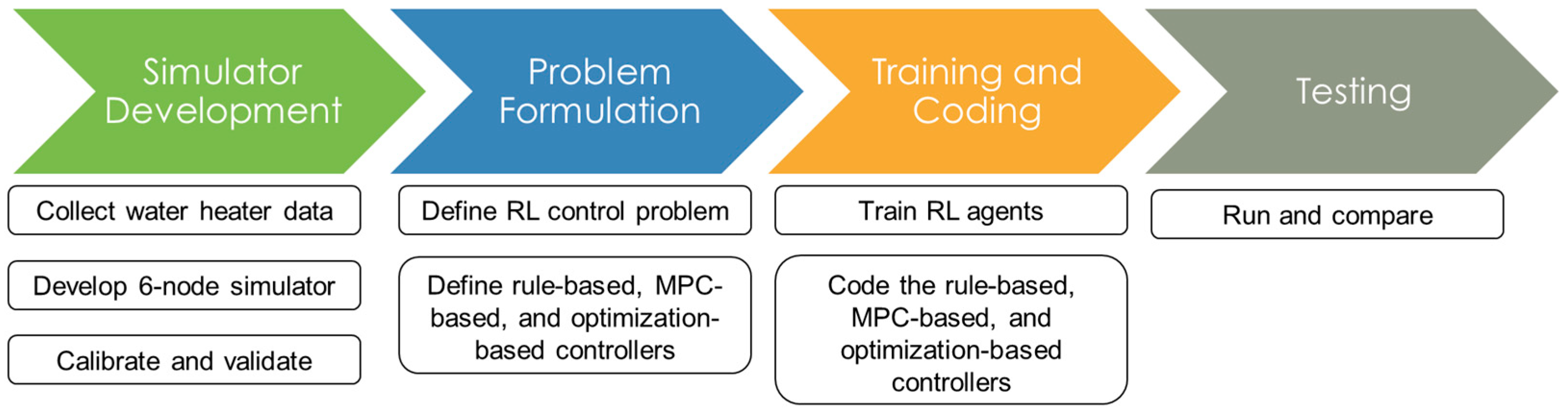
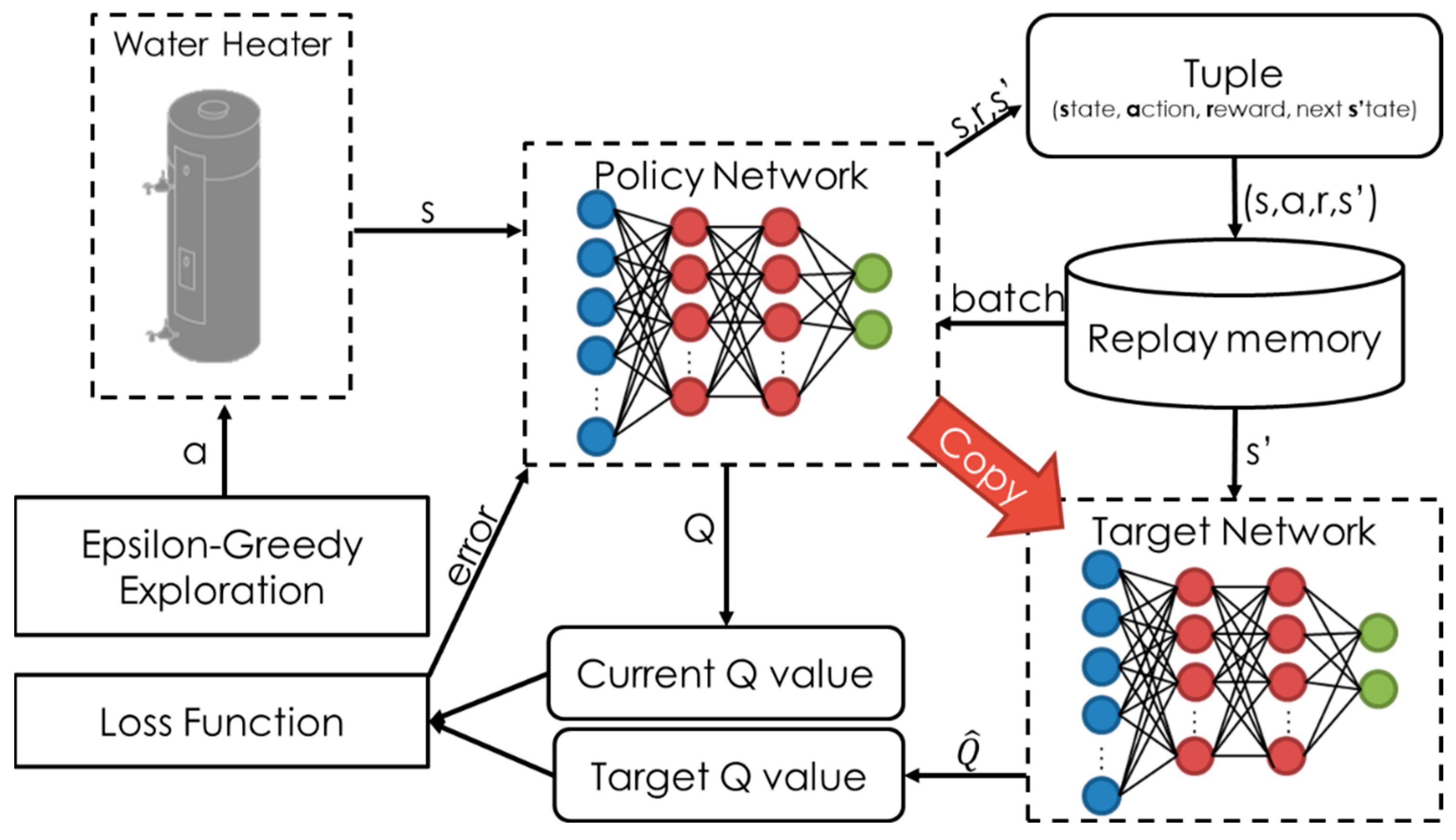
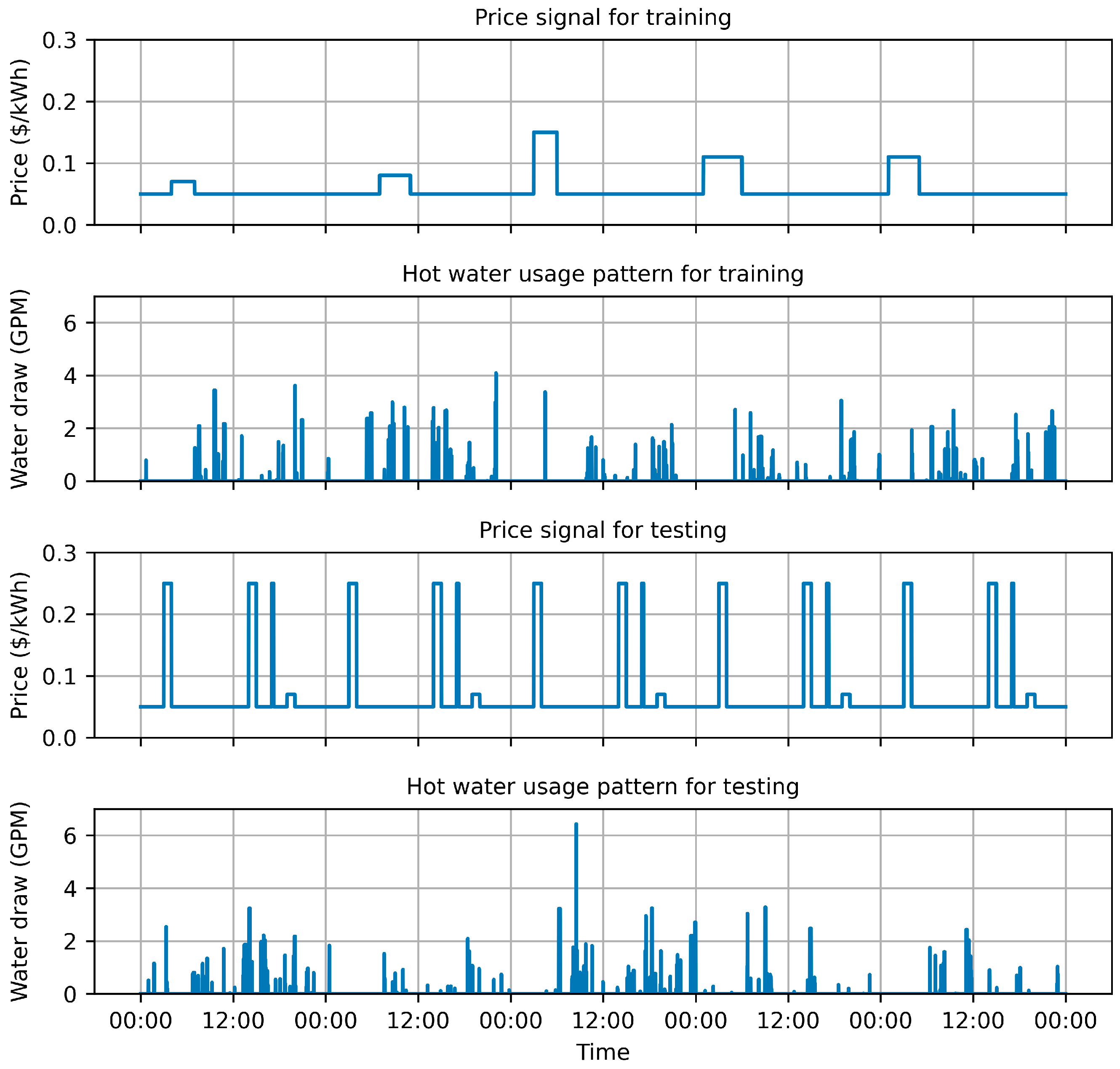
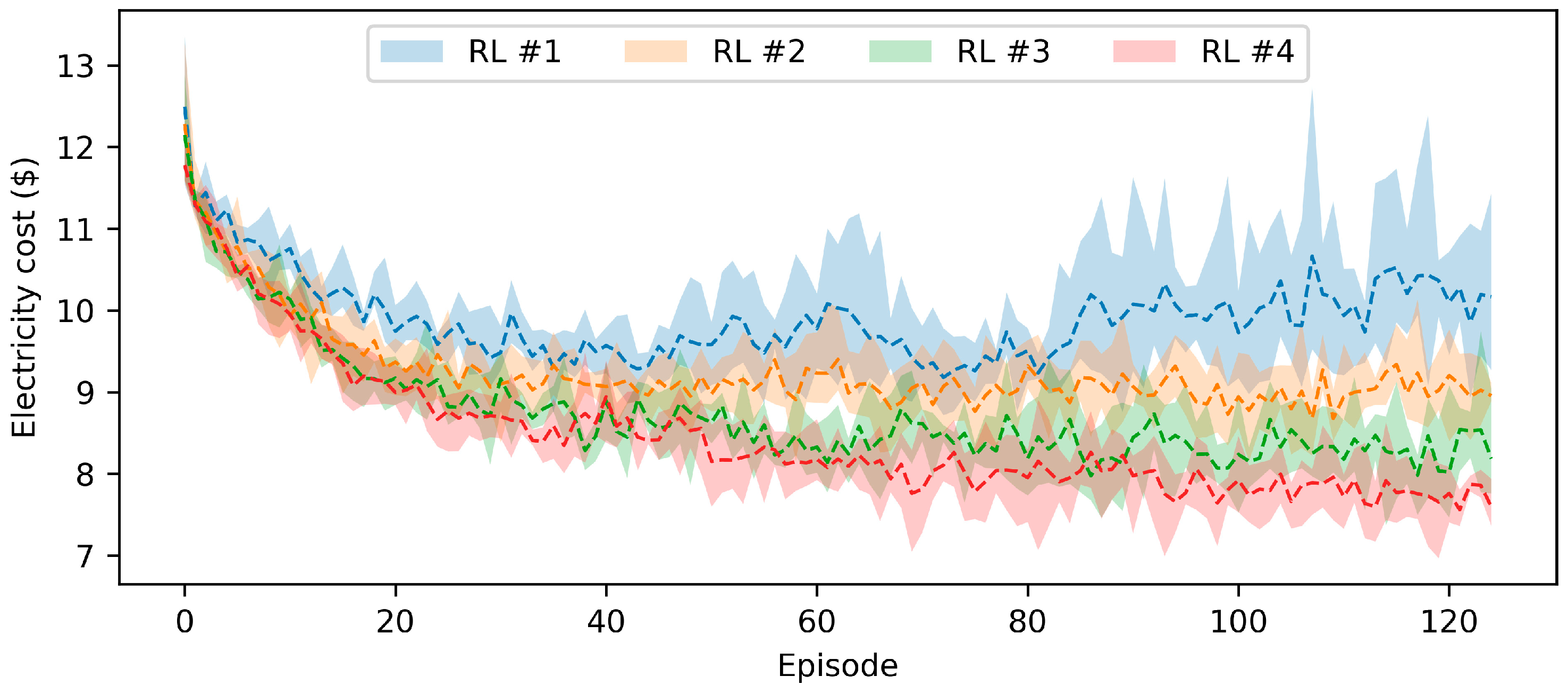
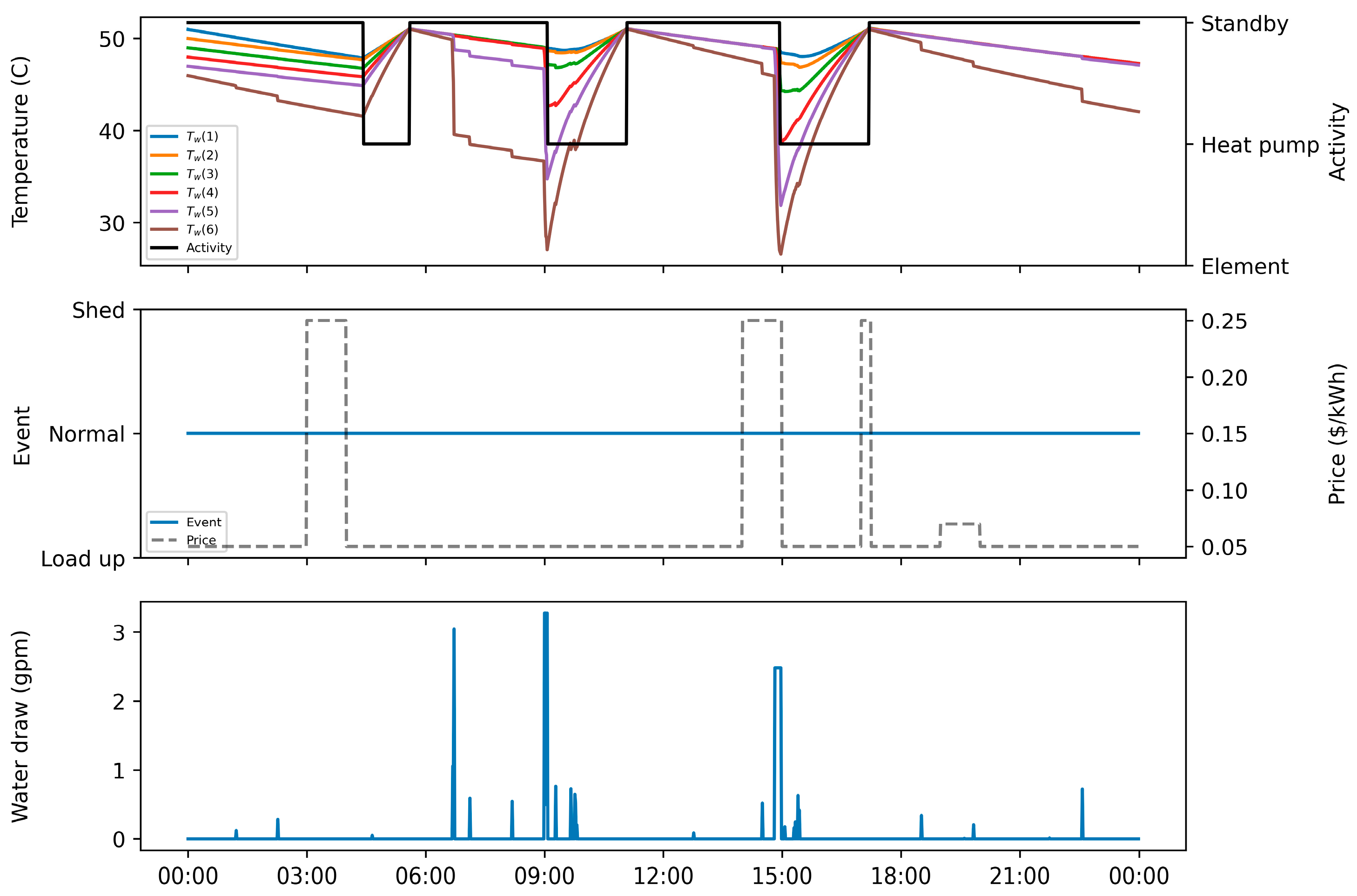
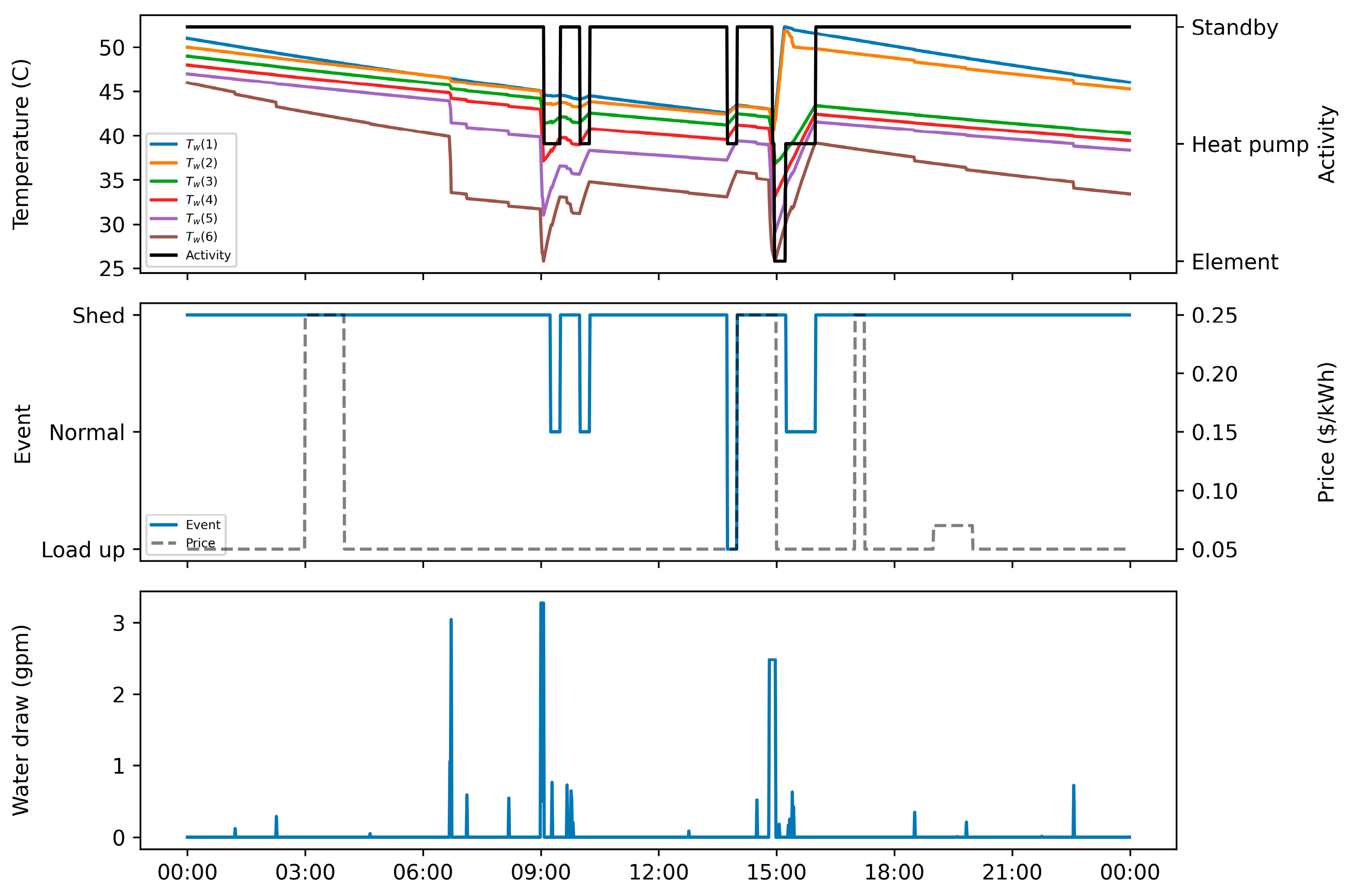
Towards addressing these research gaps, this study proposes a model-free RL approach that aims to minimize the electricity cost of a HPWH under a TOU electricity pricing policy by only using standard DR commands (e.g., shed, load up). In this approach, a set of RL agents, with different look ahead periods, were trained using the deep Q-networks (DQN) algorithm and their performance were tested on an unseen pair of price and hot water usage profiles. Additionally, the RL agents were compared to rule-based, MPC-based, and optimization-based controllers to further validate the performance of the proposed RL approach. This paper contributes to the body of knowledge in two main respects. First, this paper presents a model-free controller for a water heater based on standard DR commands to optimize its operation under TOU electricity pricing policy. Second, this paper compares the performance of the proposed model-free controller against a set of state-of-the-art rule-based, MPC-based and optimization-based controllers.

The paper is structured as follows. Section 2 provides a background about RL, HPWHs and the CTA-2045 standard that the DR commands are based on. Section 3 describes the methodology that was followed to develop the RL agents, the rule-based, the MPC-based, and the optimization-based controllers. Section 4 presents the training and testing results of the RL agents and provides a comparison between the RL agents and other controllers. Finally, Section 5 concludes the paper and discusses the limitations of this study.

2. Background

2.1. Reinforcement Learning

RL is a data-driven approach to understand and automate learning and decision-making aiming towards a goal. Unlike other computational approaches, RL approaches can learn by interacting with its environment and does not require any supervision [30]. The interaction between an RL agent and its environment can be formalized using the formal framework of Markov decision process (MDP). An MDP includes four elements: a set of states $S$, a set of actions $A$, a reward function $r:S\times A$, and transition probabilities between the states $P:S\times A\times S^{\prime }\in \left[0, 1\right]$ [32].

The goal of RL is to find an optimal policy ${\pi }^{\ast }$ that maximizes the expected future reward from time $t: G_t=r_t+\gamma r_{t+1}+{\gamma }^2{r}_{t+2}+\dots ,$ where $0\le \gamma \le 1$ is the discount rate parameter that determines how much to prioritize the future reward. Almost all RL algorithms either estimate a state-value function $V^{\pi }\left(s\right)$ to evaluate how good it is to be in the state $s$ or estimate an action-value function $Q^{\pi }\left(s,a\right)$ to evaluate how good it is to take the action $a$ at the state $s$. The way to achieve this depends on whether the characteristics of the environment are known. On one hand, if the characteristics of the environment are known, approaches such as model-based RL or dynamic programming (DP) can be taken. In these approaches, the RL agent learns or is given the characteristics of the environment, then finds the optimal policy. The use of a state value function $V^{\pi }\left(s\right)$, as defined in Equation (1) is more applicable for model-based approaches [33].

$$V^{\pi }\left(s\right) ={\mathbb{E}}_{\pi }\left[G_t|S_t=s\right] ={\mathbb{E}}_{\pi }\left[{\displaystyle \sum }_{k=0}^{\infty }{\gamma }^k{r}_{t+k}|S_t=s\right]$$

(1)

where $\mathbb{E}$ refers to the expected return (i.e., the discounted cumulative future rewards) of the agent when starting from the state $s$ and following the policy $\pi$.

On the other hand, model-free RL approaches do not need the characteristics of the environment. Such approaches discover an optimal policy by simply interacting with the environment. The use of action-value function $Q^{\pi }\left(s,a\right)$, as defined in Equation (2), is more applicable for model-free approaches [33].

$$Q^{\pi }\left(s,a\right) ={\mathbb{E}}_{\pi }\left[G_t|S_t=s, A_t=s \right] ={\mathbb{E}}_{\pi }\left[{\displaystyle \sum }_{k=0}^{\infty }{\gamma }^k{r}_{t+k}|S_t=s, A_t=a\right]$$

(2)

There are three main model-free RL approaches: policy-based, value-based, and actor–critic, which is a combination of policy- and value-based approaches. The policy-based approaches use optimization techniques and directly search for an optimal policy. In these approaches, the gradient of the objective function is calculated using Equation (3) and then the weight matrix that represents the policy $\theta$ is updated as in Equation (4).

$${\nabla }_{\theta }\mathrm{J}\left(\theta \right) \approx \frac{1}{N} {\displaystyle \sum }_{i=1}^N\left[{\displaystyle \sum }_{t=0}^T{\nabla }_{\theta }log{\pi }_{\theta }\left(a_{i,t}|s_{i,t}\right){\displaystyle \sum }_{t=0}^{T}r\left(s_{i,t},a_{i,t}\right)\right]$$

(3)

$$\theta \leftarrow \theta +\alpha {\nabla }_{\theta }\mathrm{J}\left(\theta \right)$$

(4)

Value-based approaches include SARSA (on-policy) and Q-learning (off-policy), algorithms. These approaches learn the action-value function without explicitly representing the policy function. Both SARSA and Q-learning are tabular approaches and use a look up table (Q-table) to store the values of state-action pairs (Q-values).

The SARSA algorithm evaluates policies by constructing their value functions and uses these value functions to find improved policies [34]. The SARSA algorithm updates the Q-values as follows.

$$Q\left(S_t,A_t\right) \leftarrow Q\left(S_t,A_t\right) + \alpha \left[r_t+\gamma Q\left(S_{t+1},A_{t+1}\right) - Q\left(S_t,A_t\right)\right]$$

(5)

where $\alpha$ refers to the learning rate. As such, the update in Equation (5) is performed after every transition from $S_t$ to $S_{t+1}$, given that $S_{t+1}$ is not a terminal state. If $S_{t+1}$ is the terminal state, then $Q\left(S_{t+1},A_{t+1}\right)$ is defined as zero. This algorithm is called SARSA because it uses $S_t, A_t,R_{t+1}, S_{t+1}, A_{t+1}$.

The Q-learning algorithm begins with a random action-value function and updates to an improved action-value function in an iterative process until reaching the optimal action-value function. The Q-learning algorithm updates the Q-values as follows.

$$Q\left(S_t,A_t\right)\leftarrow Q\left(S_t,A_t\right) + \alpha \left[r_t+\gamma \underset{a}{\max }Q\left(S_{t+1},a\right) - Q\left(S_t,A_t\right)\right]$$

(6)

The value-based approaches can also use deep neural networks (DNN) to estimate the Q-values instead of the Q-table when the size of the combinations of state-action pairs is very high. In such cases, the DNNs represented by $\theta$ are trained to minimize the loss functions. The loss functions for deep SARSA and DQN are given in Equations (7) and (8), respectively.

$$L_i\left({\theta }_i\right) =\mathbb{E}\left[{\left(r_t+\gamma Q\left(S_{t+1},A_{t+1},{\theta }_{i-1}\right) - Q\left(S_t,A_t,{\theta }_i\right)\right)}^2\right]$$

(7)

$$L_i\left({\theta }_i\right) =\mathbb{E}\left[r_t+\gamma \underset{a}{\max }Q\left(S_{t+1},a,{\theta }_{i-1}\right) - Q{\left(S_t,A_t,{\theta }_i\right)}^2\right]$$

(8)

Finally, actor–critic approaches combine value-based and policy-based approaches and use two agents: an actor and a critic. For actor–critic approaches, by replacing the second term with the action-value function (Q-value), Equation (3) can be rewritten as follows:

$${\nabla }_{\theta }\mathrm{J}\left(\theta \right) =\mathbb{E}\left[{\displaystyle \sum }_{t=0}^T{\nabla }_{\theta }log{\pi }_{\theta }\left(a_t|s_t\right)Q_w\left(s_t, a_t\right)\right]$$

(9)

where the critic estimates the action-value function parameterized by $w$ and the actor updates the policy parameters $\theta$.

2.2. Heat Pump Water Heaters

Unlike standard electric water heaters that only include a single or two electric elements to generate heat directly, HPHWs include both a heat pump and electric elements. These water heaters use only the heat pump most of the time and use electric elements as backup during periods of high hot water demand [35]. Because heat pumps move heat from one place to another rather than generating it directly, HPWHs are more efficient than standard electric water heaters [36]. HPWHs can achieve savings more than 50% compared to standard electric water heaters [37].

The overall efficiency of HPWHs depends on two main factors: the use of electric elements and the COP of the heat pump. The higher the use of electric elements, the lower the overall efficiency is. However, operating the water heater with a very narrow deadband to avoid element usage is also not efficient, due to increased losses and higher average heat sink temperatures. Therefore, the lower the water temperature (i.e., heat sink temperature), the higher the heat pump efficiency is. Thus, developing control strategies for HPWHs that maximize heat pump efficiency and minimize the use of relatively inefficient electric elements is critical.

2.3. The CTA-2045 Standard

An efficient control medium is essential to fully harness the flexibility of the demand side. However, the control of the flexible loads is not an easy task, because the DR operators have to coordinate a large number of devices with different manufacturers and communication protocols. To facilitate this, the CTA-2045 standard was established as a universal communication module for gathering data and dispatching commands from/to devices. To date, the CTA-2045 standard has been used for many devices including water heaters, thermostats, electric vehicle chargers, and pool pumps [5].

In the case of water heaters, the CTA-2045 standard enables a water heater with a CTA-2045 communication module to be monitored and controlled remotely. For example, DR operators can monitor the properties (e.g., water heater size and rated power) and operation data (e.g., total and present energy storage capacity) of water heaters and can send several DR commands (e.g., shed and load up) to control water heaters. The use of CTA-2045-compatible water heaters is expected to increase due to the incentives provided to the manufacturers and utilities. For example, it is expected that CTA-2045-enabled water heaters will represent 91% of all water heaters in Washington and Oregon by 2039 [38]. If only 26.5% of these electric water heaters are enrolled for a DR program in these states, 301 MW of demand response potential can be achieved [39]. As the penetration of CTA-2045 grows, it is imperative to develop control strategies that use the DR commands of the CTA-2045 to control water heaters.

3. Methodology

An RL agent can be deployed in an environment to derive an optimal policy through continuously interacting with the environment without any prior knowledge. Although this is feasible for online RL algorithms (e.g., DQN), many researchers have opted to use simulators to train and test the algorithms to avoid the long learning periods and the poor control performance during the learning process [11,40]. Similarly, this study used a simulator for training and testing the RL agents. Figure 1 summarizes the methodology of this study. Accordingly, the research methodology consists of four main steps: (1) developing a CTA-2045-compatible HPWH simulator, (2) formulating the main components (e.g., state, action and reward) of the RL control problem, (3) training the RL agents, (4) developing rule-based, MPC-based, and optimization-based controllers, and (5) performance testing.

3.1. Simulator Development

A 6-node HPWH simulator with two electric elements and a heat pump, adapted from [35,41] was developed. The diagram of the water heater is shown in Figure 2. The 6-node water heater splits the water tank into six equal volumes and assumes that the temperature of each node is homogeneous and the only heat transfer between the nodes is via advection (i.e., bulk motion of the water from one node to another during hot water draws). The simulator calculates the temperature change in each node based on the heat added from the heat pump and/or an element, heat loses through the tank walls, and water draws.

The temperature change in each node ($\Delta T_w\left(N\right))$ at every minute was calculated using the following equation:

$$\Delta T_w\left(N\right) =\frac{{\dot{Q}}_{HP}\times C_{HP}\left(N\right) + {\dot{Q}}_E\times C_E\left(N\right) - UA\left(N\right) \times \left(T_w\left(N\right) - T_{amb}\right) + \dot{m}\times c_p\times \left(T_w\left(N+1\right) - T_w\left(N\right)\right)}{c_p\times m\left(N\right) \times \beta }$$

(10)

where ${\dot{Q}}_{HP}$ and ${\dot{Q}}_E$ are the heats added by the heat pump and an element, respectively, $C_{HP}\left(N\right)$ and $C_E\left(N\right)$ are the fractions of the heat added to node $N$ by the heat pump and element, respectively (Equation (11)), $UA\left(N\right)$ is the standby heat loss coefficient of node $N$, $T_w\left(N\right)$ is the water temperature of node $N$, $T_{amb}$ is the ambient temperature of the room where the water heater is located, $\dot{m}$ is the mass flow rate, $c_p$ is the specific heat of water, $T_w\left(N+1\right)$ is the water temperature of node $N+1$, $m\left(N\right)$ is the mass of water in node $N$, and $\beta$ is a coefficient to take the mass of the water tank wall into account.

Hot water is drawn from the uppermost node and the water heater is filled with fresh water entering at the lowermost nodes. For example, as the water heater is drawn down, node 2 goes up to node 1, node 3 goes up to node 2 and so on. Finally, node 6 (the bottom node) is filled with the fresh water. For this reason, when calculating $\Delta T_w\left(6\right)$, $T_w\left(7\right)$ is taken as the temperature of the fresh inlet water ($T_{inlet}$), because there is no node 7 and node 6 (the bottom node) is filled with the fresh water as the water heater is drawn hot water.

$$\begin{gathered} C_{HP}\left(N\right) =\frac{1}{1+e^{\frac{T_w\left(N\right)-T_w\left(6\right)}{s}-5}}\times {\left(T_{set}-T_w\left(N\right)\right)}^p \forall N \\ {C}_E\left(N\right) =0 \forall N\left(N\ne 2 \wedge N\ne 5\right) \\ {C}_E\left(N\right) =1 \Rightarrow \left(N=2 \vee N=5\right) \end{gathered}$$

(11)

where $s$ is the perceived distance between the lower and upper tank, $T_{set}$ is the temperature setpoint, and $p$ is a parameter to tune the concavity of $T_w\left(N\right)$ reaching the setpoint.

The heat added to the tank by the heat pump (${\dot{Q}}_{HP}$) or an element (${\dot{Q}}_E$) and the resulting electricity consumption ($E_{WH}$) in a minute are calculated using the following equations.

$${\dot{Q}}_{HP}=\frac{P_{HP}\times {\mathrm{COP}}_{HP}\times u_{HP}}{60}$$

(12)

$${\dot{Q}}_E=\frac{P_E\times {\mathrm{COP}}_E\times u_E}{60}$$

(13)

$${\dot{Q}}_E=\frac{P_E\times {\mathrm{COP}}_E\times u_E}{60}$$

(14)

where $P_{HP}$ and $P_E$ are the rated powers, ${\mathrm{COP}}_{HP}$ and ${\mathrm{COP}}_E$ are the coefficients of performance, ${\mathrm{u}}_{HP}$ and ${\mathrm{u}}_E$ are the status (on/off) of the heat pump and an element, respectively. The water heater uses a deadband control logic which uses the weighted average of the temperatures of node 2 and node 5 (Equation (15)). When there is no DR command, the deadbands for the heat pump and the upper element are 5 °C and 10 °C, respectively. For example, if the weighted average drops 5 °C below the setpoint, the heat pump is turned on to heat the water back to the setpoint. If the temperature of node 2 drops 10 °C below the setpoint, first the upper element is turned on to heat the water back to the 4 °C below the setpoint, and then the upper element is turned off and lower element is turned on to heat the water back to the setpoint. The upper and lower elements cannot be on at the same time. However, whenever any element is turned on, the heat pump is also automatically turned on. The DR commands can either increase or decrease the deadband for the heat pump but cannot change the control logic described above.

$$T_{w_{av}}=0.75\times T_w\left(2\right) + 0.25\times T_w\left(5\right)$$

(15)

3.2. Reinforcement Learning Problem Formulation

Four RL agents were formulated. In formulating these RL agents, four different state variable configurations were considered, but the action space and the reward function of the four agents were kept identical. To develop the proposed agents, it was assumed that a CTA-2045-compatible water heater (or simulator) for gathering data and dispatching commands from/to the water heater, and information about electricity prices and hot water usage volumes are available. The data to gather from the water heater includes node temperatures, state of the heat pump and elements, and electricity consumption. Such data are available via a cloud interface (e.g., Skycentrics [42]) for CTA-2045-compatible water heaters. The commands to dispatch include shed, normal, and load up. Similarly, these commands can be dispatched via cloud interface for CTA-2045-compatible water heaters. The electricity prices are available on a day-ahead basis. However, future hot water usage volumes may not be readily available but can be forecasted. Considering this fact, an RL agent that does not use hot water usage volumes was also formulated.

The potential state variables included 25 variables: current temperatures of all nodes ($T_w{\left(1\right)}_t,\dots T_w{\left(6\right)}_t$), electricity prices with 15-min interval averages [$mean\left({\lambda }_{t:t+15}\right), \dots ,mean({\lambda }_{t+7\times 15:t+8\times 15})]$, hot water usage volumes with 15-min interval averages [($mean(V_{t:t+15}),\dots ,mean(V_{t+7\times 15:t+8\times 15})]$, and binary variables to indicate whether the heat pump ($s{1}_t$), the lower element ($s{2}_t$), and the upper element ($s{3}_t$) is on cycle. RL agent #1 did not use the electricity prices of next 30 min but does not use future hot water usage volumes by considering the fact that future volumes may not be known beforehand. Thus, the state variables for RL agent #1 included 11 variables. RL agents #2, #3 and #4, on the other hand, used the water usage volumes and electricity prices of next 30 min, next hour, and next two hours, respectively. Consequently, their state variables included 13, 17 and 25 variables, respectively.

Table 1. State variables of the RL agents.

RL Agent #	State Variables
1	$T_w{\left(1\right)}_t,\dots T_w{\left(6\right)}_t$, $s{1}_t$, $s{2}_t$, $s{3}_t$, $mean({\lambda }_{t:t+15}),mean({\lambda }_{t+15:t+2\times 15})$
2	$T_w{\left(1\right)}_t,\dots T_w{\left(6\right)}_t$, $s{1}_t$, $s{2}_t$, $s{3}_t$, $mean({\lambda }_{t:t+15}),mean({\lambda }_{t+15:t+2\times 15})$, $mean(V_{t:t+15}),mean(V_{t+15:t+2\times 15})$
3	$T_w{\left(1\right)}_t,\dots T_w{\left(6\right)}_t$, $s{1}_t$, $s{2}_t$, $s{3}_t$, $mean({\lambda }_{t:t+15}),\dots ,mean({\lambda }_{t+5\times 15:t+6\times 15})$, $mean\left(V_{t:t+15}\right), \dots ,mean(V_{t+5\times 15:t+6\times 15})$
4	$T_w{\left(1\right)}_t,\dots T_w{\left(6\right)}_t$, $s{1}_t$, $s{2}_t$, $s{3}_t$, $mean({\lambda }_{t:t+15}),\dots ,mean({\lambda }_{t+7\times 15:t+8\times 15})$, $mean\left(V_{t:t+15}\right), \dots ,mean(V_{t+7\times 15:t+8\times 15})$

$T_w{\left(N\right)}_t$: water temperature of node $N$ at time $t$, $s{1}_t$: heat pump status at time $t$, $s{2}_t$: lower element status at time $t$, $s{3}_t$: upper element status at time $t$, ${\lambda }_t$: electricity price at time $t$, $V_t$: hot water usage volume at time $t$.

summarizes the state variables of all RL agents.

The action space for all RL agents included three standard DR commands: shed, normal, and load up. Shed is a curtailment event that increases the deadband for the heat pump to 10 °C. Under shed command, the heat pump turns on when the weighted average given in Equation (15) drops 10 °C below the setpoint to heat up the water back to the setpoint. Load up command, on the other hand, forces the water heater to heat up to the setpoint temperature by reducing the deadband for the heat pump. Under the load up command, the heat pump turns on when the weighted average drops 1 °C below the setpoint to heat up the water back to the setpoint. Normal command cancels any existing DR command and run the water heater with the default deadband for the heat pump.

Finally, the reward ($r_t$) that the agents receive after taking an action at each control time step is given in Equation (16). The reward function only includes a term about electricity cost and does not include any term about comfort due to two reasons. First, user comfort is already maintained because the actions do not change the water temperature setpoint set by users. Second, the upper nodes are reserved for end users by the manufacturer and are not available for any DR command. Regardless of the received DR command, the water heater control logic guarantees the availability of hot water by heating the water in upper nodes when needed.

$$r_t=-c_t=-E_{W{H}_{t:t+15}}\times {\lambda }_{t:t+15}^{\prime }$$

(16)

where $c_t$ is the electricity cost calculated by multiplying the electricity consumed in previous control time step ($E_{W{H}_{t:t+15}}$) by the electricity price in previous control time step (${\lambda }_{t:t+15}$).

3.3. Reinforcement Learning Training

For training the RL agents, the DQN algorithm (Figure 3) was used. The DQN algorithm, presented in Algorithm 1, has two important ingredients. First, the DQN algorithm includes two networks: policy network ($\theta$) and target network ($\widehat{\theta }$). The policy network is constantly updated and determines the actions to take while interacting with the environment. The target network is updated by taking the weights from the policy network at regular intervals and predicts the Q-value of the next state. Second, the DQN algorithm includes a replay memory to store previous experiences. The policy network updates its weights, using a random batch (of experiences) taken from the replay memory. The replay memory helps with breaking the correlation between consecutive observations [40]. The algorithm uses the following loss function:

$$L_i\left({\theta }_i\right) =\mathbb{E}\left[{\left(r_t+\gamma \underset{a}{\max }Q\left(S_{t+1},a,\widehat{\theta }\right)- Q\left(S_t,A_t,{\theta }_i\right)\right)}^2\right]$$

(17)

Algorithm 1 DQN training

Initialize replay memory with capacity of N

Initialize policy network with random weights

Initialize the counter: $\xi =0$

for $episode=1,M$ do

Get the initial state $s_t$

Copy the weights of policy network to target network at every $K$ episode

for $t=1,dt,T$ do

Scale state values between [0, 1]         Update the value of $\epsilon$: $\epsilon ={\epsilon }_{end}+ \left({\epsilon }_{start}-{\epsilon }_{end}\right) \times e^{-\xi /{\epsilon }_{decay}}$

Select a random action $a_t$ with probability of $\epsilon$

Otherwise select action $a_t$, using the policy network

Execute action $a_t$ in the water heater model

Observe reward $r_t$ and next state $s_{t+1}$

Store transitions $\left(s_t, a_t, r_t, s_{t+1}\right)$ in replay memory

Move to next state: $s_t:=s_{t+1}$

Sample a batch of transitions $\left(s,a,r,s^{\prime }\right)$ from replay memory

Calculate state action values $Q\left(s,a,\theta \right)$ using the policy network

Calculate the expected state action values $y=\left\{\begin{array}{c}r for terminal\\ r+\gamma ma{x}_{a^{\prime }}Q\left(s^{\prime },a^{\prime },\widehat{\theta }\right) for non terminal\end{array}\right.$

Calculate the loss between the calculated $Q\left(s,a,\theta \right)$ and $y$ values using Equation (17)

Perform a gradient descent and update the weights of $\theta$

Update the counter: $\xi :=\xi +1$

end

end

3.4. Rule-Based, MPC-Based, and Optimzation-Based Controllers

To better evaluate the performance of the proposed RL approach, rule-based, MPC-based and optimization-based controllers were also developed as benchmarks. The rule-based controller followed the logic provided in Algorithm 2. This controller sends load up to heat up the water when the price is low and there is an upcoming water draw; sends normal when the price is low and there is no upcoming water draw; and sends shed in other cases to operate the water heater in lower temperatures for higher COP values.

Algorithm 2 Rule-based controller

for $t=1,dt,T$ do

if $\mathrm{mean}\left({\lambda }_{t:t+dt}\right) <\mathrm{mean}\left({\lambda }_{1:T}\right)$ and $\mathrm{sum}\left(V_{t:t+dt}\right) >0$ then

send Load up

else if $\mathrm{mean}\left({\lambda }_{t:t+dt}\right) <\mathrm{mean}\left({\lambda }_{1:T}\right)$ and $\mathrm{sum}\left(V_{t:t+dt}\right) =0$ then

send Normal

else

send Shed

For fairness of comparison, the MPC-based controllers used the same prediction and control horizons as the RL agents. Accordingly, MPC-based controllers with three different prediction horizons were developed: MPC with 30 min, an hour, and two hours prediction horizons. Additionally, for all MPC-based controllers, the control horizon of 15 min, same as the RL agents, was implemented. The MPC-based controllers are based on three main steps. First, the controller gets the temperatures of all nodes from the simulator and collects the electricity price and hot water usage volumes for the corresponding prediction horizon. Second, the control variables are optimized by genetic algorithm (GA) for the prediction horizon for a minimum electricity cost. The optimization problem was solved using GA because the water heater simulator is nonlinear and non-convex. For nonlinear models, global search metaheuristic methods such as GA, can achieve near-optimal solutions with a certain probability, which is useful to solve the optimization problems with complicated scenarios [30,31]. Third, the optimal control variables resulting from the optimization were implemented for the control horizon.

For the optimization-based controller, the control variables were optimized for the entire simulation period using GA. This controller assumes that perfect information about the future is available. For example, it assumes that a day-ahead hot water usage volume is available with perfect accuracy. Therefore, this controller may not be applicable for real problems. However, in this study it was implemented only for the sake of creating a golden standard. Both MPC-based and optimization-based controllers were developed using Python on a standard four-core personal computer.

3.5. Performance Testing

The performance testing included two comparisons. First, the resulting RL agents were compared against a baseline that was established by running the simulator without sending any DR commands. As such, the resulting RL agents were deployed on the simulator for 30 days. For these 30 days, the simulator was provided with hot water usage and price profiles different from the ones used in the training stage. The testing of the RL agents was performed in an offline manner. The RL agents were not further trained during the testing. Second, the performance of the RL agents were compared against the rule-based, MPC-based, and optimization-based controllers for five days. The comparison between RL agents and other controllers was conducted for five days because the MPC-based controllers require an optimization in each control time step. Thus, longer simulation periods result in longer computational times. Additionally, because the optimization-based controller optimizes the operation for the entire simulation period, longer simulation periods would result in more variables, which makes the optimization more challenging.

4. Experiments and Results

4.1. Water Heater Experiments and Simulator Results

To ensure the water heater simulator was realistic and represents the behavior of an actual water heater, a set of experiments with an actual 250-L HPHW was conducted to determine the parameters of the simulator. As such, the water heater was instrumented with three thermistors, an ambient temperature sensor, a power meter, and a flow meter.

Table 2. Measurement devices.

Instrument Type	Instrument Name	Error Range
Thermistor	Omega 44031 10 kOhm Precision	±0.01 °C
Ambient temperature sensor	Campbell Scientific HC2S3	±0.01 °C
Power meter	WattNode Pulse	±0.5%
Flow meter	Omega FTB4607	±2.0%

summarizes the instruments and their error ranges. The following data were collected from the water heater in minute intervals: inlet water temperature (°C), outlet water temperature (°C), ambient air temperature (°C), lower tank water temperature (°C), upper tank water temperature (°C), hot waterflow (GPM), and electricity demand (W). The resulting dataset was split into training and testing datasets. Using the training dataset, four analyses were performed. First, the values of water mass in a node and specific heat of water were set using common knowledge. Second, parameters including ambient temperature, inlet water temperature, temperature setpoint, heat pump rated power, and element rated power were assumed constant and were set by averaging their values in the training dataset. Third, the COPs of the heat pump and elements were calculated. Finally, the remaining unknown parameters (e.g., $UA, p$) were optimized in a way that minimizes the sum of the root mean squared error (RMSE) of lower and upper temperatures.

Table 3. Parameters of the water heater simulator.

Parameter	Explanation	Value	Unit
$c_p$	Specific heat of water	4.184	$\mathrm{J}/\left(\mathrm{g}·\mathrm{K}\right)$
$m\left(N\right)$	Water mass in a node	41.7	kg
$T_{amb}$	Ambient temperature	21.5	°C
$T_{inlet}$	Inlet water temperature	23.9	°C
$T_{set}$	Temperature setpoint	51	°C
$P_{HP}$	Heat pump rated power	400	$\mathrm{W}$
$P_E$	Element rated power	4500	$\mathrm{W}$
COPHP	COP of heat pump	$-0.004\times T_w{\left(5\right)}^{2}0.19\times T_w\left(5\right) + 3.56$	N/A
COPE	COP of element	0.99	N/A
$UA\left(1\right)\dots UA\left(6\right)$	Standby heat loss coefficients	0.04, 0.03, 0.03, 0.03, 0.03, 0.06	$\mathrm{kJ}/\left(\min ·\mathrm{K}\right)$
$\beta$	Water tank wall coefficient	1.12	N/A
$s$	Perceived distance	3.7	N/A
$p$	Concavity parameter	1.06	N/A

shows the resulting parameters of the water heater simulator.

Then, the simulator was validated using the testing dataset. The simulator was run with the same conditions as the actual water heater. Then, the measurements from the actual and the simulated water heaters were compared. Figure 4 shows the accuracy of the simulator in predicting upper and lower temperatures and power consumption level for a randomly selected day. As shown, the simulator was pretty accurate. It achieved RMSEs of 1.13 °C and 1.34 °C for lower and upper tank temperatures, respectively. Overall, these results showed that the water heater simulator is realistic and therefore capable of representing the behavior of an actual water heater.

4.2. Price and Hot Water Usage Profiles

Separate pairs of price and water usage profiles were used for training and testing the RL agents. In training the RL agents, a typical TOU price signal, consisting of 3 h peak and 21 h off-peak prices per day, was used. The peak price period in TOU price signal was determined randomly for every day. In testing the RL agents, a price signal, consisting of two peaks, a mid-peak, and an off peak, was used to better verify the adaptability of the RL agents to different price signals. For hot water usage profiles, the domestic hot water (DHW) event schedule generator tool provided by the U.S. Department of Energy (DOE) was used [43]. The RL agents were trained on June and July usage profiles and tested on August profile. Figure 5 shows a sample from the price and hot water usage profiles for training and testing.

4.3. Training Results

All RL agents were trained based on Algorithm 1 using Python with the PyTorch framework [44] on a standard four-core personal computer with parameters as summarized in

Table 4. Hyperparameters of the RL agent training.

Parameter	Explanation
Batch size	32
Discount rate ($\gamma$)	0.99
${\epsilon }_{start}$	0.5
${\epsilon }_{end}$	0.03
${\epsilon }_{decay}$	140,000
Target network update frequency ($K$)	Every episode
Number of episodes ($M$)	125
Episode length ($T$)	61 days
Replay memory capacity ($N$)	25,000
DNN structure	[L,512,512,3] 1
DNN optimizer	RMSprop
Optimizer learning rate	0.0001
DNN loss function	Mean squared error (MSE)
Control time step ($dt$)	15 min

¹ L is the number of state variables.

. The training of each RL agent was repeated five times. Figure 6 shows the average, maximum, and minimum operation costs of the RL agents per episode. The RL agents reduced the electricity cost per episode as the training advances. Despite all RL agents being able to reduce the electricity cost significantly, the RL agents with more future state variables have achieved more savings in training data. For example, the RL agent #4 was able to reduce the average electricity cost to USD 7.59 while the RL agent #1 could reduce it to USD 10.17. On average, one episode took 3 min to be simulated on a machine with an Intel Xeon CPU @ 3.70 GHz processor and 16.0 GB RAM.

4.4. Testing Restuls

Table 5. Comparison of baseline and RL.

Operation Strategy	Look Ahead	Electricity Cost	Element Usage	Average COPHP
Baseline	N/A	USD 6.04	121 min	4.79
RL agent #1	30 min *	USD 5.03	226 min	5.30
RL agent #2	30 min	USD 4.37	106 min	5.39
RL agent #3	1 h	USD 3.55	73 min	5.47
RL agent #4	2 h	USD 3.44	71 min	5.58

* future price information only.

shows the electricity costs, element usages, and average COPs of the baseline and the RL agents over 30 days. All RL agents were able to achieve significant cost savings over the baseline over this period. The operation cost of the baseline was USD 6.04. Figure 7 shows the operation of the baseline model on a randomly selected day. RL agents #1, #2, #3 and #4 were able to reduce the cost of the water heater operation to USD 5.03, USD 4.37, USD 3.55 and USD 3.44, respectively, over the same period. Additionally, in all cases the temperature of the hot water drawn was never less than the 10 °C below the setpoint, which shows that comfort of end users were maintained.

The RL agents were able to reduce the electricity cost of the water heater for two main reasons. First, all RL agents could successfully avoid peak price periods and run the heat pump and/or an element during off price periods whenever it is possible. For example, the RL agent #4 turned on the heat pump for 8945 min and only 305 min of these were during peak price. However, the baseline turned on the heat pump for 12,366 min and 1765 min of these were during peak price. For RL agent #4, only 3.41% of the heat pump operation coincided with peak price periods, whereas 14.27% for the baseline. Second, RL agents #2, #3 and #4 could maintain a good balance between the use of heat pump and relatively inefficient electric elements. As a result, these RL agents achieved higher COP_HP values and less element usages. For example, the RL agent #2 used elements for 106 min and had the average COP_HP of 5.39, whereas the baseline used elements for 121 min and had the average COP_HP of 4.79. RL agent #1, however, was not able to reduce the element usage because it could not do any preheating prior to large hot water draws since it does not have any information about future hot water draws. Figure 8 shows the operation of RL agent #1 on a sample day. As shown in the figure, the agent only sent normal and load up commands when the price was low and was able to avoid higher price periods. For example, the agent heated up the water by sending load up commands before and after the peak price around 15:00. Consequently, the agent could avoid peak price periods. In addition, the agent sent shed commands most of the time to operate in lower temperatures for higher COP values. However, unlike RL agent #1, did not do any heating before or after peak price periods and therefore could not avoid the peak price at 17:00.

Table 6. Performance of RL agents, and MPC-based and optimization-based controllers.

Operation Strategy	Look Ahead	Electricity Cost	Element Usage	Average COPHP
Baseline	N/A	USD 1.36	75 min	4.88
Rule-based	N/A	USD 1.10	58 min	4.63
RL agent #2	30 min	USD 1.10	68 min	5.35
RL agent #3	1 h	USD 0.89	58 min	5.27
RL agent #4	2 h	USD 0.88	54 min	5.47
MPC #2	30 min	USD 1.31	157 min	5.76
MPC #3	1 h	USD 1.04	104 min	5.70
MPC #4	2 h	USD 0.94	84 min	5.61
Optimization	5 days	USD 0.81	47 min	5.48

summarizes the performance of the RL agents, the rule-based, MPC-based, and optimization-based controllers over five days. The rule-based controller achieved 19.1% savings. RL agents #2, #3 and #4 achieved 19.1%, 34.6% and 35.3% savings, respectively, whereas their counterparts, MPC #2, MPC #3 and MPC #4, achieved 3.7%, 23.5% and 30.9% savings, respectively. The optimization-based controller, as the golden standard, achieved a 40.4% saving.

Overall, all controllers achieved significant savings compared to baseline. The rule-based controller, despite its very simple structure, was able to perform better than MPC #2. In terms of element usage, it performed very closely to RL agent #4 and the optimization-based controller, but could not maintain a good balance between element usage and COP_HP, and therefore got the lowest COP_HP values. The rule-based controller simply operated the water heater in high temperatures to minimize the use of elements at the expense of low heat pump efficiency. The RL agents outperformed their corresponding MPC controllers for all look ahead periods including 30 min, 1 h and 2 h. For example, the RL agent with 2 h of future hot water usage volumes and electricity prices information (RL agent #4) achieved USD 0.88, while MPC #4 achieved USD 0.94 using the same information. Figure 9 and Figure 10 show the operations based on RL agent #4 and MPC #4, respectively. Overall, the RL agents maintained a good balance between element usage and COP_HP. The MPC-based controllers achieved the highest COP_HP values, which however increased their element use. For example, RL agent #4 had an average COP_HP of 5.47, while MPC #4, the equivalent of RL agent #4, had an average COP_HP of 5.61. RL agent #4 used elements for 54 min only while MPC #4 used elements for 84 min. As a result, despite very close performance, RL agent #4 cost 6¢ less than MPC #4 in five days due to less element usage. The cost of RL agent #4 was also very close to the cost of the optimization-based controller. These results, therefore, show that RL is able to reduce electricity cost without any prior knowledge about the water heater and its power usage. RL can also adapt to unseen price signal and water usage profiles.

In practice, this research can empower multiple stakeholders, including utilities and building occupants. Because the proposed approach is easily scalable and uses the standard DR commands only, utilities can easily adapt this RL approach to their DR programs to control participating water heaters. For example, utilities can use such approaches to minimize electricity consumption during peak periods or to maximize the consumption of renewable energy. Given that the use of the CTA-2045-compatible water heaters is expected to increase due to the incentives provided to the manufacturers, there is a tremendous potential for such approaches to have an application area in utility side. Additionally, these results showed that RL can reduce the cost of the water heater operation more than 30%. Therefore, this research has an application area for the development of BEMS to save building occupants electricity cost. In the context of BEMS, similar RL approaches can also be used for other devises such as HVAC and energy storage units.

5. Conclusions and Limitations

This paper presented an RL-based water heater control approach that aims to minimize the electricity cost of a water heater under a TOU electricity pricing policy. A set of RL agents were trained using the DQN algorithm and their performance was tested on an unseen pair of price and hot water usage profiles for 30 days. In addition, the performance of the developed RL agents was further validated through comparison to a set of rule-based, MPC-based and optimization-based controllers for five days. The comparison between RL agents and other controllers was conducted for five days because the MPC-based controllers require an optimization in each control time step. Thus, longer simulation periods result in longer computational times. Additionally, because the optimization-based controller optimizes the operation for the entire simulation period, longer simulation periods would result in more variables, which makes the optimization more challenging.

The results showed that the proposed approach can help save electricity cost significantly without any prior knowledge about the device. The RL agents were able to outperform the rule-based and MPC-based controllers and saved electricity cost in the range of 19% to 35% compared to the baseline operation. Additionally, the RL agent with 2 h of future hot water usage volumes and electricity prices information (RL agent #4) achieved a very close performance to the golden standard (i.e., the optimization-based controller).

Two main limitations are acknowledged. First, the proposed approach was tested on a water heater simulator. Although the simulator used in this study was validated using an actual water heater, the results and outcomes of this study are still based on a simulator. Additional field studies, therefore, need to be conducted in future work to see if/how the experimental results and findings—in terms of cost saving performance and comparison between RL and MPC—will change for actual water heaters. Second, for all MPC-based and optimization-based controllers, and RL agents #2, #3 and #4, it was assumed that future hot water usage volumes are known. However, future hot water usage volumes may not be known. Future research efforts could study the forecasting of future hot water usage volumes. In addition, additional experiments can be conducted to explore whether hot water usage patterns can be represented by a set of proxy variables (e.g., time of day).

References

1. International Energy Agency. Renewables 2019; International Energy Agency: Paris, France, 2019. [Google Scholar]
2. Enerdata. Global Energy Statistical Yearbook 2020. Available online: https://yearbook.enerdata.net/renewables/renewable-in-electricity-production-share.html (accessed on 3 December 2020).
3. Jensen, S.Ø.; Marszal-Pomianowska, A.; Lollini, R.; Pasut, W.; Knotzer, A.; Engelmann, P.; Stafford, A.; Reynders, G. IEA EBC Annex 67 energy flexible buildings. Energy Build. 2017, 155, 25–34. [Google Scholar] [CrossRef] [Green Version]
4. Department of Energy. Demand Response. Available online: https://www.energy.gov/oe/activities/technology-development/grid-modernization-and-smart-grid/demand-response (accessed on 14 December 2020).
5. National Rural Electric Cooperative Association. Standardized Communications for Demand Response; National Rural Electric Cooperative Association: Arlington, VA, USA, 2018. [Google Scholar]
6. Ruelens, F.; Claessens, B.J.; Quaiyum, S.; Schutter, B.D.; Babuška, R.; Belmans, R. Reinforcement learning applied to an electric water heater: From theory to practice. IEEE Trans. Smart Grid 2018, 9, 3792–3800. [Google Scholar] [CrossRef] [Green Version]
7. Energy Information Administration. Annual Energy Outlook 2020 with Projections to 2050; U.S. Energy Information Administration: Washington, DC, USA, 2020.
8. Energy Information Administration. 2015 Residential Energy Consumption Survey; Energy Information Administration: Washington, DC, USA, 2015.
9. Department of Energy. New Infographic and Projects to Keep Your Energy Bills out of Hot Water. Available online: https://www.energy.gov/articles/new-infographic-and-projects-keep-your-energy-bills-out-hot-water (accessed on 14 December 2020).
10. Wang, F.; Kusnandar; Lin, H.; Tsai, M. Energy Efficient Approaches by Retrofitting Heat Pumps Water Heating System for a University Dormitory. Buildings 2021, 11, 356. [Google Scholar] [CrossRef]
11. Wang, Z.; Hong, T. Reinforcement learning for building controls: The opportunities and challenges. Appl. Energy 2020, 269, 115036. [Google Scholar] [CrossRef]
12. Vanthournout, K.; Hulst, R.D.; Geysen, D.; Jacobs, G. A Smart Domestic Hot Water Buffer. IEEE Trans. Smart Grid 2012, 3, 2121–2127. [Google Scholar] [CrossRef]
13. Péan, T.Q.; Ortiz, J.; Salom, J. Impact of Demand-Side Management on Thermal Comfort and Energy Costs in a Residential nZEB. Buildings 2017, 7, 37. [Google Scholar] [CrossRef] [Green Version]
14. Perera, D.W.; Skeie, N.-O. Comparison of Space Heating Energy Consumption of Residential Buildings Based on Traditional and Model-Based Techniques. Buildings 2017, 7, 27. [Google Scholar] [CrossRef] [Green Version]
15. Manrique Delgado, B.; Ruusu, R.; Hasan, A.; Kilpeläinen, S.; Cao, S.; Sirén, K. Energetic, Cost, and Comfort Performance of a Nearly-Zero Energy Building Including Rule-Based Control of Four Sources of Energy Flexibility. Buildings 2018, 8, 172. [Google Scholar] [CrossRef] [Green Version]
16. Killian, M.; Kozek, M. Ten questions concerning model predictive control for energy efficient buildings. Build. Environ. 2016, 105, 403–412. [Google Scholar] [CrossRef]
17. Perera, A.T.D.; Kamalaruban, P. Applications of reinforcement learning in energy systems. Renew. Sustain. Energy Rev. 2021, 137, 110618. [Google Scholar] [CrossRef]
18. Tarragona, J.; Fernández, C.; de Gracia, A. Model predictive control applied to a heating system with PV panels and thermal energy storage. Energy 2020, 197, 117229. [Google Scholar] [CrossRef]
19. Gholamibozanjani, G.; Tarragona, J.; Gracia, A.d.; Fernández, C.; Cabeza, L.F.; Farid, M. Model predictive control strategy applied to different types of building for space heating. In Thermal Energy Storage with Phase Change Materials; Mohammed Farid, A.A., Gohar, G., Eds.; CRC Press: Boca Raton, FL, USA, 2021; Volume 4.3. [Google Scholar]
20. Starke, M.; Munk, J.; Zandi, H.; Kuruganti, T.; Buckberry, H.; Hall, J.; Leverette, J. Real-Time MPC for Residential Building Water Heater Systems to Support the Electric Grid. In Proceedings of the 2020 IEEE Power & Energy Society Innovative Smart Grid Technologies Conference (ISGT), Washington, DC, USA, 17–20 February 2020; pp. 1–5. [Google Scholar]
21. Wang, J.; Li, C.; Li, P.; Che, Y.; Zhou, Y.; Li, Y. MPC-based interval number optimization for electric water heater scheduling in uncertain environments. Front. Energy 2019. [Google Scholar] [CrossRef]
22. Nazemi, S.D.; Jafari, M.A.; Zaidan, E. An Incentive-Based Optimization Approach for Load Scheduling Problem in Smart Building Communities. Buildings 2021, 11, 237. [Google Scholar] [CrossRef]
23. Görges, D. Relations between Model Predictive Control and Reinforcement Learning. IFAC-PapersOnLine 2017, 50, 4920–4928. [Google Scholar] [CrossRef]
24. Wei, T.; Yanzhi, W.; Zhu, Q. Deep reinforcement learning for building HVAC control. In Proceedings of the 2017 54th ACM/EDAC/IEEE Design Automation Conference (DAC), Austin, TX, USA, 18–22 June 2017; pp. 1–6. [Google Scholar]
25. Kurte, K.; Munk, J.; Kotevska, O.; Amasyali, K.; Smith, R.; McKee, E.; Du, Y.; Cui, B.; Kuruganti, T.; Zandi, H. Evaluating the Adaptability of Reinforcement Learning Based HVAC Control for Residential Houses. Sustainability 2020, 12, 7727. [Google Scholar] [CrossRef]
26. Wang, Y.; Velswamy, K.; Huang, B. A Long-Short Term Memory Recurrent Neural Network Based Reinforcement Learning Controller for Office Heating Ventilation and Air Conditioning Systems. Processes 2017, 5, 46. [Google Scholar] [CrossRef] [Green Version]
27. Kazmi, H.; Mehmood, F.; Lodeweyckx, S.; Driesen, J. Gigawatt-hour scale savings on a budget of zero: Deep reinforcement learning based optimal control of hot water systems. Energy 2018, 144, 159–168. [Google Scholar] [CrossRef] [Green Version]
28. Al-jabery, K.; Wunsch, D.C.; Xiong, J.; Shi, Y. A novel grid load management technique using electric water heaters and Q-learning. In Proceedings of the 2014 IEEE International Conference on Smart Grid Communications (SmartGridComm), Venice, Italy, 3–6 November 2014; pp. 776–781. [Google Scholar]
29. Zsembinszki, G.; Fernández, C.; Vérez, D.; Cabeza, L.F. Deep Learning Optimal Control for a Complex Hybrid Energy Storage System. Buildings 2021, 11, 194. [Google Scholar] [CrossRef]
30. Sutton, R.S.; Barto, A.G. Reinforcement Learning: An Introduction; MIT Press: Cambridge, MA, USA, 2018. [Google Scholar]
31. Mnih, V.; Kavukcuoglu, K.; Silver, D.; Rusu, A.A.; Veness, J.; Bellemare, M.G.; Graves, A.; Riedmiller, M.; Fidjeland, A.K.; Ostrovski, G.; et al. Human-level control through deep reinforcement learning. Nature 2015, 518, 529–533. [Google Scholar] [CrossRef]
32. Vázquez-Canteli, J.R.; Nagy, Z. Reinforcement learning for demand response: A review of algorithms and modeling techniques. Appl. Energy 2019, 235, 1072–1089. [Google Scholar] [CrossRef]
33. Han, M.; May, R.; Zhang, X.; Wang, X.; Pan, S.; Da, Y.; Jin, Y. A novel reinforcement learning method for improving occupant comfort via window opening and closing. Sustain. Cities Soc. 2020, 61, 102247. [Google Scholar] [CrossRef]
34. Han, M.; May, R.; Zhang, X.; Wang, X.; Pan, S.; Yan, D.; Jin, Y.; Xu, L. A review of reinforcement learning methodologies for controlling occupant comfort in buildings. Sustain. Cities Soc. 2019, 51, 101748. [Google Scholar] [CrossRef]
35. Boudreaux, P.R.; Munk, J.D.; Jackson, R.K.; Gehl, A.C.; Parkison, A.E.; Nutaro, J.J. Improving Heat Pump Water Heater Effeciency by Avoiding Electric Resistance Heater Use; Oak Ridge National Laboratory: Oak Ridge, TN, USA, 2014.
36. Hepbasli, A.; Kalinci, Y. A review of heat pump water heating systems. Renew. Sustain. Energy Rev. 2009, 13, 1211–1229. [Google Scholar] [CrossRef]
37. Hudon, K.; Sparn, B.; Christensen, D.; Maguire, J. Heat Pump Water Heater Technology Assessment Based on Laboratory Research and Energy Simulation Models. In Proceedings of the ASHRAE Winter Conference, Chicago, IL, USA, 21–25 January 2012. [Google Scholar]
38. Clarke, T.; Slay, T.; Eustis, C.; Bass, R.B. Aggregation of Residential Water Heaters for Peak Shifting and Frequency Response Services. IEEE Open Access J. Power Energy 2020, 7, 22–30. [Google Scholar] [CrossRef]
39. Bonneville Power Administration. CTA-2045 Water Heater Demonstration Report; Bonneville Power Administration: Portland, OR, USA, 2018.
40. Brandi, S.; Piscitelli, M.S.; Martellacci, M.; Capozzoli, A. Deep reinforcement learning to optimise indoor temperature control and heating energy consumption in buildings. Energy Build. 2020, 224, 110225. [Google Scholar] [CrossRef]
41. Sparn, B.; Hudon, K.; Christensen, D. Laboratory Performance Evaluation of Residential Integrated Heat Pump Water Heaters; National Renewable Energy Laboratory: Golden, CO, USA, 2014.
42. Skycentrics. Available online: https://skycentrics.com/ (accessed on 3 November 2020).
43. Department of Energy. Building America DHW Event Schedule Generator. Available online: https://www.energy.gov/eere/buildings/downloads/building-america-dhw-event-schedule-generator (accessed on 4 February 2020).
44. Paszke, A.; Gross, S.; Massa, F.; Lerer, A.; Bradbury, J.; Chanan, G.; Killeen, T.; Lin, Z.; Gimelshein, N.; Antiga, L. Pytorch: An imperative style, high-performance deep learning library. In Advances in Neural Information Processing Systems 32; Curran Associates, Inc.: Red Hook, NY, USA, 2019; pp. 8026–8037. [Google Scholar]
Figure 1. The framework of the methodology.
Buildings 11 00548 g001
Figure 2. The diagram of the water heater.
Buildings 11 00548 g002
Figure 3. An overview of the DQN algorithm.
Buildings 11 00548 g003
Figure 4. Simulator performance.
Buildings 11 00548 g004
Figure 5. A sample from price and hot water profiles for training and testing.
Buildings 11 00548 g005
Figure 6. Training performance of the RL agents.
Buildings 11 00548 g006
Figure 7. Baseline operation.
Buildings 11 00548 g007
Figure 8. Operation based on RL agent #1.
Buildings 11 00548 g008
Figure 9. Operation based on RL agent #4.
Buildings 11 00548 g009
Figure 10. Operation based on MPC #4.
Buildings 11 00548 g010