A Comprehensive Evaluation Method for Air-Conditioning System Plants Based on Building Performance Simulation and Experiment Information

Abstract

During the design stage of an HVAC (heating, ventilation, and air conditioning) system in a construction project, designers must decide on the most workable design scheme for the plant room in the building based on the evaluation of multiple aspects related to system performance that need to be considered, such as energy efficiency, economic effectiveness, etc. To solve this problem, this paper proposes a comprehensive evaluation method for the plant rooms of centralized air-conditioning systems in commercial buildings. This new method consists of two analyses used in tandem: Building Performance Simulation (BPS) models and a collection of real HVAC design cases (the carried-out design solutions). The BPS models and a knowledge of the reduction approach based on Rough Set (RS) theory are used to generate data and weight factors for the indices of energy efficiency; and the real design cases are employed with a heuristic algorithm to extract the compiled empirical information for other evaluation items of the centralized HVAC system. In addition, this paper also demonstrates an application in an actual case of a building construction project. By comparing the expert decision-making process and the evaluation results, it is found that they are basically consistent, which verifies the reasonability of the comprehensive evaluation method.

1. Introduction

During the pre-design stage for a new HVAC system, the decision makers usually need to compare and evaluate several design alternatives before determining the final design scheme [1]. In general, a typical centralized HVAC system in commercial buildings can be divided into two main sections: the cooling/heating plant room and the air distribution systems. The plant room contains the main components of cooling/heating (mainly water) production units and distribution such as cooling/heating sources (e.g., chillers, boilers, heat pumps, etc.), chilled water and condenser water pumps, cooling towers and the piping system. The air distribution systems consist of Air Handling Units (AHUs), Fan Coil Units (FCUs), Variable Air Volume (VAV) terminals (without fan) and Fan Powered Boxes (FPBs), air diffusers, and air ducts. High–temperature and low–temperature radiant panels of various types (e.g., radiant cooling ceiling, chilled beam, radiant heating floor, baseboard heating panel, etc.) are also categorized as room terminal units.

For HVAC design, determining the design scheme of the plant room is usually the preliminary task to be completed, since the plant room plays a very important role in the performance of the HVAC system: over 80% of the energy consumption and 40–60% of the initial capital cost of centralized air-conditioning systems come from the equipment in the plant rooms [2]. In addition, the design of the air distribution system and terminals should be synchronized with the building interior design, thus the design scheme of the terminals is often uncertain in the pre-design stage. Therefore, this paper only focuses on the decision and evaluation of the plant room (except for the piping system, which is also often uncertain in the pre-design stage) of centralized air-conditioning systems.

To determine the most suitable design scheme of the plant room, designers appreciate an easy-to-use and rational method for a comprehensive evaluation of possible optional schemes, which can cover multiple aspects that affect decision making. It is easy to evaluate one individual factor with a single index, e.g., we always use the Seasonal Coefficient of Performance (SCOP) to assess the energy efficiency of the chiller and plant rooms. Another example is the Annual Operation Cost (AOC), which can reflect the economic performance of HVAC plants during the operation period.

However, one single index is far from enough for evaluating the overall performance of a plant room, and integrating multiple indices such as energy efficiency, capital cost, the impact on the indoor and outdoor environment, as well as installation, and maintenance into one comprehensive method is not a simple task. It is difficult to compromise on divergent objectives and the diversity of the investors’ interests. Some studies have employed a Life Cycle Cost (LCC) analysis to convert indices that reflect the performance of the HVAC system during its life cycle into expressions related to capital cost. For example, Badea et al. analyzed the life cycle cost of a passive house to determine the best technical solution during the design period [3]; and Cui et al. accomplished the optimal design of an HVAC system integrated with a thermal energy storage device based on the maximum life cycle cost savings [4]. These applications have shown the effectiveness of LCC, but they also reveal a challenge: the difficulty to acquire cost data or models. This problem limits the wide use of LCC analysis in practice, especially in the pre-design stage of a project when detailed data is lacking. Therefore, we think that the LCC analysis method is not suitable for the scenarios in this study.

Another feasible method would be to utilize mathematical approaches developed in operational research to integrate multiple factors. This belongs to the scope of decision theory, and it is an important part of operational research. Based on the mathematical principles in decision theory, the process of decision making or comprehensive evaluation can be expressed by Equation (1) [5].

This is an example of the Equation:

$$\left(\begin{array}{c}{T}_1\\ T_2\\ ⋮\\ T_j\end{array}\right)=\left(\begin{array}{c}N{V}_{1,1}\\ N{V}_{2,1}\\ ⋮\\ N{V}_{j,1}\end{array} \begin{array}{c}N{V}_{1,2}\\ N{V}_{2,2}\\ ⋮\\ N{V}_{j,2}\end{array} \begin{array}{c}\cdots \\ \cdots \\ \ddots \\ \cdots \end{array} \begin{array}{c}N{V}_{1,i}\\ N{V}_{2,i}\\ ⋮\\ N{V}_{j,i}\end{array}\right)\left(\begin{array}{c}{w}_1\\ w_2\\ ⋮\\ w_i\end{array}\right)$$

(1)

where T_j refers to the total score of an evaluation object (in this study, the objects are all alternative design schemes of HVAC systems); NV_j,i refers to the normalized value of each individual index; and w_i refers to the weight factor of this index.

If there are i individual indices for evaluation and j design schemes as the evaluation objects, the normalized values of all indices can form an i × j matrix, the vector of weight factor contains i dimensions corresponding to the number of indices, and the vector of the total score contains j dimensions corresponding to the number of evaluation objects. The core mathematical problem of decision and evaluation is to determine the vector of the weight factor, while the values of all factors should be reasonable, and the decision and evaluation results should be satisfactory. Many researchers have carried out studies on this topic in recent years. We provide a summary on the relevant studies in the next paragraph.

With the development of operational research, mathematicians have developed many evaluation methods, such as the Analytic Hierarchy Process (AHP), fuzzy comprehensive evaluation, Data Envelopment Analysis (DEA), and the entropy weight method. These methods, such as AHP and fuzzy comprehensive evaluation, usually determine the relative importance of different indices according to experts’ previous experience [6]. Although some studies have achieved acceptable results by using AHP or fuzzy AHP for evaluation and decision making [7,8], some scholars still have doubts about AHP because they think that the rigors of a scientific method can be weakened if the judgment criterion is only based on a subjective opinion [9]. Therefore, mathematicians have begun to utilize the statistical characteristics of the index values to calculate their corresponding weights.

For a complex system with multiple numerical input and output factors, DEA is an applicable technique and its comprehensive performance in converting the inputs into outputs can be evaluated [10]. For the other general cases, researchers prefer to use information entropy to determine the importance of each variable based on a natural and reasonable inference: “The variable whose data carries more information can be considered more significant,” [11]. Its basic principle is information theory founded by Shannon in 1948 [12]. Since then, the entropy weight method for evaluation has been gradually established and proved to be scientific to a certain extent in many applications of actual decision-making problems [13,14].

In addition, Rough Set (RS) theory proposed by Pawlak in 1982 is another approach to quantify the importance of factors, especially when there is much vague and uncertain information in the problem [15]. As a relatively new tool, this method has been successfully applied to some realistic scenarios of comprehensive evaluation in recent years [16,17]. In the research field of the evaluation related to buildings, some application cases have been also implemented. For example, Kiluk developed an RS predictor to evaluate the quality of measurement data for fault diagnosis in a district heating system [18]; Del Giudice et al. proposed a technology based on RS theory for real estate appraisals, and carried out an application of this assessment method in a district of Naples [19]; Lei et al. combined RS theory and a wavelet neural network to make a comprehensive evaluation of the indoor air quality of buildings [20]; and Guo et al. used fuzzy-theory-based AHP to assess the performance of an enhanced geothermal system [21]. Nevertheless, such studies are still not rich enough, and we cannot use the same methods to solve the research problem in this study.

Except for weight factors (the vector of w in Equation (1)), the matrix of normalized index values (the matrix of NV in Equation (1)) has to be determined before the evaluation results are provided. Building Performance Simulation (BPS) modeling can be a good method to determine the index matrix. For HVAC plant rooms, the most widely used approach to analyze their performance is to establish a BPS model. According to simulation results from the model developed, the energy performance can then be assessed by indices that can be exported from the outputs of BPS models (e.g., total energy consumption, average energy efficiency of the system, capital cost of energy sources, etc.) [22]. 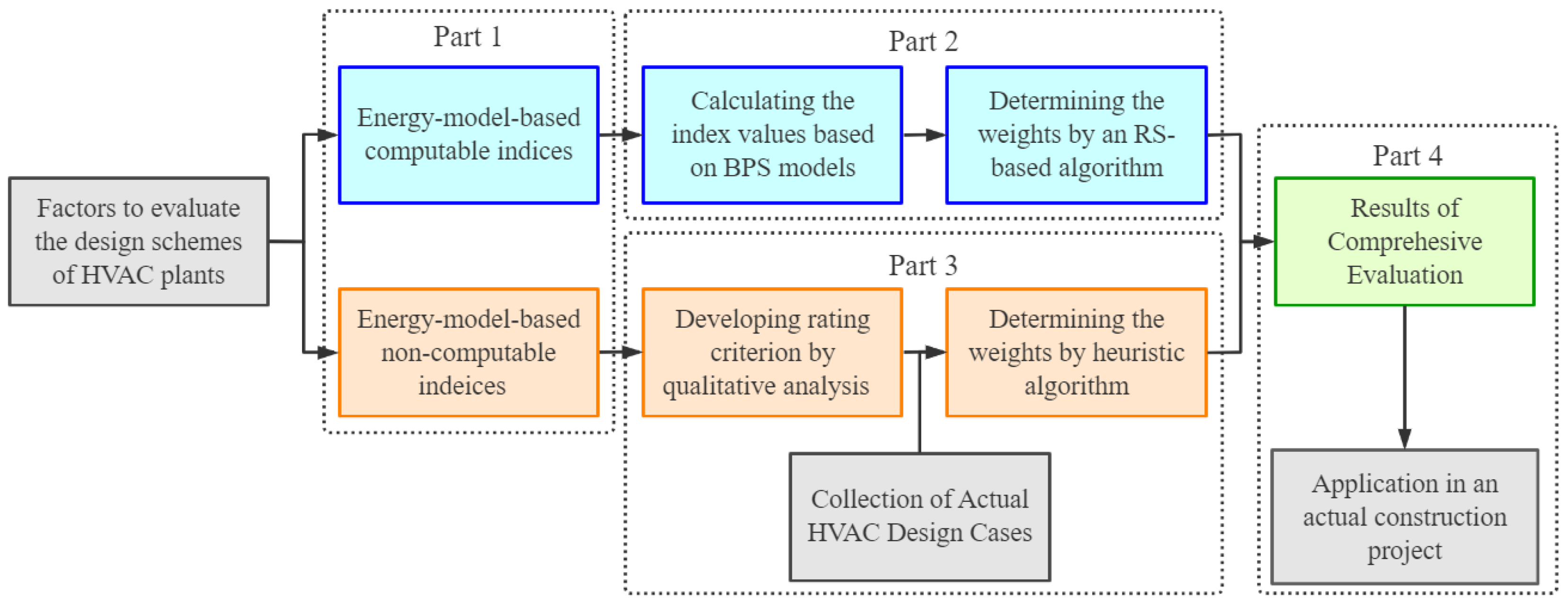However, other aspects such as initial investment costs, difficulty of installation and maintenance that cannot be output by BPS models also have significant effects on the final decision-making process [23]. Since the information about the building and the HVAC equipment is usually insufficient for a detailed analysis during the pre-design stage, decision makers often make judgments based on experts’ previous experience when considering these aspects. To obtain a more accurate evaluation result, this paper covers two parts: for the former category that is denoted as computable index (based on BPS models), a database of BPS models is used as a foundation to compute the values and then determine the weights through an RS-based approach; and for the latter part that is denoted as non-computable index (based on BPS models), a technique based on heuristic optimization is developed to codify experts’ experience into compiled information, which makes the detailed analysis of those non-computable indices feasible.

The main goal of this paper is to establish an integrative evaluation method that contains multiple relevant indices to provide a comprehensive and reasonable assessment for the plant room of centralized HVAC systems in commercial buildings, which is different from the current common method of using only a single index for evaluation. In the new evaluation method, the theory of decision science is applied to a practical issue: comprehensively evaluating the performance of an HVAC plant room, which is a complicated decision-making process that requires a substantial number of working hours. In this process, BPS models and experience information are both utilized to obtain the final results through a new approach developed in this study, thus improving the design quality and reducing the design costs.

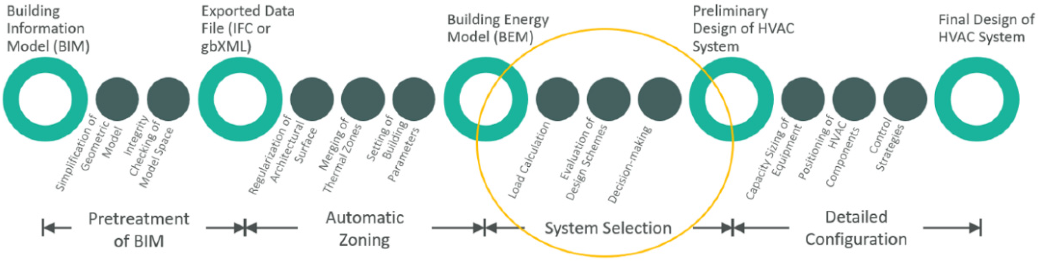
This new method will also be a helpful supporting tool for decision making in HVAC design and construction projects to enhance the quality of the design process and also to reduce the costs of the design work. For example, the method provides a unified standard for discussion between parties before the decision-making process in a construction project for a commercial building (especially when the decision maker of one party is not a professional in building energy system design); and for the “Automatic design of an HVAC system” (as illustrated in Figure 1). The work flow of this new concept can be divided into four tasks: pretreatment of BIM (Building Information Model), automatic zoning, system selection, and detailed configuration. Some researchers in recent years have emphasized the importance of the task of system selection, which means they want to generate the appropriate design scheme of an HVAC system automatically (as highlighted by the yellow circle in Figure 1) [24]. The current project will support this idea by programming the method for a BIM software plug-in such as Revit.

Generally, this paper proposes a novel idea to realize a complicated decision-making process in the design of air-conditioning system plants: selecting the most applicable design schemes of the plants in the building. In the traditional workflow, this process is usually completed manually by professionals. From the perspective of engineering application, it is extremely appreciable for the designers because this evaluation method is actually equivalent to quantifying the fuzzy information (the experience of these designers for the decision making) into a set of compiled rules. Meanwhile, this study also makes an innovative contribution to the research field of the evaluation of HVAC systems: the approach to determine the weight factors— “a hybrid method of RS theory and heuristic algorithm”. Especially in the application of heuristic algorithm, this paper presents a totally new technology to transfer the task of determining the combination of the weights into a global optimization problem, which makes it possible to extract experiment information from the constructed design cases. This provides a good reference for the researchers who are interested in similar topics. They can apply the same idea to realize the integrated evaluation for more components and systems in buildings, so as to improve the design quality and reduce the costs during the whole process of architectural design.

2. Methodology

The specific research methodology of this study is as follows (Figure 2):

• Classification of indices: all indices covered in this paper are classified into two categories: BPS-model-based computable indexes and non-computable indexes according to whether they can be calculated directly from the outputs of BPS models.
• Evaluation based on BPS models: as the computation basis, a pre-simulated model database is briefly introduced to show its data structure and physical properties. Then, the approaches to calculate the normalized values of computable indices from BPS models are presented. Finally, an importance reduction algorithm based on RS theory is applied to determine the weights or to reduce redundancy indices.
• Compilation of experience information: firstly, for the non-computable indices, an empirical rating criterion is designed to give them quantified scores. Then, a collection of actual HVAC design cases is used to reflect experts’ experience of realistic projects—some unquantifiable factors that affect professional engineers when deciding on the best design solution are examined. Finally, to compile the experience information needed to determine the weights of the non-computable indices, this paper proposes a technique to transfer the problem into a scenario of global optimization, which can be solved by a heuristic algorithm (the genetic algorithm is used in this study).
• Application of the new approach in the design stage of a practical building project. The evaluation results given by this method are compared with the actual decisions made by experts in a realistic project. Therefore, the utility of this comprehensive evaluation is verified.

2.1. Classification of Indices

The first step of this methodology is to summarize all the factors that might affect the decision makers in the selection of the design schemes of the HVAC plant room. As discussed above, some indices can be output from BPS models, which are regarded as a computable index, considering that energy modeling is commonly used in the design stage of most building projects. This means that the statistical characteristics of these indices can be analyzed through pre-simulated models during a normal design process. Meanwhile, there are other factors that are not as easily quantified by BPS models but which have a significant impact on the evaluation. This information is the tacit knowledge of experts. In this study, this type of information is regarded as a non-computable index. The methods to determine the weight factors of these two different types of indices could be different; therefore, we combine the total score of the evaluation object to include two parts: the score of computable indices and the score of non-computable indices (Equation (2)).

$$T=\left(1-\alpha \right)·CI+\alpha ·NI$$

(2)

where T refers to the total score of an evaluation object; NI refers to the total score of all non-computable indices; CI refers to the total score of all computable indices; and α refers to the ratio of the value of NI to T.

All indices covered in this study are listed in

Table 1. Classification of all indices in this study.

Category	Index
Computable index (based on BPS models)	Total specific energy consumption for cooling/heating per floor area (equal to standard coal) (TECc/TECh)
	Annual energy cost for cooling/heating in the life cycle per floor area (AECc/AECh)
	Exergy cost per unit of cooling and heating energy (XCEc/XCEh)
Non-computable index (based on BPS models)	Actual perception of the occupants on thermal conditions
	Impact on ambient environment
	Capital cost of plant equipment
	Difficulty of installation and maintenance costs

. It should be noted that the non-computable index in this paper refers to the index whose value cannot be output through the BPS model, but this does not mean that its value can never be calculated. For example, the indoor thermal comfort, the capital cost of plant equipment and the difficulty of installation and maintenance are all classified as non-computable indices, since modelers can hardly compute the exact values of their values just using a BPS model, although these indices can be quantified by some variables such as the Predicted Mean Vote (PMV) and the Life Cycle Cost (LCC).

For the computable index, the following 6 indices are selected for the further analysis: TECc, TECh, AECc, AECh, XCEc, and XCEh. These indices are the variables that can be easily computed by BPS models. Thus, Section 2.2 will first provide a brief introduction to the pre-simulated model database used in this study, and then explain the computation process of the computable indices and their weights in the evaluation. For the non-computable index, Table 1 only lists the description of these indices, while their specific meanings will be detailed in Section 2.3.

2.2. Evaluation Based on BPS Models

2.2.1. Calculation of Computable Indices

As the foundation of this study, a commercial building energy simulation database was established earlier (Zhu, 2019) [25]. A brief introduction to this pre-simulated database based on EnergyPlus models is provided in Appendix A. In this model database, the simulation results contain the energy consumption of the building and HVAC system as well as the sub-system energy consumption and many other variables that can be output hourly for the entire year, which are used to calculate the values of computable indices for the following study.

In this paper, the six computable indices include TECc, TECh, AECc, AECh, XCEc, and XCEh. For TECc, TECh, AECc, and AECh, they can be easily computed according to the energy consumption data, conversion factors of standard coal, and prices of various energy sources. XCEc and XCEh are two indices that represent the conversion efficiency of energy based on the concept of exergy cost, which means an exergy analysis of the complete HVAC system must be carried out before determining the calculation process for these two indices.

Exergy analysis is a mature method to appraise the efficiency of a thermal system. Keenan et al. first proposed the method in the 1950s, and initially its main application was for the analysis of power generation systems [26]. After the 21st century, its application in research into HVAC systems began to emerge. In the periods of 2000–2005 and 2005–2010, the International Energy Agency (IEA) conducted research and produced Annex 37: Low Exergy System for Heating and Cooling of Buildings [27], and Annex 49: Low Exergy Systems for High-performance Buildings and Communities [28]. Taking this as an opportunity, researchers have launched many related works [29,30]. Exergy analysis has been developed into a mature tool for the evaluation of HVAC systems, so we will directly use this method in the following paragraph.

To characterize the grade of energy, physicists use exergy to represent the part of the energy flux that can be transformed into mechanical work in a reversible process. In an exergy analysis, the index of the exergy efficiency is usually used to indicate the energy-using performance of a thermal system. To determine how to compute the index values of energy efficiency based on BPS models, we conducted a brief exergy analysis for the cooling and heating modes of a typical HVAC system in commercial buildings. In this paper, a black box exergy flux model is used to analyze the total exergy gain and loss of the system [31] (shown as Figure 3) because there is no need to focus on the thermo-physical process inside the system. The exergy efficiency of the whole system can be calculated by Equation (3):

$${\eta }_{\mathrm{ex}}=\frac{E{x}_{\mathrm{ef}}}{{\displaystyle \sum }E{x}_{\sup }}=1-\frac{E{x}_{\mathrm{ls}}}{{\displaystyle \sum }E{x}_{\sup }}$$

(3)

where η_ex refers to exergy efficiency; Ex_ef refers to effective exergy; ∑Ex_sup refers to total exergy supply; and Ex_ls refers to exergy loss.

Figure 3 shows that for the whole system, the total supply exergy comes from the energy consumed by the HVAC sub-systems and products (for electric-driven chillers, water pumps, terminal air handling equipment, cooling towers and other components, the exergy is from the municipal power supply; for gas boilers and absorption chillers, the exergy is from gas or steam provided by the energy station). The occurrence of exergy loss in the system is too complex to measure for calculations. Therefore, the total effective exergy that the system produces rather than the exergy loss is usually used to compute the value of efficiency.

The final product of HVAC systems are the air terminal devices that supply cold or hot air to the room space. This part of the cooling or heating energy is finally dissipated into the environment through a variety of heat transfer means. Therefore, the effective exergy of the whole system can be regarded as the exergy flux that the supply air carries. For cooling conditions, the cold air brings cold exergy, and for heating conditions the hot air brings heat exergy (Equation (4)):

$$E{x}_{\mathrm{c}}={\Theta }_0∆S-Q_{\mathrm{c}}; E{x}_{\mathrm{h}}=Q_h-{\Theta }_0∆S; A{n}_{\mathrm{c}\left(\mathrm{h}\right)}={\Theta }_0∆S$$

(4)

where Ex_c refers to cooling exergy; Ex_h refers to heating exergy; Q_c refers to cooling energy; Q_h refers to heating energy; An_c refers to cooling anergy; An_h refers to heating anergy; Θ₀ refers to ambient temperature; and ΔS refers to entropy change.

Nevertheless, these two exergy fluxes are still hard to compute, since the values of entropy brought by the supply air are difficult to obtain from standard BPS models. The users usually do not expect to utilize this energy to generate mechanical work. Thus, it is reasonable to regard the total amount of cooling or heating energy that the system supplies to the indoor space as the output effective energy, and to no longer consider how much energy can be transformed into mechanical work. Similar to the original definition of exergy efficiency, we can define an adapted “exergy efficiency” parameter (Equation (5)):

$${\eta }_{\mathrm{ex}}=\frac{\left|Q_{c\left(h\right)}-{\Theta }_0∆S\right|}{{\displaystyle \sum }E{x}_{\sup }}; {\eta }_{\mathrm{ex}}{}^{\prime }=\frac{Q_{c\left(h\right)}}{{\displaystyle \sum }E{x}_{\sup }}$$

(5)

$$XCEc\left(h\right)=\frac{{\displaystyle \sum }E{x}_{\sup }}{Q_{c\left(h\right)}}=\frac{1}{{\eta }_{\mathrm{ex}}{}^{\prime }}$$

(6)

where η_ex’ refers to adapted “exergy efficiency”.

In this study, the reciprocal of this parameter is used as the evaluation index for a more perfect explanation of the physical meaning of the index. The indices are defined as the exergy cost per unit of the cooling/heating energy (XCEc and XCEh), which indicates the total external exergy supplied to the system to obtain a unit amount of cooling or heating energy as the product (Equation (6)).

For the method developed, we have transferred Equation (4) into a form that only contains the variables available from the pre-simulated model database, as in Equations (7) and (8). The inputs include the annual cooling/heating energy, the total energy consumption of the HVAC system, and the sub-metering energy consumption of the cooling/heating plant (chillers, boilers, and heat pumps), the air distribution system, and the cooling tower and the pumps of the HVAC system:

$$XCEc=\frac{1}{Q_{c,a}}\left[k_s{E}_s+k_e\left(E_{tw}+E_{p,c}+E_{f,h}\right)\right]$$

(7)

$$XCEh=\frac{1}{Q_{h,a}}\left[k_s{E}_s+k_e\left(E_{p,h}+E_{f,h}\right)\right]$$

(8)

where Q_c,a refers to annual cooling energy; Q_h,a refers to annual heating energy; k_s refers to the average exergy cost of the energy source that the chiller or the heat pump consumes; k_e refers to the average exergy cost of electricity; E_s refers to the annual energy consumption of cooling/heating sources; E_tw refers to the annual energy consumption of cooling tower; E_p,c refers to the annual energy consumption of pumps for cooling; E_p,h refers to the annual energy consumption of pumps for heating; E_f,c refers to the annual energy consumption of fans in the terminal device for cooling; and E_f,h refers to the annual energy consumption of fans in the terminal device for heating.

For k_s, it will be denoted as k_g when the energy source is gas and k_e when the energy source is electricity. Here the value of k_g is specified as 1.0, and the value of k_e as 1.8. These are the average values according to the general situation of energy efficiency for power generation. For the absorption chiller, it is assumed that the source to produce steam is a gas boiler with 85% energy efficiency.

For the other four indices that are easier to calculate, the specific equations used in this paper are also provided below (Equations (9) and (10)):

$$TECc\left(h\right)=c{e}_e{E}_e+c{e}_g{E}_g$$

(9)

$$AECc\left(h\right)=\frac{1}{Y}{\displaystyle \sum }_{y=0}^Y\left[\left(p{e}_e{E}_e+p{e}_g{E}_g\right){\left(1+r\right)}^{-y}\right]$$

(10)

where ce_e/ce_g refers to the conversion coefficient of a standard coal plant (0.1229 kgce/kWh for electricity and 1.3300 kgce/m³ for gas); pe_e/pe_g refers to the price of energy sources (1.20 CNY/kWh for electricity and 3.50 CNY/m³ for gas); Y refers to the years of use of an HVAC system (it is specified to be 10 years); and r refers to the annualized rate of return (it is specified to be 5% per year according to the average return on investment).

Since the values of these indices are only used to reflect the applicability and suitability of different design schemes for evaluation, the relative size between these values is important to this study rather than the absolute values. Therefore, although some calculation parameters are determined in reference to the situation in China [32], this methodology will still be valid for application in other regions.

According to Equations (7)–(10), the EnergyPlus models in the database can output all the required inputs for index calculation. In the settings mode of EnergyPlus, modelers can edit the output variable list of each model. For an arbitrary model in the database, all simulation results of the hourly values of the required outputs are added together to obtain the annual value according to the division of the cooling and heating period. Then, all the index values are computed in an automatic process. Finally, we obtained 18,135 groups of index values, which form a “multi-index set”.

2.2.2. RS-Based Knowledge Reduction Algorithm

After the calculation of the values of all six computable indices, the next challenge is to integrate them into a final value of CI in Equation (2). This paper proposes a knowledge reduction approach based on RS theory to do the integration. RS theory is a set of principles based on the set theory. In recent years, many researchers have used it to analyze complex engineering systems with discrete variables and uncertain information [33], and the application of this method to the analysis of an evaluation system has also been quite common [16,17,18,19,20,21]. In general, the mathematical principle of the RS-based approach is to quantify the importance of six computable indices and then to obtain their weights or even to remove some of them if these indices are redundant for the comprehensive evaluation. The “multi-index set” generated in the previous section is used as the data foundation for this algorithm.

The “multi-index set” contains six indices, each of which records 18,135 groups of index values as the objective data for the knowledge reduction algorithm to count the amount of information carried by these data, which can be used to determine the importance of the indices. Since the element in any rough sets must be discrete, all index values should be discretized in advance. In this paper, the discretization is implemented through the normalization of each index. Specifically, this operation includes the following two steps:

• Finding the maximum and the minimum values of each index in the “multi-index set”. The results are shown in

  Table 2. Extreme values of indices.

  Index	XCEc (J/J)	TECc (kgce/m2)	AECc (CNY/yr)
  Maximum	1.529	19.74	156.3
  Minimum	0.6613	0.9631	7.624
  Index	XCEh (J/J)	TECh (kgce/m2)	AECh (CNY/yr)
  Maximum	1.789	21.16	172.2
  Minimum	0.6257	0.6223	5.061

  .
• Normalizing the index values by Equation (11). In this equation, “rounding up” is denoted as a symbol “⌈⌉”. After the normalization, discretization is also carried out. For each index, 18,135 values are divided into 100 intervals according to the normalized results from Equation (11).

$$NV=\lceil 100\times \frac{max-OV}{max-min}\rceil$$

(11)

where OV refers to the original value of the index; max refers to the maximum value of the index within the “multi-index set”; and min refers to the minimum value of the index within the “multi-index set”.

After all index values have been normalized and discretized, the knowledge reduction approach to screen the important elements in an attribute set in RS theory can be applied for the “multi-index set”. The mathematical principle of the approach is described in the literature [15]. This paper will also present a brief introduction to the mathematical principle in Appendix B.

In the application scenario of this study, there are 18,135 groups of indices in total in the “multi-index set”, which corresponds to 18,135 BPS models (585 different buildings and 31 different types of HVAC system). However, since this paper only focuses on the evaluation of the HVAC plant room, the difference between the different types of HVAC terminals should not be analyzed in this study—only the building models whose HVAC terminals are fan coils with a DOAS (Dedicated Outdoor Air System) are considered as the optional design schemes to be evaluated except for a VRV (variable refrigerant volume) air-conditioning system. This means that there are 11 design schemes of the plant room covered in the default settings of the evaluation method. For simplicity, this paper sets a series of codes to refer to these system types (as shown by

Table 3. Codes to refer to 11 types of HVAC system as the optional design schemes.

Number	Code	Type of Cooling/Heating Source	Code	Type of Pumps
1	S1	Centrifugal chiller and boiler	P1	Constant flow
2	S1	Centrifugal chiller and boiler	P2	Variable flow
3	S2	Screw chiller and boiler	P1	Constant flow
4	S2	Screw chiller and boiler	P2	Variable flow
5	S3	Absorption chiller and boiler	P1	Constant flow
6	S3	Absorption chiller and boiler	P2	Variable flow
7	S4	Air source heat pump	P1	Constant flow
8	S4	Air source heat pump	P2	Variable flow
9	S5	Ground source heat pump	P1	Constant flow
10	S5	Ground source heat pump	P2	Variable flow
11	S6	VRV system	-

).

The terminal types of these HVAC systems are all the same, which ensures that the difference between the indices is caused by the performance differences of different plant rooms. Therefore, this multi-index set can be regarded as a summary of 585 different design or construction projects of HVAC systems. For each project, 6 normalized indices are used to evaluate 11 different design schemes of the HVAC plant rooms. Thus, the RS-based knowledge reduction algorithm introduced in Appendix B can be repeated 585 times to obtain the calculation results for all 585 virtual projects, and then the importance of each index can be averaged by the values of sig(a_i) in these projects according to Equation (12) (as illustrated by Figure 4):

$$w_{c,i}=\frac{1}{585}{\displaystyle \sum }_{j=1}^{585}\frac{sig\left({\mathit{a}}_{\mathit{i}}\right)}{{{\displaystyle \sum }}_{i=1}^{6}sig\left({\mathit{a}}_{\mathit{i}}\right)}$$

(12)

$$CI=\frac{w_{c,1}}{w_{c,1}+w_{c,2}}XCEc+\frac{w_{c,2}}{w_{c,1}+w_{c,2}}XCEh$$

(13)

where w_c,1~w_c,6 refer to the weight factors of XCEc, XCEh, TECc, TECh, AECc, and AECh, respectively; and sig(a₁)~sig(a₆) refer to the significances of these six computable indices.

According to both the qualitative and quantitative analysis, it can be found that TECc, TECh, AECc, and AECh are not the core elements in almost all 585 projects, while the significances of these indices are also far less than that of XCEc and XCEh. This means that these three couples of indices are redundant, and a couple of the indices with high significances (XCEc for cooling and XCEh for heating) are adequate for the evaluation. Therefore, the final value of CI should be computed according to Equation (13).

2.3. Compilation of Experience Information

2.3.1. Rating Criterion of Non-Exportable Indices

The score of CI obtained in the previous section is just a part of the final evaluation result. As another part, the value of NI in Equation (2) is the summation of the evaluation result of all non-computable indices. The specific operation of the approach is to compute the NI value, which contains three steps: (1) designing an empirical rating criterion system to give non-computable indices quantified scores; (2) introducing a collection of the actual HVAC design cases as the foundation for the experience information; and (3) using a heuristic algorithm to determine the weight factors of all five non-computable indices based on the experience information introduced in Step 2.

According to the classification in Table 1, the main non-computable factors affecting the decision making in a design project for HVAC plant rooms are summarized in five indices (

Table 4. Settings of the non-computable indices.

Index Name	Area of Influence
IAE	Impact on Ambient Environment
IOC	Indoor Occupants’ Comfort
CCE	Capital Cost of Equipment (for initial investment)
DIMs	Difficulty of Installation and Maintenance (for cooling/heating sources)
DIMp	Difficulty of Installation and Maintenance (for water pumps)

). To avoid ambiguity, the following provides the detailed descriptions of the meanings of these indices. IAE refers to the impact that the plant device has on the ambient environment (e.g., the long-period operation of a ground source heat pump system might change the soil temperature, if a seasonal heat balance cannot be achieved; and the refrigerant leakage of an air source heat pump will aggravate the greenhouse effect, etc.); IOC refers to the indoor occupants’ comfort when the HVAC system is running (e.g., the all-air system or DOAS cannot be used as the room terminal devices when the cooling/heating source is a VRV air-conditioning system, which means that indoor temperature and humidity control with high precision cannot be realized; and the air source heat pumps installed on the top of buildings may cause noise in the neighborhood, etc.); and CCE refers to the capital cost of the HVAC equipment in the plant room for the initial investment; DIM refers to the difficulty of installation and maintenance in both the construction and the operation stages (DIMs for the evaluation of cooling/heating sources and DIMp for the water pumps).

Decision makers usually find it difficult to compute the specific values of such non-computable indices mentioned above in the design stage of a new HVAC system. For application in the evaluation of typical design practice, the specific values of these indices have no direct effect, but the ranking relation between the different scores corresponds to the judgment on the advantages and disadvantages of different design schemes. Thus, this paper provides an empirical rating criterion for the five non-computable indices through the qualitative analysis for the ranking relation between the earlier conducted design schemes for an HVAC plant room (

Table 5. Rating criterion of five non-computable indices.

Index	IAE	IOC	CCE	DIMs	DIMp
100	(S5)	S1, S2, S3, S5	S4 + P1	S6	S6
90			S4 + P2
80			S6	S4
75	S1, S2, S3
70			S2 + P1
60			S2 + P2	S5
50	S4, S6	S4, (S6)	S3 + P1		P1
40			S3 + P1	S1
30			S1 + P1
20			S1 + P2	S2
10			S5 + P1
0	(S5)	(S6)	S5 + P2	S3	P2

).

The codes in Table 3 that refer to system types are also used in Table 5. For example, “S1” refers to all system types with an S1 centrifugal chiller and boiler; while “S1 + P1” refers to systems with an S1 centrifugal chiller and boiler and a P1 constant pump, simultaneously. Moreover, the “(S5)” in the IAE column means that this index takes the value of 100 if the annual heat rejection and absorption can strike a balance and otherwise 0 for the S5 ground source heat pump; and the “(S6)” in the IOC column means that this index takes the value of 50 if natural ventilation is enough to meet the outdoor air demand of the building and otherwise 0 for an S6 VRV air-conditioning system. According to this rating criterion, the score values of all non-computable indices for each one of the 11 design schemes of an HVAC plant room can be obtained in the absence of detailed analysis.

In addition, this paper also defines a conception denoted as Capacity Matching (CM), which refers to whether the peak cooling/heating load and the capacity of plant equipment can match each other (e.g., for a small building with a low cooling/heating load, a centrifugal chiller is evidently not suitable since centrifugal chillers with a small capacity are not common in practice). In the evaluation method, CM is used as a correction factor to adjust the total scores of the evaluation (changing Equation (2) into Equation (14)), which produces the following effects: to reduce the score of those designs that cannot meet the requirement of CM, so that they are excluded from the decision-making results:

$$T=CM·\left[\left(1-\alpha \right)·CI+\alpha ·NI\right]$$

(14)

where CM refers to the correction factor of capacity matching, and it is a Boolean variable.

The calculation of the cooling/heating load is based on BPS models but it is still necessary to evaluate whether it is possible to fulfill the capacity according to the experts’ experience. In this paper, the rules for determining the CM value are formulated, as shown below:

• In order to make mutual standby and switching use possible, the number of chillers in the plant room should usually not be less than 2.
• In general, a centrifugal chiller with a cooling capacity less than 1000 kW is not common in practice; and it is also not common for water-cooled screw chillers or heat pumps with a cooling capacity less than 350 kW in practice.
• According to Rule 2, for an S1 centrifugal chiller and boiler, the value of CM is 1 when the peak cooling load of the building is not less than 2,000 kW, otherwise it is 0; and for S2 screw chiller and boiler and S5 ground source heat pump, the CM value is 1 when the peak cooling load of the building is not less than 700 kW, otherwise it is 0.

2.3.2. Case Collection and Heuristic Algorithm

The determination of the weight factors for non-computable indices depends on the previous experience of professionals. This paper proposes a new approach to collect such information by summarizing the professional knowledge that affects the decision-making process in the design of an HVAC plant room. Besides, before applying the approach to summarize the experience information, a collection of real HVAC design cases should also be established as the foundation of this approach in this study.

In the current research, only the blueprints of these 10 cases have been obtained for further analysis. Thus, this paper utilizes BPS modelling combined with a survey of experts from consulting companies to generate some actual design cases to reflect experiential information. The effect of the additional information is listed as follows:

• According to the data from the blueprints, the BPS models of these 10 original cases can be established. Among them, 6 cases are in Shanghai and 4 cases in Shenzhen (as shown in

  Table 6. Ten real building cases and their basic information.

  No.	Location	Type of Building	Building Area (m2)	Cooling Load (W/m2)	Heating Load (W/m2)	HVAC Plant Room
  1	Shanghai	Office	71,280	101.72	73.60	S1 + P2
  2	Shanghai	Office	40,955	96.50	64.29	S1 + P2
  3	Shanghai	Mall	25,880	130.86	67.04	S1 + P2
  4	Shanghai	Hotel	41,973	84.09	66.02	S1 + P2
  5	Shanghai	Hotel	4010	91.34	77.40	S6
  6	Shanghai	Restaurant	4430	140.21	55.11	S6
  7	Shenzhen	Hospital	23,886	123.93	30.60	S2 + P2
  8	Shenzhen	Institute	6889	92.04	17.20	S4 + P1
  9	Shenzhen	Hotel	17,064	86.38	16.14	S2 + P2
  10	Shenzhen	Supermarket	16,898	117.51	16.08	S2 + P1

  ). In this table, the basic information is listed for each case: the location (city name), the type of building, the total floor area, the number of floors, the specific peak cooling/heating load per unit area, the type of cooling/heating sources, and water pumps used in the plant room (the expressions of system types are the same as in Table 3).
• For 6 cases in Shanghai, the settings of the weather data in the original models of these buildings were transferred from Shanghai into Shenzhen to generate 6 new design scenarios (models), each of which is equivalent to the HVAC design for a reference building modeled with the same parameters as the original case but located in Shenzhen. Similarly, the same approach was also used in the other 4 cases in Shenzhen, except that the location was changed from Shenzhen to Shanghai.
• Considering the correlation between climate conditions and cooling/heating load, three other Chinese cities (Beijing, Xining, and Kunming) were selected to represent their climate regions. In the same manner as the same operation in Step 2, for all 10 original cases, the settings for the weather data in the models were changed to Beijing, Xining, and Kunming, respectively. Finally, the collection contained 50 HVAC design cases (10 original and 40 generated cases).
• For all 40 generated cases, the authors of this paper conducted a survey involving experts from an architectural company, TJAD (Tongji Architectural Design Co. Ltd., Shanghai, China) to determine which optional scheme would be adopted if they were responsible for the HVAC design of the created building models. The judgments made by the experts are regarded as the decision results of these generated cases. In addition, to maintain the consistency of the experts’ judgment, the team responsible for the HVAC design of the application case in Chapter 4 and the respondents of this survey were from the same institute (TJAD).

For the established case collection, each of the 50 cases (real or generated) can be regarded as verification data of the decision-making process. In principle, the task of extracting the experience information is equivalent to searching for a set of evaluation criteria to obtain the best decision results. Mathematically, the result of the search is the weight factors of all non-computable indices. This paper presents a technique to transfer this into a global optimization problem, which means that it can be solved by a heuristic algorithm. Here is a description of this technique:

• The BPS models of the buildings in the 50 design cases have been all established. For each building, the actual type of HVAC system can be regarded as the result of a decision-making process that has occurred in a real design project. Then, the types of the cooling/heating source and the water pumps in these models are changed according to Table 3 to generate the corresponding models for another 10 optional designs as artificial reference cases. After the simulation and computation, the values of all indices for both the finally adopted options and other options not selected are obtained.
• The CI can be calculated from the computable indices and their weight factors obtained in Section 2.2, and the CM correction factor can be also determined based on the load calculation. In this case, the only uncertain variables affecting the final score are the weight factors of the 5 non-computable indices and the ratio α (as shown by Equation (14)). This means that the total evaluation score can be computed when the values of α and w_n,i are given. For each building, there are 11 models with different types of HVAC plant room, and they could be sorted according to the total evaluation score (T). On the basis of this score order, the ranking of the finally adopted option in each case is obtained. In other words, for any given set of weight factors, the summation of the rankings of the finally adopted options for all 50 cases (denoted as SR, and obviously 50 ≤ SR ≤ 550) can be output.
• In this study, it is assumed that the final adopted option of every case should have ranked first or as high as possible in the 11 options. Therefore, for a reasonable evaluation method, the values of SR should be as small as possible when applied to the case collection.
• An application scenario of a global optimization problem can be constructed. The optimization variables are the weight factors of all the non-computable indices, and the range of each variable is 0–1. The objective function is the SR computed according to Step 2, and the objective of the optimization is to make the value of SR as small as possible. To solve a global optimization problem, a heuristic algorithm should be used, and in this study, a genetic algorithm was used. After the optimization algorithm converges, the value of each optimization variable is the weight factor of each non-computable index. This final result constructs an evaluation standard that best reflects the experience information contained in the case collection introduced in this paper.

3. Results

3.1. Supplementary of the Case Collection

Based on the operations introduced in Section 3.1 and 10 real building cases listed in Table 6, this paper produced 40 artificial reference cases as the supplementary of the case collection. The survey results from the experts to determine which optional scheme would be adopted for these 40 generated cases are listed in

Table 7. Survey results of 40 generated artificial reference cases.

Case No.	HVAC Plant Room	Case No.	HVAC Plant Room	Case No.	HVAC Plant Room	Case No.	HVAC Plant Room
SZ-1	S1 + P2	BJ-1	S1 + P2	XN-1	S1 + P2	KM-1	S2 + P2
SZ-2	S1 + P2	BJ-2	S1 + P2	XN-2	S2 + P2	KM-2	S2 + P2
SZ-3	S2 + P2	BJ-3	S1 + P2	XN-3	S2 + P2	KM-3	S2 + P2
SZ-4	S2 + P2	BJ-4	S1 + P2	XN-4	S2 + P2	KM-4	S5 + P2
SZ-5	S6	BJ-5	S6	XN-5	S6	KM-5	S6
SZ-6	S6	BJ-6	S6	XN-6	S6	KM-6	S6
SH-7	S1 + P2	BJ-7	S1 + P2	XN-7	S4 + P2	KM-7	S5 + P1
SH-8	S4 + P1	BJ-8	S4 + P1	XN-8	S4 + P1	KM-8	S4 + P1
SH-9	S2 + P2	BJ-9	S4 + P2	XN-9	S4 + P1	KM-9	S6
SH-10	S2 + P1	BJ-10	S4 + P1	XN-10	S2 + P2	KM-10	S4 + P1

. In this table, the abbreviations of city names are used for simplicity—SH, SZ, BJ, XN, and KM refer to Shanghai, Shenzhen, Beijing, Xining, and Kunming, respectively. The simulation results from the BPS models of these 40 generated cases are illustrated in Figure 5. In this figure, the specific cooling and heating loads per unit building area of each case are shown with black and red columns, respectively, to reflect the thermal performance of these buildings.

As can be seen from the results in

Table 8. Weight factors of 5 non-computable indices.

Non-Computable Index	IAE	IOC	CCE	DIMs	DIMp
Weight factor	wn,1	wn,2	wn,3	wn,4	wn,5
Value	0.3790	0.2994	0.0329	0.2853	0.0034

, the case collection after the supplementary can cover more situations of HVAC design projects. In this new collection, there are several buildings with different patterns of thermal performance: high cooling load and moderate heating load, high cooling load and low heating load, moderate cooling load and high heating load, low cooling load and high heating load, and low cooling load and low heating load. For each thermal pattern, there are also many types of buildings including office, mall, hotel, restaurant, hospital, institute, and supermarket. Thus far, it can be considered that the case collection can reflect the decision-making results of the investigated expert team under various design scenarios common in practical construction projects.

3.2. Performance of the Evaluation Method

A series of results should be obtained by only using the evaluation results of the computable indices, before combining the non-computable indices into the integrated evaluation system as a basis for comparison. The specific rankings of 50 cases are illustrated in Figure 6 in the brown columns. Obviously, for the majority of the cases, the actual decisions and the design plans with the highest scores are not the same according to just the CI (SR = 197). Then, the genetic algorithm introduced in Section 2.3 was programmed and run in MATLAB. The result was examined to display the specific rankings of all 50 cases after the optimization (illustrated in Figure 6 in the green columns).

It is clear that the rankings of the majority of the cases are in the 1st~3rd position according to the complete evaluation method. This indicates that the best design schemes judged by the new evaluation method proposed and the professional experts’ decisions have been basically consistent. If the decision made in every case used to reflect the experience information proves to be reasonable, the new method can be considered rational and convincing.

The following definition can be made here: if the ranking value is 1st in one case, it is defined that the evaluation method makes the “right decision” in this case. Specifically, among all the cases in Shanghai (high cooling load and moderate heating load), there are 8 cases with the “right decision”; in Shenzhen (high cooling load and low heating load) the number is 5; in Beijing (moderate cooling load and high heating load) the number is 7; in Xining (low cooling load and high heating load) the number is 7; and in Kunming (low cooling load and low heating load) the number is 6. In a sense, this phenomenon reveals the following conclusion: In general, the evaluation results of the HVAC plant design scheme by this method can basically comply with the judgment of experts’ experience; however, for specific application scenarios, the evaluation method is very effective in the construction project of the building with large cooling and heating load, and the reliability of the conclusion will slightly decline in the case of a small cooling and heating load. At this time, the evaluation results may still need to be reconfirmed by the expert team.

The best results obtained by the genetic algorithm also conclude the values of all weight factors of non-computable indices (as shown Table 8). When the weight factors take these values, SR can take the minimum value (SR = 79).

In addition, the ratio parameter (α) was also determined during the optimization process. To find the best value for α, multiple results were computed as α takes different values (from 0 to 1). For each value of α, the minimum value of SR was output (illustrated by Figure 7). The curve indicates that the SR is the lowest (SR = 79) when α = 0.7, which means the best effect of the evaluation can be realized under this situation.

4. Application in an Actual Case

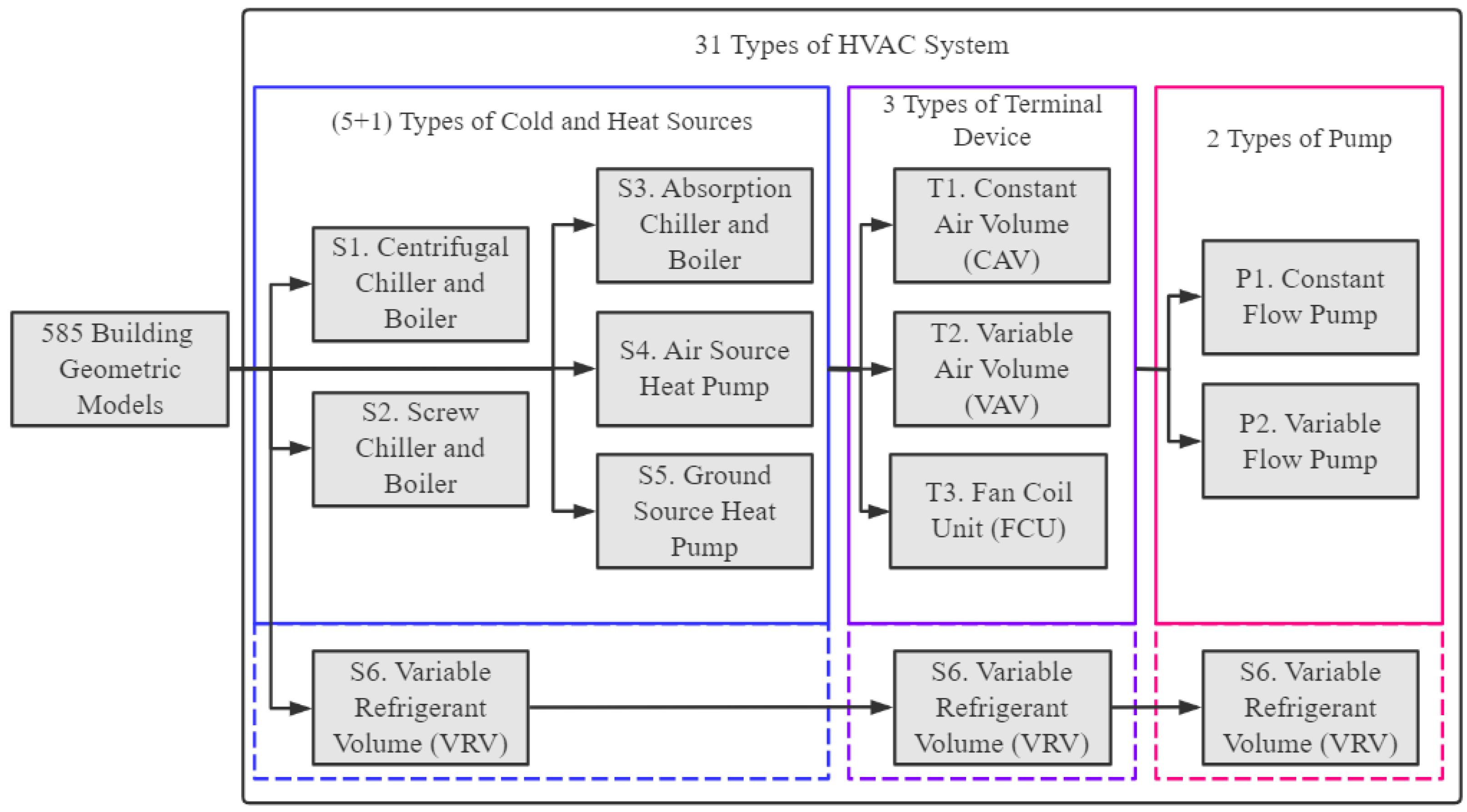
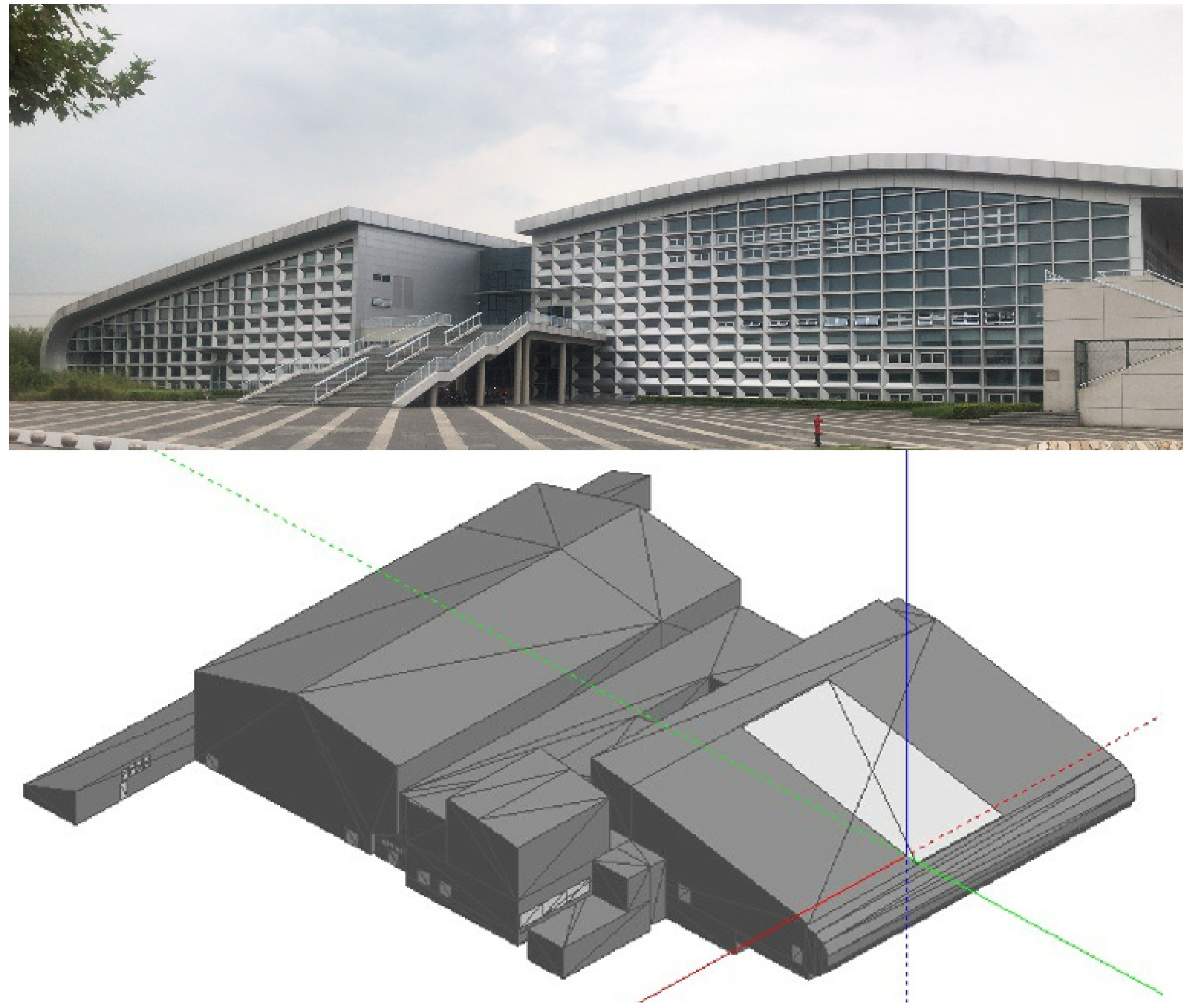
In this section, an actual construction project for a commercial building with a centralized air-conditioning system is taken as an example to show how to apply this method in practice. The example building is a sports center in the suburb of Shanghai, which contains a court, a gym, a swimming pool, as well as shopping and office areas. This case includes two design scenarios from the view of the operating schedule, the building should be divided into two large thermal zones: the core zone that contains the court, gym, swimming pool, and shopping area (the total floor area is 9845 m²) and the office zone (the total floor area is 4890 m²), which means two separate HVAC systems are required for each zone to ensure that these zones with different schedules can operate independently. In this project, the decision makers have decided to adopt different system types for the different zones: an air source heat pump for the core zone and a VRV air-conditioning system for the office zone. To test the rationality of the new evaluation method, the consistency between the evaluation results and the decisions in reality will be checked in this section. We assume that the designers have made a reasonable decision in this actual project, so the finally carried-out design option is regarded as the best design scheme. If the new evaluation method also gives this design scheme a high score, the evaluation results can be considered reasonable.

In the design stage, the designers had already built up the original BPS model of the case building in DesignBuilder (Figure 8). This model can be used as the foundation for further computation analysis.

Table 9. Model parameters of the building case study.

Item	Unit	Value
Location		Shanghai
Building area:
Core zone	m2	9845
Office zone	m2	4890
Envelope:
Heat transfer coefficient of wall (U-value)	W/(m2·K)	0.66
Heat transfer coefficient of roof (U-value)	W/(m2·K)	0.33
Heat transfer coefficient of window (U-value)	W/(m2·K)	2.8
Solar heat gain coefficient (SHGC) of window		0.34
Window to wall ratio		0.37
Indoor temperature set-point (summer/winter):
Swimming pool	℃	28/28
Office	℃	26/20
Other room	℃	26/18
Indoor relative humidity set-point (summer/winter):
Swimming pool		65%/65%
Office		55%/50%
Other room		55%/50%
Outdoor air volume:
Swimming pool (according to the ventilation rate)	ac/h	1
Other room (according to occupant density)	m3/(h·p)	40
Office: (according to the infiltration rate)	ac/h	0.7
Internal heat source:
Lighting power density (core zone/office zone)	W/m2	15/11
Other equipment power density (core zone/office zone)	W/m2	10/15
Occupant density (core zone/office zone)	m2/p	4/8
HVAC plant room:
Cooling and heating source (core zone/office zone)	Air source heat pump/VRV
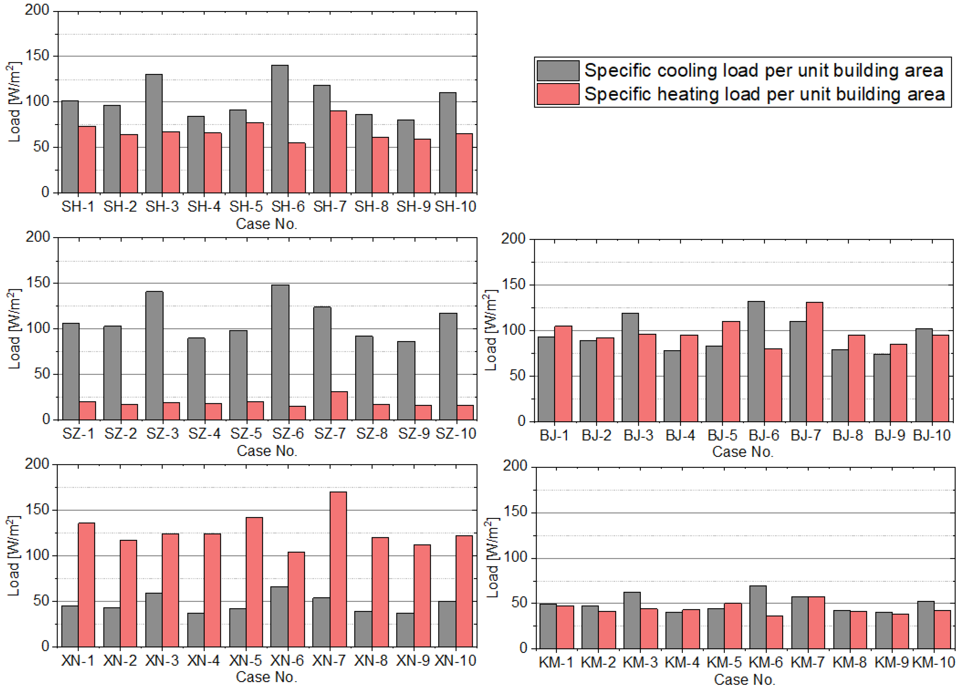
Pumps (core zone/office zone)	Variable flow/VRV

lists the settings of the model parameters, and

Table 10. Simulation results of the cooling and heating loads.

Load	Unit	Value
Core zone:
Peak cooling load per unit area	W/m2	124.6
Peak heating load per unit area	W/m2	83.3
Annual cooling energy per unit area	kWh/m2	69.46
Annual heating energy per unit area	kWh/m2	22.4
Office zone:
Peak cooling load per unit area	W/m2	88.2
Peak heating load per unit area	W/m2	64.7
Annual cooling energy per unit area	kWh/m2	50.35
Annual heating energy per unit area	kWh/m2	16.27

lists the characteristics of the cooling and heating loads of the building as the outputs of the original model. By changing the settings of the type of HVAC plant room in the model, modelers can build up multiple options for models of the buildings with different design schemes. The number of models is equal to how many design schemes are regarded as a final option plan. The outputs of these models are used to compute the values of indices, and then they are weighted and summed up to generate the total rating score for each design scheme. The total score of the option design chosen in the final plan in reality can be also obtained. If the design scheme that is selected by experts in the practical case gains a fairly high total score, it can be considered that the decision made by the new evaluation method is consistent with the experience information.

The total scores of the optional design schemes for both scenarios are listed in

Table 11. Total scores and rankings of optional design schemes for two scenarios.

Core Area			Office Area
Ranking	Design Scheme	Total Score	Ranking	Design Scheme	Total Score
10~11	S1 + P1	0	6~11	S1 + P1	0
10~11	S1 + P2	0	6~11	S1 + P2	0
2	S2 + P1	63.672	6~11	S2 + P1	0
1	S2 + P2	64.096	6~11	S2 + P2	0
6	S3 + P1	57.480	5	S3 + P1	57.007
5	S3 + P2	57.731	4	S3 + P2	57.257
4	S4 + P1	59.867	3	S4 + P1	59.567
3	S4 + P2	60.292	2	S4 + P2	59.992
8	S5 + P1	54.330	6~11	S5 + P1	0
7	S5 + P2	54.581	6~11	S5 + P2	0
9	S6	50.663	1	S6	61.142

. In this table, all the design options are sorted according to their total scores, so the rankings of the final adopted designs (in red) can be easily determined. According to the evaluation results, the design scheme actually adopted in the core area (air source heat pump with variable flow pumps, S4 + P2) ranks 3rd; and the design scheme in the office area (VRV air-conditioning system, S6) ranks 1st. Besides, it can be seen that there are some design schemes whose total scores are zero according to the evaluation results in both of the two indoor scenarios. The zero total score means that CM, the Boolean variable in Equation (14), takes the value of zero in the evaluation of these design schemes. According to the definition, CM is the correction factor to screen out those optional schemes that is inapplicable due to the difficulty to obtain the equipment with appropriate capacity on the market. Therefore, this evaluation method can easily exclude some types of HVAC plants from being the decision-making result. For example, the evaluation results show that the total scores of these two design schemes, S1 + P1 and S1 + P2, are zero in the scenario of the core area. Through the load prediction, the total capacity of the cooling system in this scenario can be calculated: 1226.69 kW. According to the rules introduced in Section 2.3.2, the plant design schemes with the centrifugal chiller cooling source are not appropriate for this building. Finally, this makes the total scores of these schemes zero.

Generally speaking, the design schemes chosen by the professional decision makers of the application case also obtained relatively high scores in the comprehensive evaluation. For the scenario of the office area, the system type of HVAC plant with the highest evaluation score was used in reality. For the scenario of the core area, a screw chiller with a constant or variable flow pump (S2 + P1, S2 + P2) seems to be a better design for the HVAC plant room according to the evaluation result; however, in reality the designers still selected an air source heat pump system as the cooling and heating source. In summary, the results obtained by the evaluation method are basically consistent with the judgment of experts, which can explain the rationality of the comprehensive evaluation method proposed in this paper to some extent.

For the slight mismatch in the evaluation of the design schemes for the core area of the sports center, we infer that the decision makers of the project considered the following factor: there is a constant-temperature swimming pool in the core area of this sports center, and the designers choose the heat pumps to provide hot water for both the HVAC system and the swimming pool. In Shanghai, the energy efficiency of the heat pump to produce domestic heat can be significantly higher than boilers. Thus, for those design schemes of HVAC plants that are not normal (the core area is just an example, in which the designers hope the plants can meet the requirements of air-conditioning and water supply), the evaluation results of this method can be a reference but the final decision-making process still needs to be verified by experts.

5. Conclusions

The present research introduces a new method for making an integrated evaluation of a complex design task (the HVAC plant room in a commercial building). Firstly, we utilized a BPS model database to output indices that reflect the overall energy efficiency of the equipment in HVAC plant rooms, and then applied an RS-based algorithm to remove the redundant indices from them and to determine their weight factors. Secondly, we used a collection of actual HVAC design cases combined with a genetic algorithm to obtain the most reasonable set of weight factors for those indices that cannot be computed directly by BPS models. Thirdly, we analyzed this method in an actual building design project to further verify the rationality of the evaluation result. As the main achievement of this study, a fast-comprehensive evaluation method for decision making in the design of HVAC plant rooms has finally been developed.

However, there are some shortcomings to this study that can be improved in further research. The improvement work could mainly be carried out in following three respects:

• For the “multi-index set”, this was generated by computation according to the outputs from a pre-simulated BPS database. The models in this database were built in EnergyPlus. As is widely known, the computing engine of EnergyPlus can achieve a very high level of precision when calculating the heat transfer in buildings but the precision could be low when calculating the thermal process for HVAC systems. Meanwhile, the input data also plays a significant role that affects the accuracy of the models. Therefore, in this study, it was assumed that the model errors would slightly affect the distribution of the index values. To perfect this defect, a better “multi-index set” could be generated by using the models built in other software (such as TRNSYS and Modelica) with higher precision for calculating the building technical systems, or by collecting the operation data from sufficient numbers of actual design cases of HVAC systems. The new set could be used to obtain new results of the objective evaluation, and the results could then be checked to determine if they change significantly or not.
• For the collection of actual HVAC design cases, this paper hopes to expand the quantity of collected cases as much as possible, while ensuring that the drawing information or operation data is adequate for modeling and to output usable index values. For more convincing results, only the design cases whose actual performance have been proven to be good should be used. This would ensure that the decision made in each project must be reasonable. In this paper, it was assumed that the survey results from the experts of the consulting engineering company would meet this requirement. In the future, with an increase in actual cases collected, the cases will be screened to delete those cases with bad performance, and then a similar method will be used to establish a more convincing design case collection. Since the method introduced in this paper is generic, the results obtained from this study are still meaningful.
• For the theoretical basis of this evaluation method, there are still several flaws that have not been solved in this study. One is that this paper provides an empirical rating criterion for every non-computable index, which means that the evaluation for each single index might not be very accurate and it may also be difficult to expand the number of options for decision making. Since this paper focuses on the establishment of an evaluation system, in other words, the determination of the weight factors, the evaluation method can be considered reasonable if the evaluation results and the decisions made by experts are consistent. When a detailed calculation approach for the non-computable indices in this paper has been developed, or some new HVAC plant room design schemes need to be considered as options, an evaluation system can also be established through the same methodology after updating the rating criteria of indices. Only 11 common types of HVAC plant room systems were considered in this paper. For further analysis, we could expand the evaluation system to cover more design schemes with rare types of system or the combination of multiple types of cooling/heating sources by adopting a similar technical route. Another aspect is a common problem for all decision-making and evaluation methods: Arrow’s Impossibility Theorem. According to this theorem, it is impossible to derive a group preference order from an individual preference order. Therefore, in practical application, the decision makers should use the results of this evaluation method as a reasonable reference rather than as a set of absolute rules for making decisions. Decision makers can see all of the evaluation results for the ranking list of all optional designs, and then they can make a final decision based on the combination of the evaluation result and actual state. Human experience provides insurance against automated decision-making processes.

References

1. Kreider, J.F.; Rabl, A. Heating and Cooling of Buildings: Design for Efficiency, 3rd ed.; McGraw-Hill Inc.: Hightstown, NJ, USA, 2018. [Google Scholar]
2. Bai, X.; Sun, C.; Guo, L.; Wang, H. Tests and analysis on energy consumption of heating ventilation and air-conditioning systems in commercial buildings. J. Chongqing Univ. 2008, 31, 637–641. [Google Scholar]
3. Badea, A.; Baracu, T.; Dinca, C.; Tutica, D.; Grigore, R.; Anastasiu, M. A life-cycle cost analysis of the passive house “POLITEHNICA” from Bucharest. Energy Build. 2014, 80, 542–555. [Google Scholar] [CrossRef]
4. Cui, B.; Gao, D.; Xiao, F.; Wang, S. Model-based optimal design of active cool thermal energy storage for maximal life-cycle cost saving from demand management in commercial buildings. Appl. Energy 2017, 201, 382–396. [Google Scholar] [CrossRef]
5. Du, D.; Pang, Q.; Wu, Y. Modern Comprehensive Evaluation Method and Case Selection, 3rd ed.; Tsinghua University Press: Beijing, China, 2015. [Google Scholar]
6. Saaty, T.L. Decision making with the analytic hierarchy process. Int. J. Serv. Sci. 2008, 1, 83–98. [Google Scholar] [CrossRef] [Green Version]
7. Lee, M.H.; Cheon, D.Y.; Han, S.H. An AHP Analysis on the Habitability Performance toward the Modernized Hanok in Korea. Buildings 2019, 9, 177. [Google Scholar] [CrossRef] [Green Version]
8. Zarghami, E.; Azemati, H.; Fatourehchi, D.; Karamloo, M. Customizing well-known sustainability assessment tools for Iranian residential buildings using Fuzzy Analytic Hierarchy Process. Build. Environ. 2018, 128, 107–128. [Google Scholar] [CrossRef]
9. Hazelligg, G. Systems Engineering: An Approach to Information-Based Design; Prentice Hall Inc.: Upper Saddle River, NJ, USA, 1996. [Google Scholar]
10. Xu, T.; You, J.; Li, H.; Shao, L. Energy Efficiency Evaluation Based on Data Envelopment Analysis: A Literature Review. Energies 2020, 13, 3548. [Google Scholar] [CrossRef]
11. Singh, V.P.; Zhang, J. Information Entropy: Theory and Application; China Water & Power Press: Beijing, China, 2012. [Google Scholar]
12. Shannon, C.E. A mathematical theory of communication. Bell Syst. Tech. J. 1948, 27, 379–423. [Google Scholar] [CrossRef] [Green Version]
13. Sun, W.; Hu, X.; Li, Z.; Liu, C. Identifying the configuration differences of primary schools with different administrative affiliations in China. Buildings 2020, 10, 33. [Google Scholar] [CrossRef] [Green Version]
14. Hamid, T.; Al-Jumeily, D.; Hussain, A.; Mustafina, J. Cyber security risk evaluation research based on entropy weight method. In Proceedings of the 2016 9th International Conference on Developments in eSystems Engineering (DeSE), Liverpool, UK, 31 August–2 September 2016; pp. 98–104. [Google Scholar]
15. Pawlak, Z. Rough Sets: Theoretical Aspects of Reasoning about Data; Kluwer Academic Publishers: Dordrecht, The Netherlands, 1991. [Google Scholar]
16. Sawicki, P.; Zak, J. The application of dominance-based rough sets theory to evaluation of transportation systems. Procedia Soc. Behav. Sci. 2014, 111, 1142–1154. [Google Scholar] [CrossRef] [Green Version]
17. Tiwari, V.; Jain, P.K.; Tandon, P. Product design concept evaluation using rough sets and VIKOR method. Adv. Eng. Inform. 2016, 30, 16–25. [Google Scholar] [CrossRef]
18. Kiluk, S. Dynamic classification system in large-scale supervision of energy efficiency in buildings. Appl. Energy 2014, 132, 1–14. [Google Scholar] [CrossRef]
19. Del Giudice, V.; De Paola, P.; Cantisani, G.B. Rough set theory for real estate appraisals: An application to directional district of Naples. Buildings 2017, 7, 12. [Google Scholar] [CrossRef]
20. Lei, L.; Chen, W.; Xue, Y.; Liu, W. A comprehensive evaluation method for indoor air quality of buildings based on rough sets and a wavelet neural network. Build. Environ. 2019, 162, 1062–1096. [Google Scholar] [CrossRef]
21. Guo, T.; Tang, S.; Sun, J.; Gong, F.; Liu, X.; Qu, Z.; Zhang, W. A coupled thermal-hydraulic-mechanical modeling and evaluation of geothermal extraction in the enhanced geothermal system based on analytic hierarchy process and fuzzy comprehensive evaluation. Appl. Energy 2020, 258, 1138–1181. [Google Scholar] [CrossRef]
22. ASHRAE. ASHRAE Standard 209–2018: Energy Simulation Aided Design for Buildings except Low-Rise Residential Buildings; American Society of Heating, Refrigerating and Air-Conditioning Engineers: Peachtree Corners, GA, USA, 2018. [Google Scholar]
23. ASHRAE. 2020 ASHRAE Handbook-HVAC Systems and Equipment (SI); American Society of Heating, Refrigerating and Air-Conditioning Engineers: Peachtree Corners, GA, USA, 2020. [Google Scholar]
24. Sha, H.; Xu, P.; Yang, Z.; Chen, Y.; Tang, J. Overview of computational intelligence for building energy system design. Renew. Sustain. Energy Rev. 2019, 108, 76–90. [Google Scholar] [CrossRef]
25. Zhu, M. Construction of Minimum Variable Set for Energy Prediction Models of Office Building. Ph.D. Thesis, Tongji University, Shanghai, China, 2019. [Google Scholar]
26. Erlach, B.; Serra, L.; Valero, A. Structural theory as standard for thermo-economics. Energy Convers. Manag. 1999, 40, 1627–1649. [Google Scholar] [CrossRef]
27. IEA ECBCS Annex 37: Low Exergy Systems for Heating and Cooling of Buildings. Available online: http://www.ecbcs.org/annexes/annex37.html. (accessed on 20 January 2021).
28. IEA ECBCS Annex 49: Low Exergy Systems for High-Performance Buildings and Communities. Available online: http://www.annex49.com/materials.html. (accessed on 20 January 2021).
29. Balta, M.T.; Dincer, I.; Hepbasli, A. Performance and sustainability assessment of energy options for building HVAC applications. Energy Build. 2010, 42, 1320–1328. [Google Scholar] [CrossRef]
30. Ahamed, J.U.; Saidur, R.; Masjuki, H.H. A review on exergy analysis of vapor compression refrigeration system. Renew. Sustain. Energy Rev. 2011, 15, 1593–1600. [Google Scholar] [CrossRef]
31. Wang, L. Thermodynamic Analysis of HVAC Systems Based on Exergy Method. Ph.D. Thesis, Hunan University, Changsha, China, 2012. [Google Scholar]
32. Zhou, W.; Zhou, C.; Shi, C.; He, G. Rough Set Theory and Application; Tsinghua University Press: Beijing, China, 2015. [Google Scholar]
33. GB/T 2589–2020. General Rules for Calculation of the Comprehensive Energy Consumption; Energy Fundamentals and Management: Beijing, China, 2020. [Google Scholar]
34. China Academy of Building Research. Design Standard for Energy Efficiency of Public Buildings GB50189–2015; China Architecture & Building Press: Beijing, China, 2015. [Google Scholar]
35. Qian, Y. Concise Design Handbook for Air Conditioning System, 2nd ed.; China Architecture & Building Press: Beijing, China, 2017. [Google Scholar]
36. Polishchuk, Y.V. Monitoring of the information entropy for the description of large technical systems. Mechatronics. Autom. Control 2015, 16, 396–401. [Google Scholar]
Figure 1. The topic of this paper and the “Automatic design of an HVAC system”.
Buildings 11 00522 g001
Figure 2. Description of the methodology of the process.
Buildings 11 00522 g002
Figure 3. Black-box exergy flux model of a typical HVAC system.
Buildings 11 00522 g003
Figure 4. Weight factors of the computable indices.
Buildings 11 00522 g004
Figure 5. Specific rankings of 50 cases before and after the optimization.
Buildings 11 00522 g005
Figure 6. Specific rankings of 50 cases before and after the optimization.
Buildings 11 00522 g006
Figure 7. Minimum values of SR when α changes.
Buildings 11 00522 g007
Figure 8. A sports center and its BPS model in a case study.
Buildings 11 00522 g008