openVFIFE: An Object-Oriented Structure Analysis Platform Based on Vector Form Intrinsic Finite Element Method

Abstract

The vector form intrinsic finite (VFIFE) method is a new and promising structural analysis technique that has many advantages as compared with the conventional finite element method (FEM) in analyzing the complex behaviors of a structure. However, despite the popularization of its application in civil and infrastructure engineering, there is no available unified general analysis framework for it, which limits the applications and developments of VFIFE. This work develops and implements a platform (termed openVFIFE) based on a new proposed object-oriented framework to facilitate the development and application of the vector form intrinsic finite method as well as the efficient and accurate analyses of complex behaviors for civil structures. To validate the platform, a series of numerical examples are conducted. Furthermore, to extend the applications of VFIFE, the nonlinear dynamic and collapse processes of a transmission tower under earthquake load are studied using openVFIFE. The results of these numerical examples simulated by the developed truss or beam elements are consistent with theoretical solutions, previous research or conventional finite element models. The failure modes of the transmission tower under earthquake load simulated by the platform is consistent with those observed in real cases. In addition, the results of nonlinear dynamic analyses of the transmission tower show that the computational efficiency of the proposed platform is 6-10 times higher than that of the conventional finite element method. The results provide sufficient evidence to prove the accuracy and efficiency of the proposed platform in the static, dynamic and elastoplastic analyses of truss and frame structures, especially in the structure analysis characterized by strong geometry nonlinearity. It is noteworthy that in addition to the link and beam elements, further work is undergoing on implementing more elements, such as shell and solid elements. The openVFIFE also allows researchers who are interested in this topic to put their creative ideas into this platform and continuously improve the completeness and applicability of the VFIFE method.

1. Introduction

Conventionally, the finite element method (FEM), finite difference method (FDM) or lumped mass method has been widely employed in analyzing the structure’s behavior in civil or mechanical engineering community. These approaches have been well developed and programmed by mathematically analyzing the structural components based on the continuum mechanics. Recently, some advanced finite element models have also been proposed and applied to more accurately model structure’s behavior, e.g., Roy et al. [1,2,3], Uzzaman et al. [4] and Chen et al. [5]. These results show that the FEM is able to simulate some complex structural behavior, such as the failure modes of self-drilling screw connections for high strength cold-formed steel, the buckling of gapped built-up cold-formed steel channel sections, etc.

However, there are some inherent defects that have no satisfactory solutions. For example, serious distortion of grids could be observed when solving the large deformation problem using the Lagrangian principle in finite element analysis. It also requires considerable computation resources and time to deal with some non-continuum and geometrically nonlinear issues, which is especially difficult in examining the complex behaviors of a large-scale structure system. The vector form intrinsic finite element (VFIFE) method proposed by E.C. Ting [6,7,8] provides an innovative algorithm for analyzing the complex behaviors of a structure, such as large deformations, large overall motions, fragmentation, etc. The structure’s geometrical shape and motion are described utilizing a set of discrete particles in VFIFE. The interactions between particles are simulated by massless elements. In addition, the trajectory of each particle is divided into several segments (called path elements) in which the particle properties remain unchanged. To deal with the structure’s discontinuous behavior, the properties of each particle can be updated at time steps between path elements. In general, as compared with FEM, the VFIFE method has five significant advantages:

(1)

According to the discrete model, the particles and elements can be added or removed freely in the analysis process, and thereby the entire process of the collapse or fragmentation of the structure can be well modeled.

(2)

Inspired by the explicit finite element method, the equation of the motion of each particle is directly formulated by Newton’s second law individually, suggesting that there is no concept of any integrated stiffness matrix. Consequently, this method avoids the issue of ill-conditioned matrices, which can happen in the conventional finite element method.

(3)

Moreover, in contrast to the explicit finite element method, the VFIFE method adopts a procedure of reversed motion rather than the co-rotational technique [9,10] to calculate the pure deformations and internal forces of each element. This treatment avoids the numerical instability of the co-rotational technique in dealing with elements with large deformations.

(4)

To solve the governing equations, an explicit solution procedure, e.g., a second order central difference time integrator, is employed. The computation cost can be therefore greatly reduced as compared with the implicit time integrator, in which the nonlinear governing equations are solved by a complicated iterative process.

(5)

Due to the independence of the elements and particles, the VFIFE is specially suitable for parallel computing [9,11].

Because of these advantages, the VFIFE method has received intensive attention in the past decade by many scholars. At the very beginning, only a few elements were studied, including planar frame elements [7], planar 3-node triangular elements and planar 4-node isoparametric elements [8]. Obviously, they are not sufficient to apply the VFIFE method to analyze the engineering structures. Fortunately, in recent years, many elements have been successfully developed for the VFIFE framework, such as three-dimensional (3D) truss elements [11], 3D frame elements [12], 3D fine beam elements [8,13], 3-node triangular membrane elements [14], 4-node quadrilateral elements [15], 3-node triangular shell elements [16] and 8-node hexahedral solid elements [17]. In addition, the VFIFE method has been extended to the analysis of the complex behaviors of structures. The new algorithms of large deflection analysis [9,15], elastic-plastic analysis [13,18,19], collapse analysis [20,21,22,23], crack propagation analysis [24] and contact analysis [17,25,26] have been successively proposed based on the VFIFE framework.

The continuous development and update of new elements as well as algorithms allow for a wide application of VFIFE in many fields, such as civil engineering [20,21,22,23,24,25,26,27,28,29,30,31,32,33,34,35,36,37], maritime engineering [38,39,40,41,42,43,44,45], mechanical engineering [17] and biomechanics [46]. It is confirmed by these literatures that VFIFE has a great potential for the application to civil and infrastructure engineering. However, the most challenging issue is that above-mentioned studies of VFIFE are implemented by self-programmed codes by utilizing MATLAB or FORTRAN language based on a process-oriented framework, which is no scalability and is unsuitable for developing a large-scale and user-friendly software. Besides, the process-oriented framework can hardly meet the requirements of complicated parallel computing. To the authors’ knowledge, there is no software or platform yet available for VFIFE. This is one of the major obstacles for its development and popularization.

On the other hand, structural analysis software such as ANSYS, ABAQUS, ADINA and OpenSees based on FEM or explicit finite element are very mature. These large-scale software have been developed using object-oriented programming technology (OOP), which is currently believed to be the most promising way for designing a new finite element application [47]. The development of object-oriented engineering software flourished in the 1990s [48,49,50,51,52,53], and some new object-oriented software packages have also been developed to implement new structural analysis algorithms or to extend the capability of existing software [54,55,56,57]. With the support of abstraction, encapsulation, modularity and code reuse in OOP architecture, object-oriented finite element software, particularly those written in C++ language (such as OpenSees), have shown high performance and still provide for the maintainability and extensibility essential in modern software packages.

In this study, a basic computing platform (called openVFIFE) is proposed and implemented to facilitate the development and application of the VFIFE method as well as the efficient and accurate analyses of complex behaviors for civil structures. It is written in C++ language with the standard template library (STL) using OOP architecture. The mathematical implementation of VFIFE is briefly introduced in Section 2. Then, the development of the framework and implementation for the openVFIFE platform is described in Section 3. A series of numerical validations of link as well as beam elements are conducted in Section 4. Finally, the openVFIFE is applied to perform the nonlinear dynamic and seismic-induced collapse analysis of a transmission tower before being compared with the results achieved by a conventional FEM software, i.e., ANSYS. It is noteworthy that the link and beam elements are implemented in openVFIFE; more work is undergoing in developing the shell and solid elements. Besides, the advanced modeling features such as initial geometric imperfection, semi-rigid of structure connections and bolt slip, which will affect the behavior of the structure [58,59], are also under development. It also allows researchers who are interested in this topic to put their creative ideas into this platform and continuously improve the completeness and applicability of the platform.

2. Mathematical Implementation of VFIFE

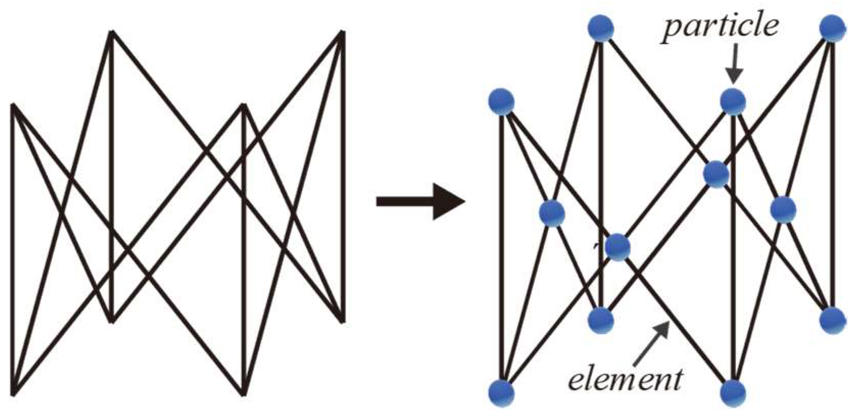
Unlike traditional analytical mechanics, the structure is discretized into a finite number of particles in VFIFE method. These particles are the basic units of the VFIFE. The structure’s geometry and motion are described by the spatial positions and trajectory of the particles, respectively [12]. The structure’s mass, displacement, deformation, boundary conditions, internal force and external force are all determined through each particle. Adjacent particles are connected using a group of standardized elements, such as bar element, beam element, etc. The element is weightless and is only used to calculate the internal force in the particle connected to it. In the time domain, the time trajectory of the particle’s motion is divided into several segments by a series of time points, and the time history of the structure’s motion and deformation is reflected by its displacement, velocity and other state variables at each time point. Assuming that the initial and final time of the analysis is t₀ and t_n, a set of time points $t_0, t_1, t_2,\cdots , t_{i-1},t_i,\cdots , t_n$ is adopted to divide the time history into several independent fragments. The time interval of each segment is small enough such that the physical properties of the particle remain unchanged in each time segment, while the structure’s discontinuous behavior is dealt with at each time point. This discrete scheme of time and space is called point value description. Based on the above discretization method, a 3D truss system can be discretized into a series of particles and elements, as shown in Figure 1. In addition, it is worth noting that VFIFE takes the particle as the basic analysis unit. When considering material nonlinearity, firstly, the strain of the element is calculated according to the deformation analysis results of the element, then the stress of the element is obtained directly according to the stress-strain relationship of the material, and then the internal force of the element is obtained by integration. In this process, it is unnecessary to integrate the global mass and stiffness matrix of the structure system. As a result, the inverse operation of the global stiffness matrix, which is time consuming, is avoided. Thus, it is more efficient than FEM, and more conducive to conducting nonlinear behavior analysis of a structure.

VFIFE directly uses the laws of dynamics as a unified criterion to describe various mechanical behaviors. When describing a structure’s physical behavior, each particle is considered to be in a strict dynamic equilibrium state in the process of motion and deformation. At each time step, the motion of any particle in the structure follows Newton’s second law, and its motion equation is:

$$\begin{array}{c}M\ddot{\mathit{x}}=F_{ext}+F_{int}+F_{damp}\end{array}$$

(1)

where M is the mass matrix, x is the displacement vector, $\ddot{\mathit{x}}$ is the acceleration vector, $F_{ext}$ and $F_{int}$ are the external and internal forces of the particle and $F_{damp}$ is the damping force.

To illustrate the procedures of VFIFE, the space bar assemblies, which have only three translational degrees of freedom (DOFs) on the connected particles, are discussed in this paper [11]. For more information about other types of elements, see [7,8,12,13,14,15,16,17,21]. The mass of a particle connected to a space bar element consists of two parts: the concentrated mass of the particle and the equivalent mass of the space bar element. The mass matrix of the particle can be expressed as:

$$\begin{array}{c}M=\left[\begin{array}{ccc}m& 0& 0\\ 0& m& 0\\ 0& 0& m\end{array}\right], m=m_0+\frac{1}{2}{\displaystyle \sum _{i=1}^n}{m}_i\end{array}$$

(2)

where m is the mass of the particle, m₀ is the concentrated mass and m_i is the mass of the ith bar element.

$F_{ext}$ is the summation of the external forces acting on the particle, which includes the forces directly acting on the particle and the equivalent external forces. The equivalent external forces can be obtained by the principle of virtual work; they have the same form as the results in FEM and are omitted here for brevity.

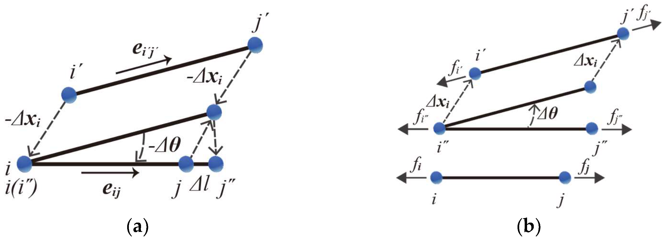
$F_{int}$ is the summation of the internal forces applied by the elements connected to the particle. For one space bar element, the internal element force only depends on its pure deformation. In VFIFE, the rigid body displacement and the pure deformation of an element are distinguished by inverse motion. To illustrate this concept, taking the space bar element shown in Figure 2 as an example, the displacement vector of the end particles i and j at time steps $t_a$ and $t_b=t_a+\mathsf{\Delta }t$ are denoted by (${\mathit{x}}_{\mathit{i}},{\mathit{x}}_{\mathit{j}}$) and (${\mathit{x}}_{\mathit{i}}^{\prime },{\mathit{x}}_{\mathit{j}}^{\prime }$), respectively. Similar to the updated Lagrangian formulations (UL), the configuration of the element at $t_a$ is taken as the reference configuration. From $t_a$ to $t_b$, the relative displacement of particles i and j are $\mathsf{\Delta }{\mathit{x}}_{\mathit{i}}={\mathit{x}}_{\mathit{i}}^{\prime }-{\mathit{x}}_{\mathit{i}}$ and $\mathsf{\Delta }{\mathit{x}}_{\mathit{j}}={\mathit{x}}_{\mathit{j}}^{\prime }-{\mathit{x}}_{\mathit{j}}$; the angle between elements at $t_a$ and $t_b$ can be calculated by:

$$\begin{array}{c}\mathsf{\Delta }\theta =\arccos \left(\frac{{\mathit{e}}_{\mathit{i}\mathit{j}}·{\mathit{e}}_{i^{\prime }{j}^{\prime }}}{\left|{\mathit{e}}_{\mathit{i}\mathit{j}}\right|\left|{\mathit{e}}_{i^{\prime }{j}^{\prime }}\right|}\right)\end{array}$$

(3)

where ${\mathit{e}}_{\mathit{i}\mathit{j}}$ and ${\mathit{e}}_{i^{\prime }{j}^{\prime }}$ are the direction vectors of the elements at $t_a$ and $t_b$, respectively. Let the element at $t_b$ (denoted as $i^{\prime }{j}^{\prime }$) translate $-\mathsf{\Delta }{\mathit{x}}_{\mathit{i}}$ and rotate $-\mathsf{\Delta }\theta$ to $i^{″}{j}^{″}$, as shown in Figure 2a. Then, the pure deformation of element from $t_a$ to $t_b$ can be easily derived:

$$\begin{array}{c}\mathsf{\Delta }l=\left|\mathit{j}{\mathit{j}}^{″}\right|=|(l_{i^{\prime }{j}^{\prime }}-l_{ij}){\mathit{e}}_{\mathit{i}\mathit{j}}|=l_{i^{\prime }{j}^{\prime }}-l_{ij}\end{array}$$

(4)

where $l_{ij}$ and $l_{i^{\prime }{j}^{\prime }}$ are the lengths of the element at $t_a$ and $t_b$, respectively. The axial force in the element at time $t_b$ is:

$$\begin{array}{c}{\mathit{f}}_{{\mathit{t}}_{\mathit{b}}}={\mathit{f}}_{{\mathit{t}}_{\mathit{a}}}+EA\mathsf{\Delta }l/l_{ij}·{\mathit{e}}_{\mathit{i}\mathit{j}}\end{array}$$

(5)

where ${\mathit{f}}_{{\mathit{t}}_{\mathit{a}}}$ is the axial force in the element at time step $t_a$, E is Young’s modulus and A is the cross-sectional area of the element. Note that the internal force calculated by Equation (5) is based on the reference configuration. To obtain the actual internal force at time $t_b$, element $i^{″}{j}^{″}$ should be rotated $\mathsf{\Delta }\theta$ and translated $\mathsf{\Delta }{\mathit{x}}_{\mathit{i}}$ to its original configuration. The magnitude of the internal force will remain unchanged during the rotation and translation except for the direction of the internal force. After the forward motion, the internal forces of the element nodes are:

$$\begin{array}{c}{\mathit{f}}_{{\mathit{i}}^{\prime }}=-f_{t_b}{\mathit{e}}_{{\mathit{i}}^{\prime }{\mathit{j}}^{\prime }}\end{array}$$

(6)

$$\begin{array}{c}{\mathit{f}}_{{\mathit{j}}^{\prime }}=f_{t_b}{\mathit{e}}_{{\mathit{i}}^{\prime }{\mathit{j}}^{\prime }}\end{array}$$

(7)

where ${\mathit{f}}_{{\mathit{i}}^{\prime }}$ and ${\mathit{f}}_{{\mathit{j}}^{\prime }}$ are the internal forces at nodes $i^{\prime }$ and $j^{\prime }$, respectively, and $f_{t_b}$ is the magnitude of the element internal force at time step $t_b$. Axial forces ${\mathit{f}}_{{\mathit{i}}^{\prime }}$ and ${\mathit{f}}_{{\mathit{j}}^{\prime }}$ are applied to the corresponding particles.

Obviously, the VFIFE method is a dynamic analysis method directly based on Newton’s second law. It obtains the dynamic response of a structure by solving the motion Equation of the particles, suggesting that the dynamic analysis is the method’s essential characteristic. However, the energy dissipation of the motion is inevitable due to the effects of damping. The vibration of the real structure will eventually decay to a stable static state. Although different energy dissipation mechanisms result in different trajectories, the structure will converge to a same static stable state as long as the force is unchanged. Therefore, when using VFIFE to solve static problems, the damping force can be assumed arbitrarily. However, when solving dynamic problems, the structure’s real damping parameters should be adopted. To unify the solutions of static and dynamic problems, viscous mass damping is used, and the damping forces are computed from $F_{damp}=\alpha M\dot{\mathit{x}}$, where $\alpha$ is the damping coefficient.

As for the solution of Equation (1), the central difference method is adopted in VFIFE to avoid iteration in the solution procedure. The velocity and acceleration can be approximated as:

$$\begin{array}{c}{\dot{\mathit{x}}}_i=\frac{1}{2\mathsf{\Delta }t}\left({\mathit{x}}_{i+1}-{\mathit{x}}_{i-1}\right)\end{array}$$

(8)

$$\begin{array}{c}{\ddot{\mathit{x}}}_i=\frac{1}{\mathsf{\Delta }{t}^2}\left({\mathit{x}}_{i+1}-2{\mathit{x}}_i+{\mathit{x}}_{i-1}\right)\end{array}$$

(9)

where ${\mathit{x}}_{i-1}$, ${\mathit{x}}_i$ and ${\mathit{x}}_{i+1}$ are the displacements of an arbitrary particle at steps $i-1$, $i$ and $i+1$, respectively, and $\mathsf{\Delta }t$ is the time interval. Substituting Equations (8) and (9) into Equation (1) yields:

$$\begin{array}{c}\{\begin{array}{c}{\mathit{x}}_{\mathit{i}-1}=0.5\mathsf{\Delta }{t}^2{\mathit{M}}^{-1}\left({\mathit{F}}_{\mathit{e}\mathit{x}\mathit{t},\mathit{i}}+{\mathit{F}}_{\mathit{i}\mathit{n}\mathit{t},\mathit{i}}\right)+{\mathit{x}}_{\mathit{i}}-\mathsf{\Delta }t{C}_1{\dot{\mathit{x}}}_{\mathit{i}}, i=0\\ {\mathit{x}}_{\mathit{i}+1}=C_1^{-1}\mathsf{\Delta }{t}^2{\mathit{M}}^{-1}\left({\mathit{F}}_{\mathit{e}\mathit{x}\mathit{t},\mathit{i}}+{\mathit{F}}_{\mathit{i}\mathit{n}\mathit{t},\mathit{i}}\right)+2C_1^{-1}{\mathit{x}}_{\mathit{i}}-C_1^{-1}{C}_2{\mathit{x}}_{\mathit{i}-1}, i\ge 1\end{array}\end{array}$$

(10)

where ${\mathit{F}}_{\mathit{e}\mathit{x}\mathit{t},\mathit{i}}$ and ${\mathit{F}}_{\mathit{i}\mathit{n}\mathit{t},\mathit{i}}$ are the external and internal forces at step i; $C_1=1+0.5\alpha \mathsf{\Delta }t$ and $C_2=1-0.5\alpha \mathsf{\Delta }t$.

3. Framework and Implementation of openVFIFE

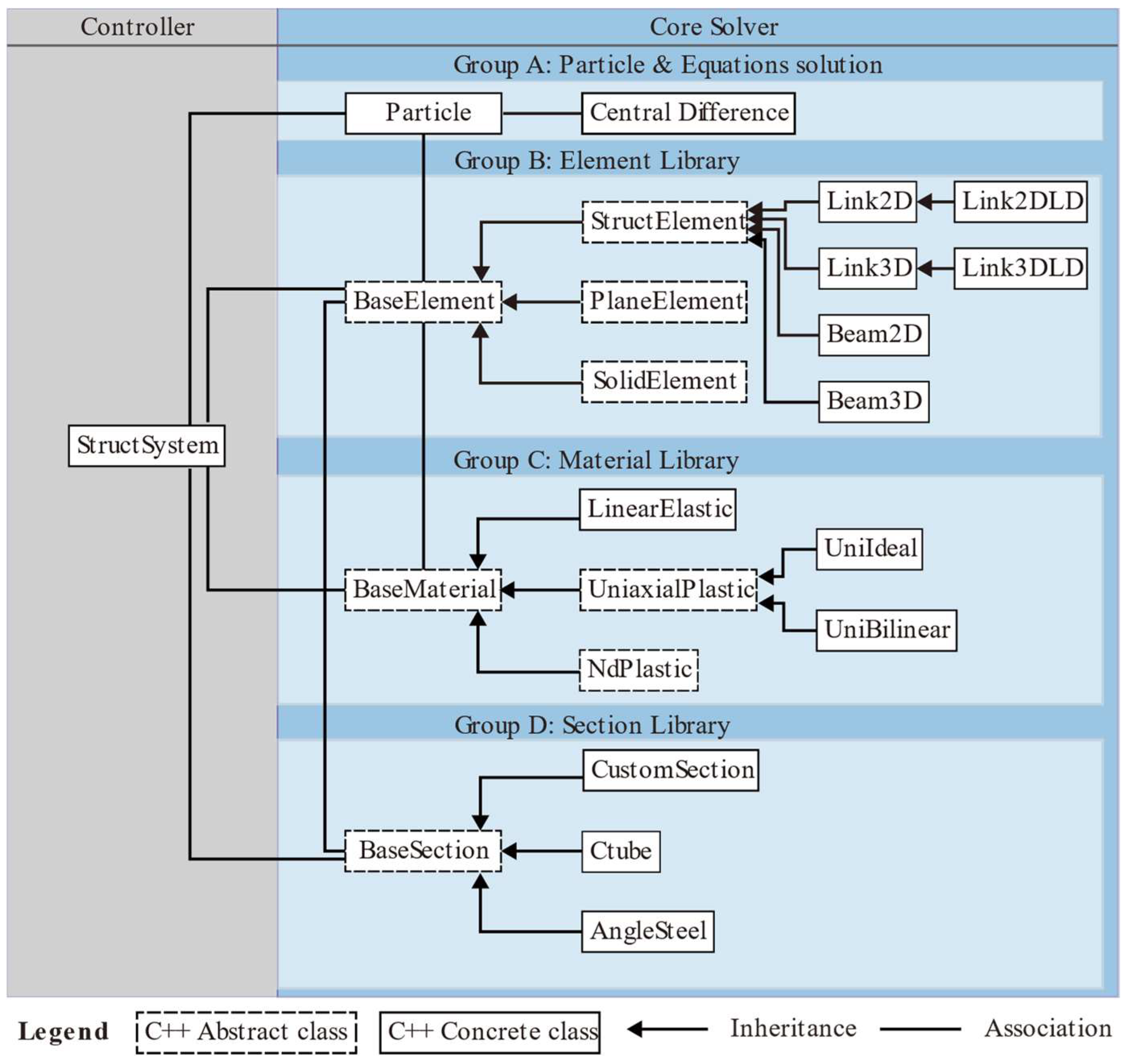
As discussed above, the VFIFE frameworks in the existing literature are based on a process-oriented framework for specific problems. This framework is very easy to implement and has high efficiency. However, it has low code reusability, poor scalability and low maintainability. In this paper, based on the aforementioned theory, an object-oriented framework is proposed, as illustrated in Figure 3. A layered architecture is utilized to design the framework, which is divided into two layers: the controller and the core solver. The controller layer calls the interfaces of the core solver to realize flow control of the analysis procedures. The core solver layer, which consists of particle class (Group A), element library (Group B), material library (Group C) and section library (Group D), is the framework’s foundation. A complex system is divided into several independent modules (also known as modular design) in a layered architecture, which is conducive to simplifying the design and implementation of the program. Based on this layered architecture, the framework proposed here has the following advantages:

• Maintainability. The layered architecture and modular design make the framework easy to be understood, easy to be modified and easy to be tested. Thus, it allows users and developers to modify or improve the framework using their own computer system environment. For instance, if the graphic user interface (GUI) is needed, developers only need to add a presentation layer responsible for GUI above the controller layer without changing the rest of the framework.
• Extensibility. As shown in Figure 3, the class hierarchy is reasonably designed, and the abstract interfaces of the top-level abstract base class are elaborately planned as well, which will be explained in the following sections. Therefore, the analysis code can be modified, extended and recompiled in the framework.
• Developer-friendliness. The framework proposed here assists researchers in using VFIFE for structural analysis. Hence, it must be developer-friendly. Thus, the framework modules are derived from the basic components of VFIFE, which means that each module has a clear physical meaning. For example, the particle class is developed to simulate the behavior of an actual particle in VFIFE. Thus, the whole framework is easy for developers to understand.

The openVFIFE platform based on this framework has the ability to conduct static and dynamic analysis of truss and frame structures. In addition, the elastoplastic analysis and entire-process simulation of the progressive collapse of a structure can also be conducted by openVFIFE. It should be noted that the platform will be supported for a long time and that more new features such as new elements and algorithms will be continuously implemented.

3.1. Particle Class

The particle is the basis of VFIFE. The structure’s motion and deformation are simulated by the particles’ motion. In addition, the deformation analysis of a structural element also needs position information about particles connected to the element. Therefore, the design of a particle class is the foundation of the whole framework. As discussed in Section 2, one particle should have the following information: spatial coordinates, displacement, velocity, acceleration, mass and load. A particle has at most six DOFs, including three translational degrees of freedom (translation in x, y and z directions, denoted by Ux, Uy and Uz, respectively) and three rotational degrees of freedom (rotation around x, y and z axes, denoted by Rotx, Roty and Rotz, respectively). When designing the particle class, the particle’s physical quantities should be reflected in all six DOFs. Unlike FEM, the global stiffness matrix and global mass matrix are not required in VFIFE, so the coding sequence and storage order of particles need not be specially designed. However, in order to ensure the uniqueness of particles in the system, it is necessary to assign a unique identifier to each particle. This identifier not only establishes the topological relationship between the structural element and the particle but is also used for the identification of the particle’s output results. Obviously, the particle contains all the information required to solve the governing equation. In order to reduce the frequency of data exchange in the framework and to ensure the system’s efficiency, the computing of the particle’s governing equation should also be conducted at the particle level.

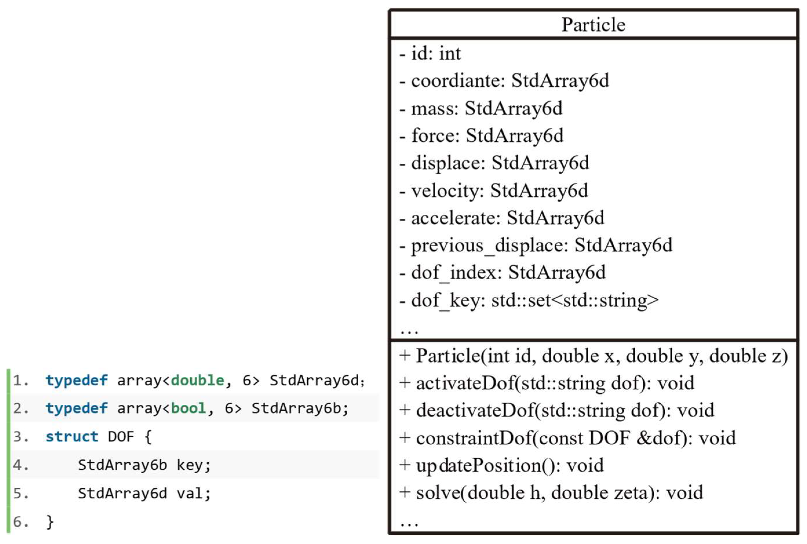
Based on the above conventions, the particle class presented in Figure 4 is established to represent the VFIFE particles. For convenience, efficiency, the security of storage and the usage of data, the following attributes of particle class are stored by an array container in STL: coordinate, force, mass, display, velocity, acceleration and previous displacement. One particle has 6 DOFs, so each position in the array represents information about a fixed DOF, as shown in Figure 5. For different problems, the particle’s DOFs are different. For instance, a particle connected with a space bar element has only three translational DOFs (Ux, Uy, Uz), while a particle connected with a space beam element has all six DOFs. In order to simulate the various combinations of a particle’s DOFs, the dof_key attribute is designed to control them. This attribute is also stored by the array container, and each position corresponds to a fixed DOF and can only be taken as a Boolean value, as shown in Figure 5. When the value in the dof_key[i] (i = 0, 1, …, 5) is correct, the particle has the DOFs corresponding to that position. Correspondingly, three methods, activateDof(), deactivateDof() and constraintDof (), are designed to activate, deactivate and constrain the particle’s DOFs. Furthermore, the particle class includes the solve() method for solving the governing equations. The governing equation is solved by the central difference method, as shown in Equation (10). Once the governing equations are solved, the particle’s spatial position needs to be updated in time, so the updatePostion() method is designed to achieve this function.

3.2. Material Class and Its Derivations

There are many types of materials involved in practical engineering, such as concrete, steel, wood and so on. In the civil engineering field, the mechanical properties of materials are mainly considered, including density, Young’s modulus, shear modulus, Poisson’s ratio and so on. Obviously, it is unreasonable and difficult to integrate material properties into structural elements. Using a material class to simulate materials in practical engineering can take into account the system’s feasibility and extensibility. Depending on the problem, sometimes only linear elastic materials need to be considered, and sometimes nonlinear materials need to be considered. 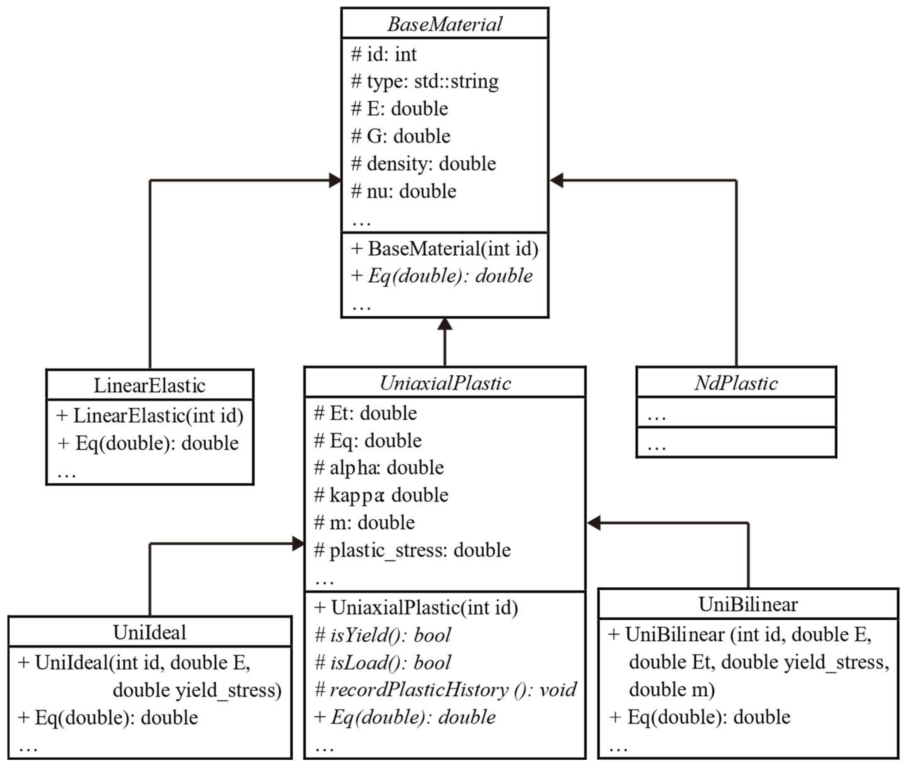Thus, the BaseMaterial class, which serves as an abstract class, is used to specify the necessary mechanical properties of the materials and the interfaces to be called by structural elements. Furthermore, materials with different mechanical properties can be developed according to users’ requirements. The material library shown in Figure 6 is established to simulate elastic and plastic materials.

The abstract base class BaseMaterial is formed by abstracting the commonness of all materials and includes the following main attributes: material number id, material type type, elastic modulus E, shear modulus G and Poisson’s ratio nu. The BaseMaterial class also provides a virtual method Eq() to return the material’s equivalent tangent modulus. The LinearElastic class inherits from BaseMaterial and is used to simulate all linear elastic materials. Two abstract classes, UniaxialPlastic and NdPlastic, are also derived from BaseMaterial and are used to represent plastic materials under uniaxial stress-strain status and plastic materials under complex stress-strain status, respectively. The material properties of plastic materials are related to the loading state and plastic strain/stress history. Therefore, the isYield() and isLoad() methods are designed to determine whether the material yields and whether it is loaded or unloaded after yielding, respectively, as shown in the UniaixalPlastic class diagram in Figure 6. Furthermore, the material’s subsequent yield strength needs to be updated according to its hardening criterion after yielding. Therefore, the method of updateYiledFunc() is designed to simulate the material’s hardening. The method involves four attributes: back stress alpha, hardening parameter kappa, mixed hardening paramePleaster m and plastic stress history plastic_stress.

Table 1. Pseudo-code of the Eq() function for plastic material.

Given a strain increment delta_strain 1. delta_strain_ ← delta_strain // Record the strain increment, 2. Eq_ ← E // initiate equivalent modulus 3. if (isYield()) // Determine whether the material yield according to the yield criteria 4.    then (recordPlasticHistory()) // record the plastic stress and strain history 5.    if (isLoad()) // Determine the load status, load or unload 6.        then (update back stress alpha and growth function kappa, Eq_ ← Et) 7.        else (Eq_ ← E) 8.    else (Eq_ ← E) 9. total_strain ← total_strain + delta_strain 10. total_stress ← total_stress + Eq_ * delta_strain 11. return Eq_

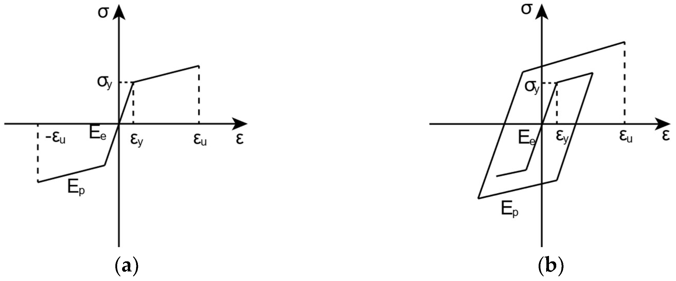
shows the pseudo-code of the Eq() function for plastic material. Depending on the UniaxialPlastic class, two kinds of commonly used plastic material models, ideal elastoplastic model (UniIdeal class) and bilinear elastoplastic model (UniBilinear class), are realized in this paper.

It is obvious that the inheritance mechanism in OOP increases the reusability of codes and is very convenient for programming. The base class BaseMaterial provides a common interface through virtual methods, and the dynamic polymorphism for computing an equivalent tangent modulus by a common instruction is achieved. This mechanism makes it possible to develop a universal solver for VFIFE and also to expand new features for users.

3.3. Section Class and Its Derivations

In truss structure analysis, the element’s stiffness matrix depends on its cross-section characteristics. As in the material library, the section should not be integrated into the element class. It is necessary to design an abstract base class to specify the section characteristics (including area, static moment, moment of inertia, etc.) and the interfaces for calculating them. In the engineering practice, there are various structure members with different sections, so it is unrealistic to establish a derived class for each section. Therefore, it is necessary to design a user-defined section class to simulate the situation where the section properties are given directly. In this way, the section characteristic parameters of an irregular section calculated by other software can be directly used.

Figure 7 shows a UML diagram of the section library. The abstract base class BaseSection has the following properties: section number id, area A, moments of inertia Iyy and Izz and polar moment of inertia Iyz. Correspondingly, the BaseSection class also provides virtual methods calcArea(), calcIyy(), calcIzz() and calcIyz(). In fact, besides the above properties, the section should also have other attributes, such as static moment and shear center, which are not given in this paper due to limited space. The CustomSection, Ctube and AngleSteel classes are inherited from BaseSection and are used to simulate sections with arbitrary parameters, circular tube sections and angle sections, respectively. As stated above, there are many cross-sections of beam and column members in engineering. This paper only provides concrete realization of a few common ones. However, with object-oriented programming, users can easily develop custom section types based on the abstract base class BaseSection.

3.4. Element Class and Its Derivations

In VFIFE, a structural element is used to reflect the internal force response of the structural system under external load, and the internal force in the element is also a part of the external force acting on the particles. When analyzing the internal force in a structural element, it is necessary to first obtain the motion information about the particle connected to it. Deformation analysis according to the particle’s displacement is then carried out to obtain the element’s rigid body motion and pure deformation. Once the pure deformation is obtained, the internal element force can be computed by taking the material and section properties into consideration. Finally, the internal element force is applied to the particles connected to the element as the external force on the particles. The complete procedures are listed in

Table 2. Procedures for element force calculation.

Step 1. Obtain the particle position of the current and previous time step Step 2. Calculate the direction vector of the element Step 3. Calculate pure deformation of the element Step 4. Calculate the increment of strain Step 5. If the element is broken, abort computing and reassign attributes of particles Step 6. Else Step 7. Calculate internal element force Step 8. Endif Step 9. Assign internal force to connecting particles

. It is natural to associate element object with particle object, material object and section object in the framework’s design.

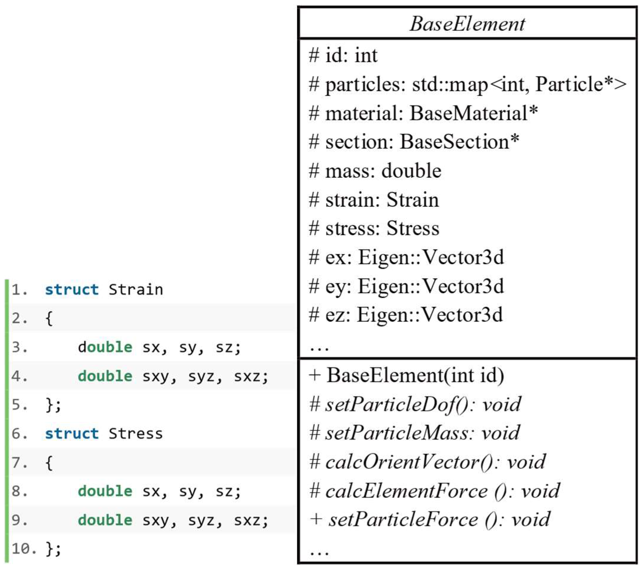
On the other hand, according to the type and scale of the problem, a structural system can be discretized into truss elements (bar and/or beam elements), plane elements, shell elements, solid elements, etc. Obviously, there are many differences among these elements in both geometric modeling and mechanical analysis: (1) a bar element usually contains only two nodes, a plane triangular element can contain three or six nodes, and a shell element and a solid element need at least eight nodes; (2) a truss element must specify element cross-section information, while other elements do not; (3) the material properties that can be considered for each element are different; for example, a bar element cannot reasonably reflect the characteristics of anisotropic materials, while a solid element can fully consider all the mechanical characteristics of anisotropic materials; (4) the rules for establishing the local coordinate systems of elements are not the same; for example, a beam element needs to predetermine its principal axis direction; (5) the stress-strain state of each element is different. In object-oriented programming, the commonness of the above elements is abstracted to form a base element class BaseElement. Besides the basic properties of elements such as particle, material and section, this base class also specifies the methods that elements must have, such as calculating element mass and internal force, as shown in Figure 8.

The abstract base class BaseElement has the following main attributes: element number id, particle objects container particles, material object material, section object section, element mass mass, stress stress, strain strain and direction vector of element local coordinate system ex, ey, ez. The BaseElement class also provides virtual methods setParticleMass(), setParticleMass() and setParticleForce(), which are used to set the DOFs, mass and internal forces in the particles connected to the element, respectively. The virtual method calcOrientVector() is designed to update the element’s local coordinate system. On this basis, the virtual method calcElementForce() is designed to calculate the internal element force.

Furthermore, StructElement, PlaneElement and SolidElement are inherited from the BaseElement class and are used to specify the basic characteristics of truss element, plane element and solid element, respectively. Thus, they also serve as abstract classes. One specific element class can be derived from the above three abstract classes according to its own characteristics. The inheritance relationship of the element class implemented in this paper is shown in Figure 3 Group B.

Link2D, Link3D, Beam2D and Beam3D classes are derived from StructElement class. Link2D element is a 2D bar element that can simulate truss, connecting rod and spring. Each particle of Link2D element has 2 DOFs (Ux and Uy). Link3D is a 3D bar element with similar performance to Link2D, but each of its particles has 3 DOFs (Ux, Uy and Uz). Link2DLD and Link3DLD elements are developed based on Link2D and Link3D elements, respectively, and can consider both geometric nonlinearity and material nonlinearity. Beam2D element is a 2D frame element that can bear axial tension, compression and bending. Each particle of Beam2D element has 3 DOFs (Ux, Uy and Rotz). Beam3D element is a 3D frame element that can bear axial tension, compression and bending. Each particle of Beam3D element has 6 DOFs (Ux, Uy, Uz, Rotx, Roty and Rotz). Both Beam2D and Beam3D elements can consider geometric nonlinearity, but they cannot accurately consider material nonlinearity.

3.5. StructSystem Class

The structural system can be modeled and analyzed utilizing the particle class, material library, section library and element library. However, it has not been unified, and the function of organizing and outputting the results has not been implemented. In order to solve these problems, StructSystem class is designed to manage the particle objects, material objects, section objects and element objects involved in the analysis procedures, as shown in Figure 9. This class is responsible for the creation and destruction of the objects of classes of the core solver, as well as the addition, deletion, checking and modification of each object. At the same time, the StructSystem class is responsible for the output of model information (including particle coordinates, element information and constraint information) and calculation results (including particle motion information and element internal force). The StructSystem class is also the middle layer for users to interact with the core solver of VFIFE. The specific solving process is open to users after being encapsulated by the StructSystem class. This design can not only reduce the cost of users but also increase the security of the whole system.

The StructSystem class has the following properties: number id, working directory workdir, job name jobname, container for Particle objects particles, container for BaseSection objects sections, container for BaseMaterial objects materials, container for BaseElement objects elements and constraint information constraints. The above containers are mainly used to store and manage all kinds of objects in the whole system. In order to facilitate interaction between the user and the kernel, the StructSystem class provides the following methods: setExtetnalForce(), setInternalForce(), autoTimeStep(), solve(), saveResult() and relaseContainers(). Among them, the setExtetnalForce() method is used to apply external load; the setInternalForce() method is used to calculate the internal forces in the elements and apply them to the particle; the autoTimeStep() method is used to achieve automatic time step size; the solve() method calls the particle solver program to solve the governing equation; the saveResult() method is used to save the calculation results; and the relaseContainers() is used to release the contents in the StructSystem class to avoid memory leak.

4. Numerical Validation

As mentioned before, six types of elements are implemented in openVFIFE currently, including Link2D, Link3D, Link2DLD, Link3DLD, Beam2D and Beam3D. Link2DLD and Link3DLD inherit from Link2D and Link3D, respectively. The accuracy and reliability ofLink2DLD, Link3DLD, Beam2D and Beam3D are validated in this section. In addition, the performance of openVFIFE in large deformation analysis, elastic-plastic analysis and dynamic nonlinear analysis is also examined. For example, applications presented in this section demonstrate the aforementioned multiple capabilities of the platform, including the elastoplastic analysis of a planar truss (example 1), stability analysis of a 24-member shallow dome (example 2), large deformation analysis of a planar cantilever beam (example 3) and dynamic analysis of a space curved beam (example 4).

4.1. Example 1: Link2DLD Element

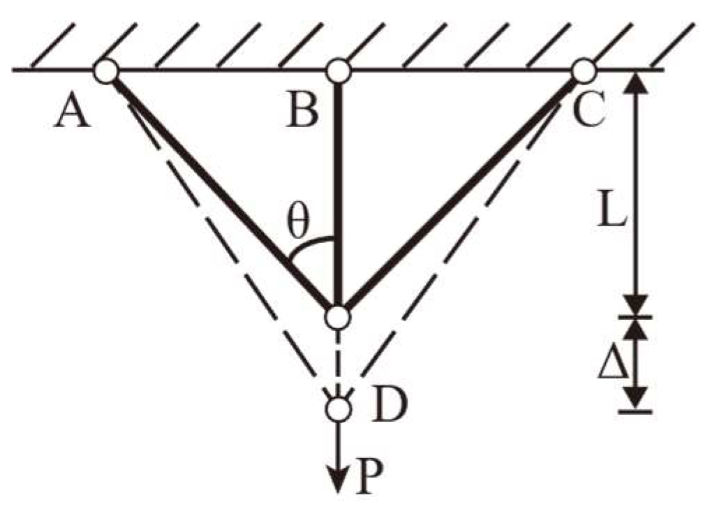
In example 1, a planar three-bar truss subjected to a load P in the y direction is analyzed, as shown in Figure 10. The cross-sectional area (A) of bars is 1 m²; the length (L) of BD bar is 1 m; and $\angle ADB=\angle CDB=\theta =45°$. Two different plastic material models are considered: an ideal elastic-plastic model and an elastic linear hardening model, as shown in Figure 10. The density ($\rho$) of the bars is 7850 kg/m³; Young’s modulus E is 206 Gpa in the elastic state; the tangent modulus E_t is 20.6 Gpa in the plastic state; and the yield stress ${\sigma }_y$ is 235 Mpa.

If the ideal elastic-plastic model is adopted, the displacement of node D can be expressed as:

$$\begin{array}{c}P=\{\begin{array}{c}EA\left(1+{\cos }^3\theta \right)\mathsf{\Delta }/L,P\le P_e\\ {\sigma }_{y}A+2EA{\cos }^3\theta \mathsf{\Delta }/L,P_e<P\le P_y\\ P_y,P_y<P\end{array}\end{array}$$

(11)

where $P_e={\sigma }_{y}A\left(1+2{\cos }^3\theta \right)$, $P_y={\sigma }_{y}A\left(1+2\cos \theta \right)$, and $P_y/P_e\cong 1.41$.

If the elastic linear hardening model is adopted, the displacement of node D can be expressed as:

$$\begin{array}{c}P=\{\begin{array}{c}EA\left(1+{\cos }^3\theta \right)\mathsf{\Delta }/L,P\le P_e\\ {\sigma }_{y}A+E_{t}A\left(\mathsf{\Delta }/L-{\sigma }_y/E\right)+2EA{\cos }^3\theta \mathsf{\Delta }/L,P_e<P\le P_y\\ {\sigma }_{y}A+E_{t}A\left(\mathsf{\Delta }/L-{\sigma }_y/E\right)+2{\sigma }_{y}A\cos \theta +2E_{t}A\cos \theta \left({\cos }^2\theta \mathsf{\Delta }/L-{\sigma }_y/E\right),P_y<P\end{array}\end{array}$$

(12)

where $P_e={\sigma }_{y}A\left(1+2{\cos }^3\theta \right)$, $P_y={\sigma }_{y}A\left(1+2\cos \theta +E_{t}ta{n}^2\theta /E\right)$, and $P_y/P_e\cong 1.47$.

A numerical analysis of the truss is conducted using the proposed framework. The truss is simulated using three Link2DLD elements, which consider material nonlinearity and geometric nonlinearity simultaneously. The time increment $\mathsf{\Delta }t$ is taken as 10⁻⁵ s to ensure the stability of central difference, and the total analysis time t is 100 s. The load P is applied slowly with $\mathsf{\Delta }P=P\mathsf{\Delta }t/t$. 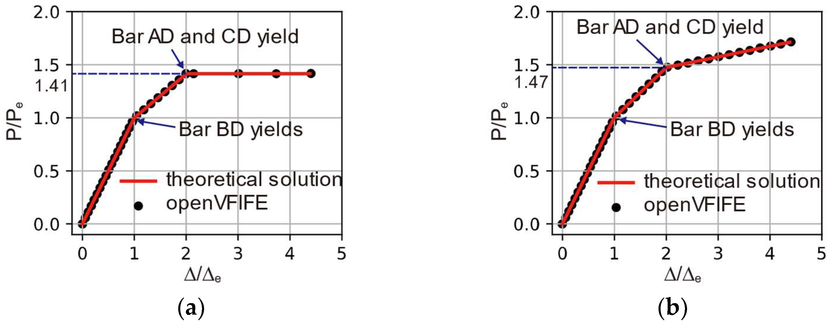The damping coefficient $\alpha$ is taken as 1.0. The dimensionless results of the numerical analysis and the theoretical solution are presented in Figure 11.

As shown in Figure 11, in the planar 3-bar system, BD bar always yields first, and then AD bar and CD bar yield together. For the ideal elastic-plastic model, the truss’s bearing capacity remains unchanged after all three bars have yielded. However, in the numerical analysis, the load is continuously increasing, which leads to a slightly larger numerical result at this stage. For the elastic linear hardening model, the numerical result is consistent with the theoretical result, even when all three bars have yielded. All in all, the openVFIFE results are in good agreement with the theoretical solution for both material models, which proves the feasibility and correctness of the Link2DLD element and openVFIFE. This example also shows that the VFIFE method is suitable for the elastoplastic analysis of a structure.

4.2. Example 2: Link3DLD Element

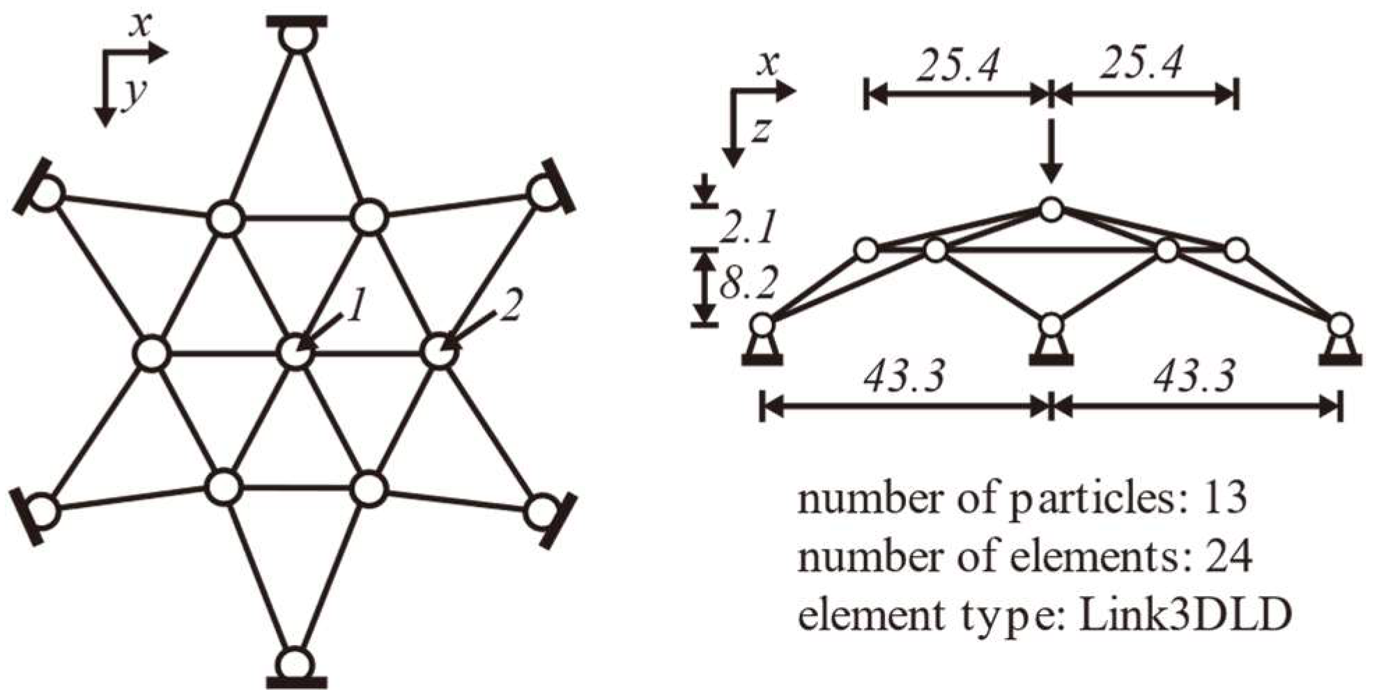
To illustrate the capability of VFIFE in geometric nonlinear analysis, and to test the Link3DLD element, a 24-member shallow dome (as shown in Figure 12) is analyzed by openVFIFE. The topological relationship between elements and particles as well as the size information are depicted in Figure 12. The density of the bars is 20 lb/in³; Young’s modulus E is 10⁶ ksi; and the cross-sectional area (A) of the bars is 0.1 in². A concentrated force P is imposed on node 1 in the z direction, as shown in Figure 12.

The dome is simulated by 13 particles located in the joints and 24 Link3DLD elements. To capture the structure’s buckling process, two loading schemes are adopted here: the displacement-controlled method (DCM) and the load-controlled method (LCM). The computing parameters of openVFIFE are listed in

Table 3. Computing parameters of openVFIFE.

Parameter	DCM	LCM
$\mathrm{time}\mathrm{step}\mathrm{size}\mathsf{\Delta }t$	$1\times {10}^{-3}$ s	$1\times {10}^{-3}$ s
$\mathrm{damping}$	1.0	1.0
$\mathrm{simulating}$	100 s	1000 s
$\mathrm{increment}\mathrm{of}\mathrm{displacement}/\mathrm{load}\mathsf{\Delta }d/\mathsf{\Delta }f$	$6\times {10}^{-5} \mathrm{in}$	$0.5\mathrm{lb}$

. The buckling analysis is also conducted using FEM for comparison purpose. The arc-length method is adopted to capture the complete buckling process, which can provide a benchmark of DCM in openVFIFE. The LCM in FEM is also conducted using same computing parameters as openVFIFE.

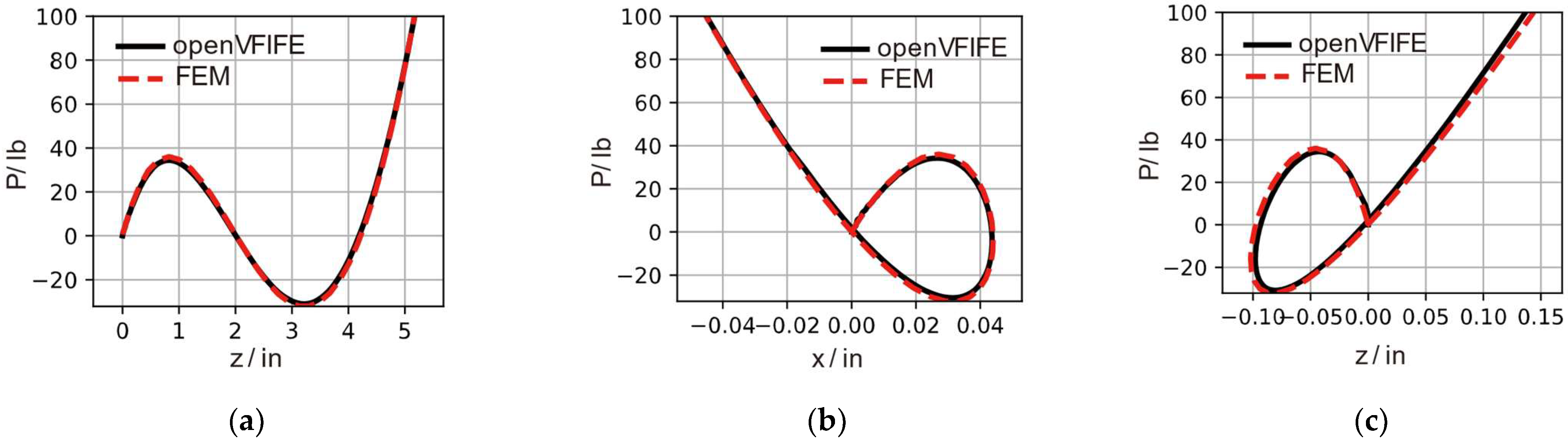
Figure 13 and Figure 14 show load-deflection curves using DCM and LCM, respectively. As can be seen in Figure 13, the load-deflection curves of node 1 obtained by openVFIFE and FEM are quite close, while there is a slight discrepancy for node 2, especially in the z direction. The bearing capacity of the dome increases with the increase of the displacement of node 1 at the small deformation stage. When the dome is instable, the bearing capacity continues to decline. Until the dome stabilizes again, the bearing capacity of the structure can be improved. As shown in Figure 14, the complete instability path can be obtained using DCM. The LCM fails to reproduce the descending portion of the load-deflection curve. Instead, the load remains unchanged after buckling, then increases in the post-buckling position. When the structure is about to buckle, the results calculated by openVFIFE are more consistent with the results using DCM, while the results of FEM are slightly larger. It is obvious that the results of openVFIFE are quite close to FEM, indicating that openVFIFE is suitable for the buckling analysis of a structure.

4.3. Example 3: Beam2D Element

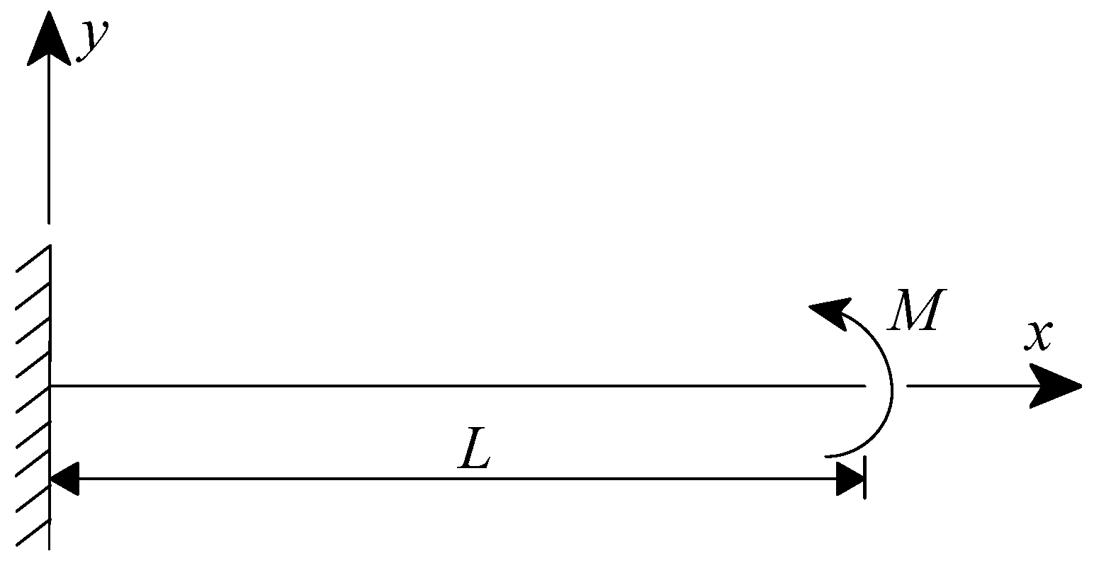
The large deformation analysis of a planar cantilever beam subjected to a bending moment at its free end is shown in Figure 15. Young’s modulus $E$ is $1000\mathrm{pa}$, density $\rho$ is $1\mathrm{kg}/{\mathrm{m}}^3$, beam length ($L$) is $1\mathrm{m}$, cross-section area ($A$) is $1{\mathrm{m}}^2$ and moment of inertia ($I)$ of the cross-section is $0.01{\mathrm{m}}^4$. The beam’s deformation is related to the bending moment acting on the free end, as expressed by:

$$\begin{array}{c}\varphi =\frac{ML}{EI}\end{array}$$

(13)

where $\varphi$ is the curvature.

The cantilever beam is discretized into 21 particles and 20 Beam2D elements. The time step $\mathsf{\Delta }t$ is taken as ${10}^{-5}\mathrm{s}$ to meet the stability of central difference, the analysis time $t$ is 100 s and the damping coefficient $\alpha$ is taken as 1.0. The numerical computing results by openVFIFE are compared with the theoretical solution, as shown in Figure 16.

It is obvious that the numerical simulation results yeilded by applying openVFIFE are in good agreement with the theoretical results, as can be seen in Figure 16. The numerical solutions remain highly accurate even when the beam is curled by 3 laps, i.e., $ML/EI=6\mathsf{\pi }$. It provides sufficient evidence to prove the accuracy of the Beam2D element and also verifies the capability of the geometrically nonlinear analysis of openVFIFE.

4.4. Example 4: Beam3D Element

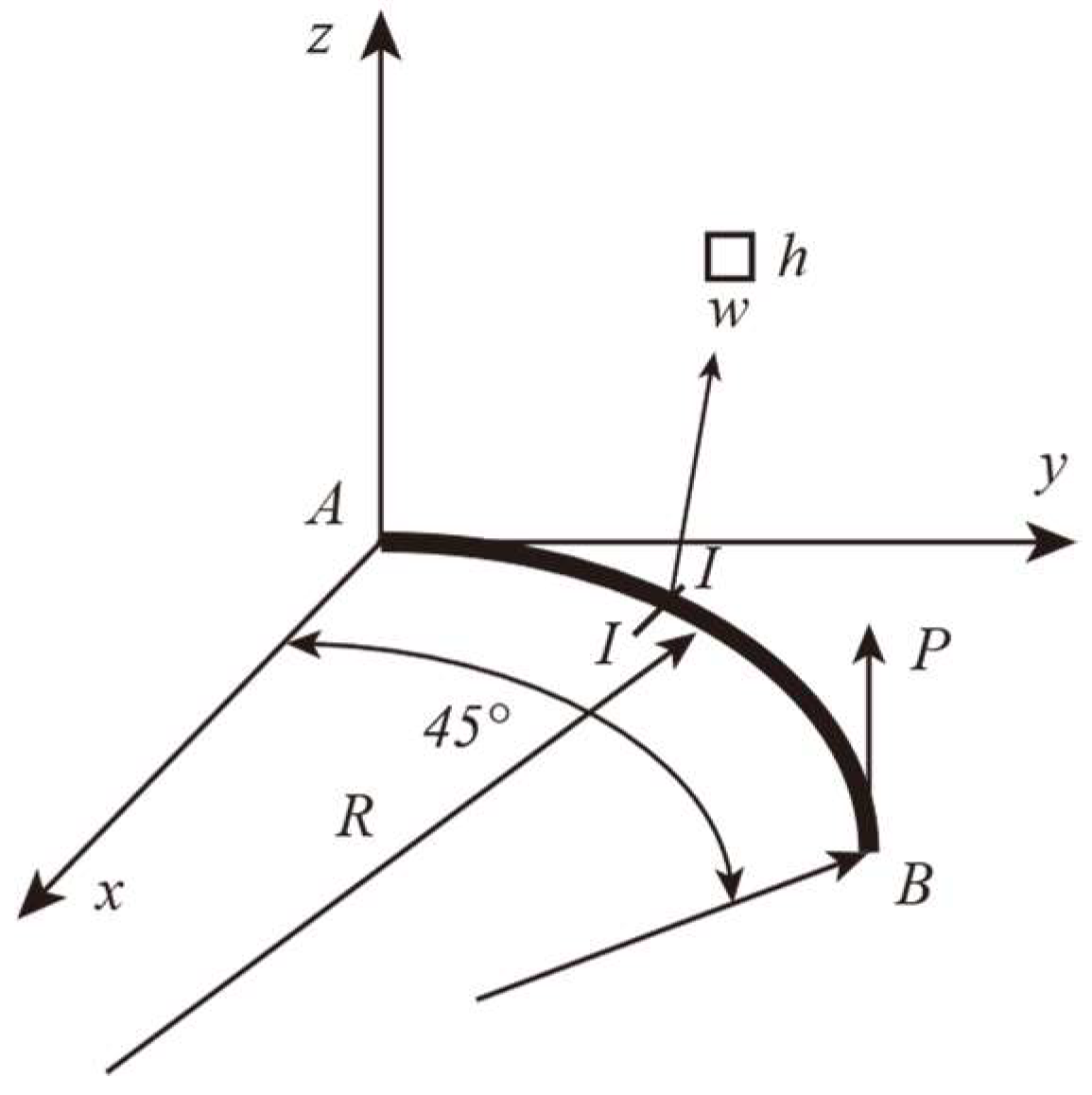
Example 4 illustrates the application of Beam3D element in dynamic time history analysis. A space curved beam (AB) is located in the $\mathrm{xoy}$ plane. End A is fixed, and end B is free, as shown in Figure 17. The center angle of the curved beam is 45°, with the radius of R = 100 in. The cross-section of the beam is a rectangle (width w= depth h = 1 in). Young’s modulus E is $1\times {10}^7\mathrm{psi}$, shear modulus G is $5\times {10}^6\mathrm{psi}$ and density $\rho$ is $2.54\times {10}^{-4}\mathrm{lb}·{\mathrm{s}}^2/{\mathrm{in}}^{-4}$. A concentrated load ($\mathrm{P}=300\mathrm{lb}$) perpendicular to the$\mathrm{xoy}$ plane is suddenly applied at the free end of the curve beam, and the duration is 0.3 s. The curved beam is simulated by 21 particles and 20 Beam3D elements. The time step $\mathsf{\Delta }t$ is taken as ${10}^{-5}\mathrm{s}$ to meet the stability of central difference, the analysis time t is 0.3 s and the damping coefficient $\alpha$ is taken as 0.

According to Chan’s study [60], the curved beam will vibrate under a suddenly applied load P. As shown in Figure 18, the openVFIFE results are compared with those of Chan’s study in which FEM was adopted. As can be seen, the openVFIFE results show reasonable agreements with the FEM results, especially in the z direction. This further validates that the Beam3D element as well as openVFIFE is effective in analyzing the dynamic nonlinear problems of space frames.

The above four examples verify the accuracy of the four structural elements (Link2DLD, Link3DLD, Beam2D and Beam3D) constructed in the present study. They also prove the ability of openVFIFE in structural behavior analysis, including but not limited to the following aspects: (1) static and dynamic analysis of structures; (2) nonlinear analysis of structures, including geometrical nonlinearity and material nonlinearity; (3) structural stability analysis.

5. Nonlinear Dynamic and Seismic Analysis of a Transmission Tower

Latticed transmission towers are important infrastructures and are major components of the power grid system. To illustrate the application of openVFIFE, dynamic nonlinear analyses of a latticed tower under sudden-applied and earthquake loads are conducted utilizing openVFIFE, respectively. The results are compared with that obtained from a commercial finite element software (ANSYS 19.0). All the examples are computed on a 64-bit Linux machine with an Intel Xeon E3-1230 v2 processor.

5.1. Model Establishment

A ±800kV double-circuit tangent transmission tower is studied. The elevation of the tower is depicted in Figure 19. The height of the tower body is 42 m, and its total height is 48.8 m. The sections of the tower columns are square, and the materials are equilateral angle steel, as listed in

Table 4. Material parameters of the transmission tower.

Material Type	Section Area (m2)	Terial Type	Section Area (m2)
L200 × 18	6.88 × 10−3	L90 × 7	1.21 × 10−3
L200 × 16	6.14 × 10−3	L80 × 7	1.07 × 10−3
L180 × 16	5.50 × 10−3	L80 × 6	9.24 × 10−4
L180 × 14	4.84 × 10−3	L75 × 6	8.64 × 10−4
L160 × 14	4.28 × 10−3	L75 × 5	7.25 × 10−4
L160 × 12	3.70 × 10−3	L70 × 5	6.75 × 10−4
L140 × 12	3.22 × 10−3	L63 × 5	6.05 × 10−4
L125 × 10	2.40 × 10−3	L56 × 5	5.35 × 10−4
L125 × 8	1.94 × 10−3	L56 × 4	4.32 × 10−4
L110 × 10	2.10 × 10−3	L50 × 4	3.84 × 10−4
L110 × 8	1.70 × 10−3	L45 × 4	3.44 × 10−4
L100 × 8	1.54 × 10−3	L40 × 4	3.04 × 10−4
L90 × 8	1.38 × 10−3

; the density of the material is 7850 kg/m³ and the Young’s modulus is 2.06 × 10¹¹ Pa. The models of VFIFE and FEM are established by openVFIFE and ANSYS software, respectively. The finite element model established in ANSYS adopts a Link180 element and a Beam188 element, and the VFIFE model established in openVFIFE adopts a Link3DLD element and a Beam3D element, as shown in Figure 20. As J.G.S. da Silva [61] pointed out, using truss elements (such as Link180 in ANSYS or Link3DLD in openVFIFE) to simulate the transmission tower will cause a lack of constraints at the transverse layer such that the tower will become a geometrically unstable system. To avoid this problem, the main materials and diagonal materials are simulated by the Link180 element in ANSYS and by the Link3DLD element in openVFIFE. The transverse materials are simulated by a Beam188 element and a Beam3D element in ANSYS and openVFIFE, respectively. The models in both ANSYS and openVFIFE consist of 191 nodes/particles and 569 elements.

As stated before, there is no need to integrate the global mass and stiffness matrix in VFIFE, so openVFIFE cannot conduct modal analysis of the tower. However, to understand the tower’s dynamic characteristics, the modal analysis is conducted in ANSYS. The natural frequencies of the first six order modes are listed in

Table 5. Natural tower frequencies.

Number of Order	Frequency/Hz	Mode
1	1.720	bending along x direction
2	1.831	bending along y direction
3	1.999	torsion around z direction
4	4.912	bending along x direction
5	8.785	bending of cross-arm
6	8.868	bending along x direction

.

5.2. Nonlinear Dynamic Analysis

Firstly, the dynamic behavior of a tower under suddenly applied loads is computed to compare the capabilities of FEM and VFIFE. A sudden load is applied to every node/particle of the model along the negative direction of the y-axis. The load remains at 0 N until time 0.1 s, then suddenly increases to 10,000 N and lasts for 59.9 s. The damping coefficient $\alpha$ is taken as 0.5 in both ANSYS and openVFIFE. In ANSYS, the full transient analysis is adopted, which uses an implicit integration method (Newmark-Beta) to solve the governing equations. Hence, the time step can be relatively large. In ANSYS, in order to ensure the stability of the integration algorithm, time step $\mathsf{\Delta }t$ is taken as ${10}^{-3}\mathrm{s}$ from 0.1 s to 1 s, and ${10}^{-2}\mathrm{s}$ from 1s to 60 s. In openVFIFE, the time step $\mathsf{\Delta }t$ is taken as ${10}^{-4}\mathrm{s}$. In addition, geometrical nonlinearity is considered in both ANSYS and openVFIFE.

Figure 21 shows the time history of the displacement of node/particle 47 (see Figure 20), and Figure 22 shows the displacements of every node/particle at $t=60$ s. It can be seen that the results of openVFIFE and ANSYS are almost the same. The mean displacements of node/particle 47 calculated by ANSYS and openVFIFE are 0.812 m and −0.805 m, respectively. Thus, the relative error is only −0.832%. Figure 23 shows the time history of the axial force of element 469 (see Figure 20), and the axial forces of every truss element (Link180/Link3DLD) at $t=60\mathrm{s}$ are plotted in Figure 24. It is clear that the internal force calculated by openVFIFE is accurate enough. To evaluate the accuracy of openVFIFE, the errors are computed by:

$$\begin{array}{c}\mathrm{error}=\frac{\Vert y_{ANSYS}-y_{openVFIFE}\Vert {}_1}{\Vert y_{ANSYS}\Vert {}_1}\end{array}$$

(14)

where $y_{ANSYS}$ and $y_{openVFIFE}$ are the result vectors calculated by ANSYS and openVFIFE, respectively. For instance, when calculating the error of node displacement, $y_{ANSYS}$ is taken as ${\left[y_1,y_2,\dots ,y_i,\dots y_n\right]}^T$ ($y_i$ is the displacement of node $\mathrm{i}$ calculated by ANSYS) and $y_{openVFIFE}$ is the taken as ${\left[y_1^{\prime },y_2^{\prime },\dots ,y_i^{\prime },\dots y_n^{\prime }\right]}^T$ ($y_i^{\prime }$ is the displacement of particle $i$ calculated by openVFIFE). The errors are listed in

Table 6. Errors of openVFIFE.

Item	Description	Error (%)
Node displacement	Uy1	0.009
Internal force of truss element	N1	0.077

¹Uy is displacement along the y-axis; N is axial force.

. It’s worth noting that it takes about 654.0 s to complete the analysis in ANSYS, while openVFIFE takes only 107.7 s. Clearly, the computing efficiency of openVFIFE is higher, largely because there is no iteration process in explicit integration.

5.3. Time-History Analysis under Earthquake

The acceleration time history of ground motion recorded in the El Centro earthquake [62] is selected when conducting the seismic analysis, as shown in Figure 25. The peak ground acceleration (PGA) is 0.2808 g (g is gravity acceleration), and the time interval of ground motion is 0.01 s. Therefore, to meet the stability of central difference, the time step of El Centro ground motion in FEM is taken as 0.01 s, while that taken in openVFIFE is 0.0001 s. The acceleration in openVFIFE is calculated by inputting the acceleration history using a linear interpolation method. The earthquake acceleration is inputted transversely to the transmission tower. The other computation parameters are same as in Section 5.2. The time history curves of the displacement of node/particle 47 are plotted in Figure 26, and those of the axial force of element 469 are plotted in Figure 27.

As can be seen in Figure 26 and Figure 27, the calculated responses of the transmission tower under earthquake acceleration obtained from ANSYS and openVFIFE almost coincide with each other. The maximum displacement at 5.26 s is 106 mm for the openVFIFE platform and 105 mm for ANSYS. The relative displacement error of particles is quite small. These results illustrate that the seismic time history analysis obtained from openVFIFE is reliable, and the efficiency of openVFIFE is proved again in the seismic analysis. It is worth mentioning that the computing times in ANSYS and openVFIFE are 1025.6 s and 108.2 s, respectively.

5.4. Collapse Analysis under Earthquake

In the past several decades, there are numerous instances of damages to the transmission towers due to earthquakes [63] or strong winds [64,65]. For example, more than 20 towers collapsed during the Wenchuan earthquake in 2008 [63]. There are two typical failure modes of transmission towers under strong earthquake: (1) tower top damages, (2) the whole tower tilts, as shown in Figure 28.

The simulation of the progressive collapse of a transmission tower under an extremely strong earthquake is complicated. The above examples strongly prove that the validity of the openVFIFE in static analysis, dynamic analysis and nonlinear analysis. However, as mentioned before, one of the advantages of VFIFE is its ability to analyze the discontinuous behavior of structures, which is hardly solved by FEM. The collapse analysis of the transmission tower under earthquakes has been conducted by openVFIFE to illustrate its application on discontinuous behavior analysis. The bilinear elastic-plastic constitutive damage model is adopted, as shown in Figure 29. The elastic modulus $E_e=2.06\times {10}^{11}\mathrm{Pa}$, plastic modulus $E_p=2.06\times {10}^{10}\mathrm{Pa}$, the initial yield stress ${\sigma }_y=2.35\times {10}^8\mathrm{Pa}$ and the ultimate strain ${\epsilon }_u=0.03$. If the strain of an element reaches the ultimate strain ${\epsilon }_u$, this element fractures and its internal force becomes zero. In order to make the transmission tower collapse, the acceleration of the earthquake ground motion is amplified 10 times, and the PGA reaches 2.808 g. Other calculation parameters are same as those used in Section 5.3.

The entire process of the collapse of the tower is shown in Figure 30. It is found that the tip of the cross-arm destroys first at about 33.2 s, which is similar to the failure mode shown in Figure 28a. At about 35.1 s, the failure of some elements at the diaphragm leads to the instability of the diaphragm at the bottom of the tower. The tower tilts evidently and loses its bearing capacity. From 35.1 s to 38.0 s, the tower continues to topple. But the tower legs still work. At about 38.8 s, the tower fully tilts, and the legs at the bottom of the tower fracture due to significant deformations. It is obvious that the failure of the tower is in good agreement with the failure mode shown in Figure 28b.

Figure 31 shows the evolution of the strains of the tower leg. It is clear that the element 512 fractures when its strain reaches the ultimate value 0.03, which is consistent with the defined ultimate strain for the tower material. It indicates that the present openVFIFE is effective in simulating the entire process of the collapse of structures.

6. Conclusions

VFIFE is a new structural analysis method that has significant advantages in the large deformation analysis, nonlinear dynamic analysis, discontinuous behavior analysis, etc., of a structure. It has therefore been widely used in civil engineering, marine engineering and mechanical engineering. To provide a general VFIFE analysis platform for researchers and engineers, an object-oriented general structural analysis platform (openVFIFE) based on VFIFE is developed in this paper. This platform is structured by a layered architecture with two layers: the controller and the core solver. In the core solver, four modules including particle class, element library, material library and section library are developed to implement the computing tasks of VFIFE. In the controller, a StructSystem class is achieved to manage objects created in the core solver and encapsulate the core solver. Six types of elements are implemented, including planar bar element (Link2D), space bar element (Link3D), flexibility planar bar element (Link2DLD), flexibility space bar element (Link3DLD), planar frame element (Beam2D) and space frame element (Beam3D). Three material models are achieved, including linear elastic material (LinearElastic), ideal elastoplastic material (UniIdeal) and bilinear elastoplastic material (UniBlinear). To validate the reliability and efficiency of the platform, a series of numerical examples are conducted. Furthermore, to extend the applications of VFIFE, the nonlinear dynamic and collapse process of a transmission tower under earthquake load are studied using openVFIFE.

Based on the numerical results presented in this paper, the following conclusions can be drawn:

• The accuracy of elements and material models in openVFIFE are verified by four numerical examples. The capacity of the platform in large deformation analysis, elastic-plastic analysis and nonlinear dynamic analysis is also confirmed by these numerical examples.
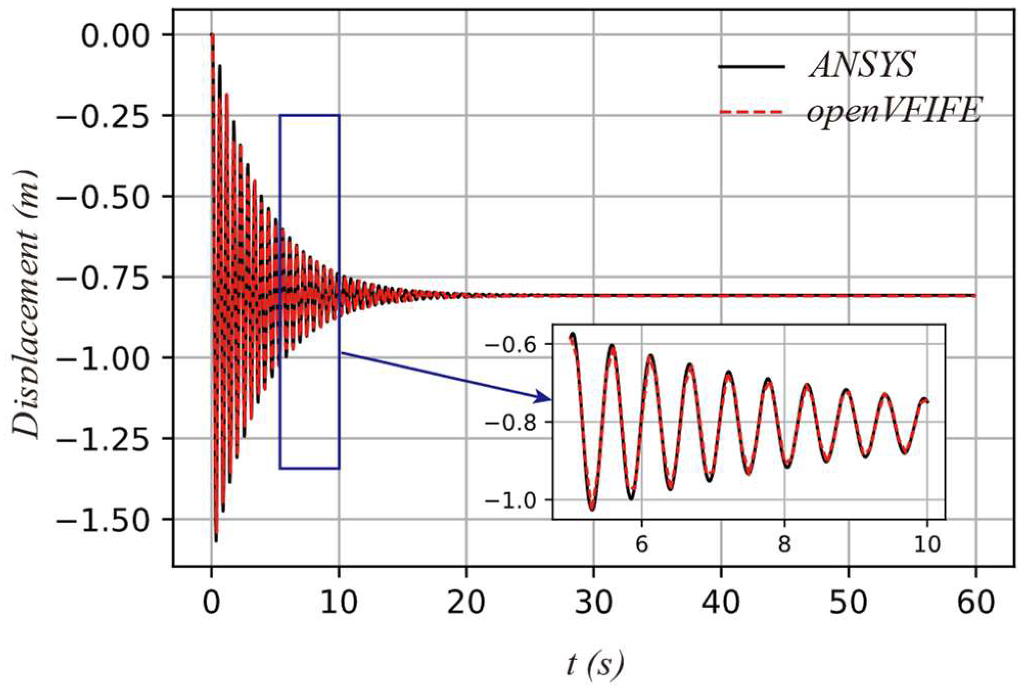
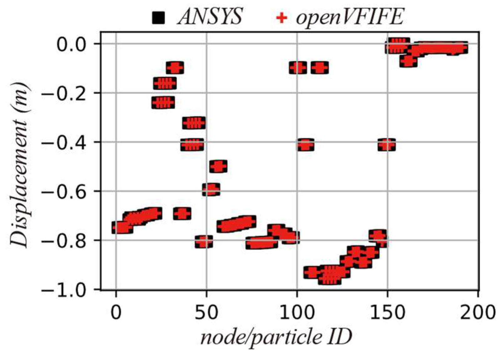
• Benefiting from the explicit solution strategy and the well-designed object-oriented framework, the proposed platform is much more efficient than ANSYS in nonlinear dynamic analysis. Its operation speed is about 6–10 times faster than ANSYS.
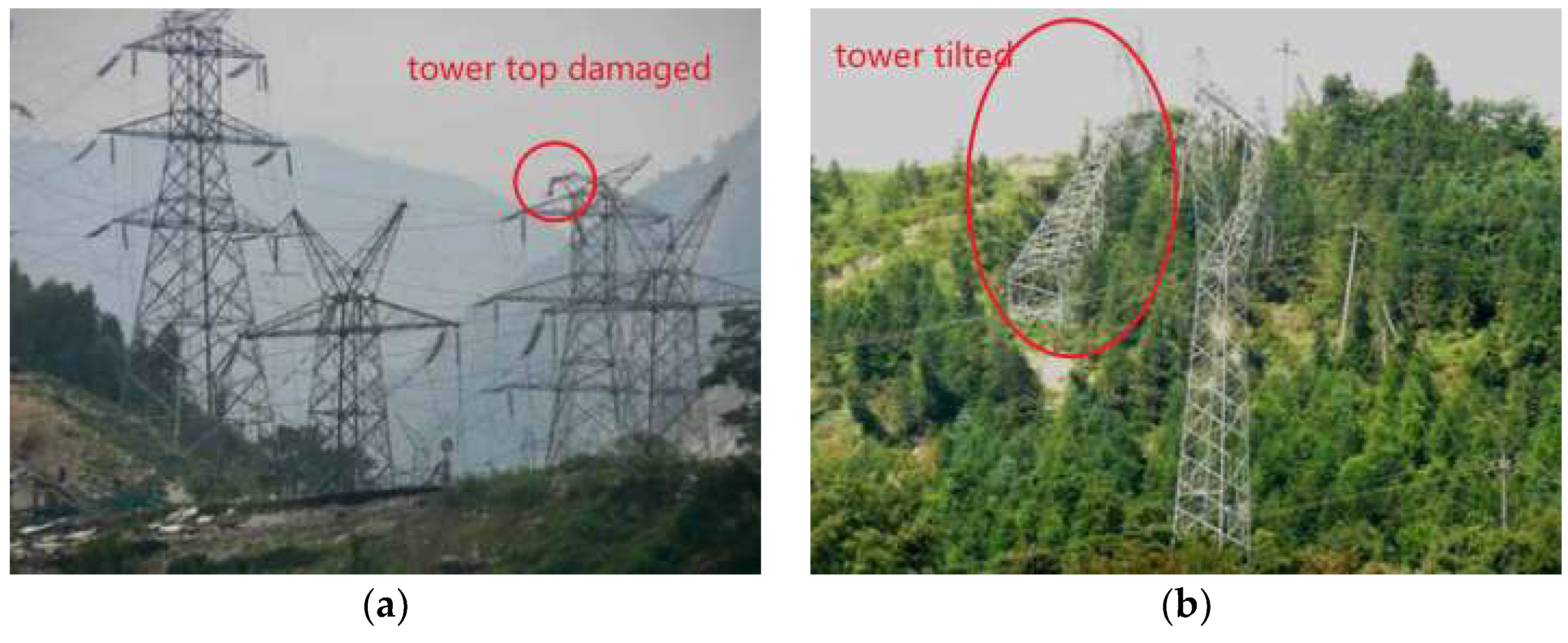
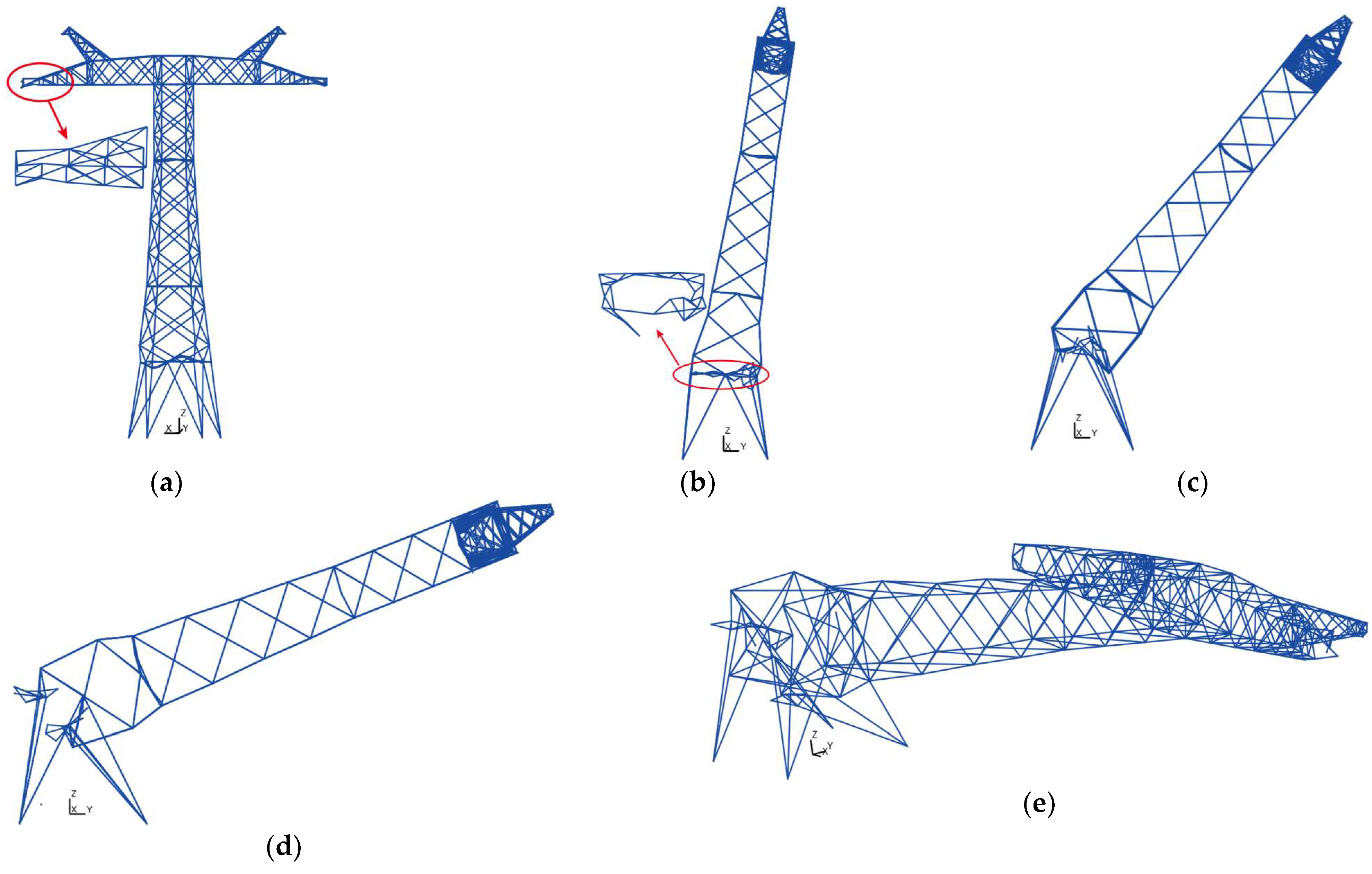
• In addition, the entire-process collapse of the transmission tower under earthquake loads has been successfully simulated by the openVFIFE. Firstly, the cross-arm of the tower destroys, and then the whole tower tilts under a strong earthquake, which is consistent with the failure modes observed in real cases. The study lays the foundation for further investigation of the collapse mechanism, failure modes and their control of the transmission towers.