1. Introduction
Wind-driven rain (WDR), referring to raindrops carried by wind and deposited on building façades, influences the hygrothermal performance and durability of building façades significantly. Zones of the building envelope exposed to higher amounts of rain usually show a higher risk of moisture-related deterioration. Deterioration of building materials due to WDR is a significant issue when retrofitting old or historical buildings. Additionally, WDR load is often a critical boundary condition in studies of hygrothermal transport in building envelopes, relating moisture damage risk to rain absorption into porous building materials and to leakage into façades [
1]. Therefore, a significant amount of WDR research focuses on the quantification of WDR intensity on building façades [
2].
Moisture accumulation in building envelopes can increase the risk of moisture-related degradation such as mold growth or wood decay, and freeze–thaw damage, among others. Vandemeulebroucke et al. [
3] grouped indices that evaluate the risk of moisture-induced damage in two broad categories: climate-based indices, and response-based indices. Climate-based indices include those that can be calculated based on meteorological data, e.g., climatic index [
1], moisture index [
4], number of freeze–thaw cycles based on air temperature [
5], time of frost [
6], and wet frost [
7]. Response-based indices require hygrothermal simulations of the building envelope response and post-processing of the simulation data, e.g., mold index [
8], RHT index [
9], and critical freeze–thaw cycles [
10,
11]. Recently, Zhou et al. [
12] proposed a new freeze–thaw damage risk (FTDR) index by simulating actual ice growth and melt cycles, taking into account the effect of ice content difference over the number of freeze–thaw cycles. Using such indices, several studies investigated moisture-induced damage risks and durability, taking into account climate change based on predicted future conditions [
3,
5,
13,
14,
15]. Time-varying data for future conditions can be obtained by combining current observations from a weather station with climate projections by “weather morphing” [
14,
16], or directly from the output of regional climate models [
15,
17].
In order to evaluate moisture-induced damage risks, it is common to perform one-dimensional hygrothermal simulations of building envelope assemblies to assess their long-term performance [
1]. While this approach resolves the moisture transport in the actual structure of building envelopes, WDR load is mostly simplified by the use of semi-empirical models, which are prone to deficiencies and large uncertainties, unable to capture the effects of local wind-flow features correctly, and defined only for a limited number of common building geometries [
18,
19,
20]. In reality, WDR exposure over actual three-dimensional building envelopes can be locally much smaller or larger. Towards a conservative assessment of possible leakage and moisture damage, zones with large WDR exposure should be identified and analyzed.
Climate-based indices can be used as fast methods to provide an initial estimate of the level of risk of moisture-induced damage, and to assess the severity of current and future climatic conditions without hygrothermal simulations. The “climatic index” [
1], based on annual amounts of wetting and drying, is appropriate for such purposes. Annual wetting load is estimated by semi-empirical models for WDR, and annual drying is estimated by potential evaporation. In the present study, we build upon this approach by resolving the distribution of WDR load with the help of computational fluid dynamics (CFD) simulations. CFD simulations are used to obtain the detailed distribution of surface wetting due to WDR, using a validated Eulerian multiphase model.
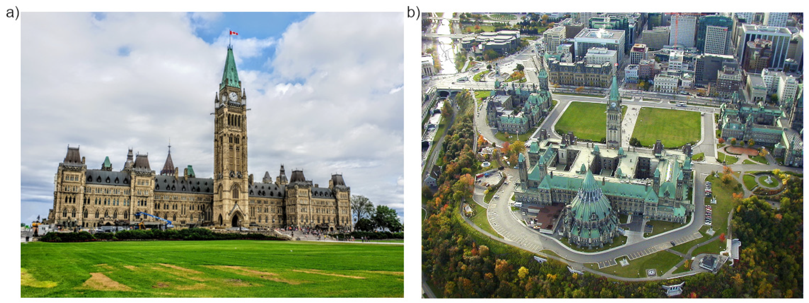
The case study is the Canadian Parliament buildings—located on Parliament Hill, Ottawa, Canada—which consist of a group of historical buildings with high significance for cultural heritage. Currently, the Parliament buildings are under restoration as part of a long-term project, which includes the addition of interior insulation to increase energy efficiency. This modification to the building envelope could increase the risk of freeze–thaw cycles. In order to correctly evaluate the related freeze–thaw damage risk, an accurate prediction of WDR load is of utmost importance. The buildings have complex geometry, including towers, façade detailing, and abundant modulations (
Figure 1), and they are surrounded by several other buildings. Such complex building features may yield possible locations of high WDR exposure. The buildings are located on an escarpment, which can further increase the WDR exposure. This case study is particularly interesting considering the impact of climate change, which is predicted to increase the total amount of rainfall in Ottawa. The results may help with identifying future risk areas, and with preventive maintenance. Long-term WDR exposure is then compared with potential evaporation, which is a measure of the ability of the environment to remove water at the surface of the building envelope. The orientation of a building façade and the particular position on the façade can strongly affect WDR exposure and drying rate. For example, a location can have a high exposure to WDR but a lower drying rate due to low exposure to solar radiation, leading to moisture residing within the envelope for a longer duration.
The aims of the study are (1) to present a fast methodology allowing the determination of the critical locations on the façades of complex buildings that are prone to higher moisture damage risks, taking into account their actual built environment; (2) to perform a fast assessment of the critical periods for moisture-induced damage risks; and (3) to evaluate the current and future moisture damage risks, particularly in terms of freeze–thaw damage. The remainder of the paper is organized as follows:
Section 2 explains the numerical model for WDR simulations and for evaluating potential evaporation.
Section 3 describes the computational domain and grid for the case study.
Section 4 presents the meteorological conditions obtained from a local weather station.
Section 5 describes the boundary conditions for the simulations.
Section 6 presents the results of surface wetting due to WDR, compares the annual wetting load with potential evaporation, and discusses the potential impact of climate change. Finally,
Section 7 and
Section 8 provide discussion on the obtained results and conclusions.
2. Methodology
2.1. Numerical Modeling of Wind-Driven Rain
2.1.1. Governing Equations
WDR intensity on building surfaces is calculated based on steady-state simulations of wind flow and rain. Steady Reynolds-averaged Navier–Stokes (RANS) CFD simulations are used to calculate the incompressible wind-flow field with the realizable k-ε turbulence model [
23]. The calculated wind-flow field is used to drive the raindrops in the rain simulations, for which a validated Eulerian multiphase model is used [
24,
25,
26,
27]. One-way coupling between raindrops and wind-flow field is used, ignoring the effect of raindrops on the wind flow.
Rain is modeled as a continuum, and separate rain phases are defined for classes of raindrop size, corresponding to a range of droplet diameters that show similar WDR behavior. The following continuity and momentum equations are solved separately for each rain phase, instead of tracking individual raindrops:
where
d denotes the raindrop diameter,
αd the phase fraction of the rain phase with diameter
d,
ud,j the velocity component of the rain phase,
ui the velocity component of wind,
ρw the density of water,
μa the dynamic viscosity of air,
gi the gravitational acceleration, and
Cd the drag coefficient. The overbar denotes Reynolds averaging. The terms on the left-hand side in Equation (2) are the mean convective flux and the turbulent flux. The terms on the right-hand side represent the gravity and the drag forces. Drag coefficients are obtained based on the measurements of terminal velocities of free-falling water droplets by Gunn and Kinzer [
28]. Re
R denotes the relative Reynolds number calculated using the relative velocity between the air and rain phases. The turbulent dispersion of raindrops is taken into account by the second term on the left-hand side in Equation (2). This term is modeled by defining a response coefficient based on the particle relaxation time, which is the rate of response of particle acceleration to the relative velocity between the particle and the carrier fluid, and the Lagrangian fluid time scale, which is the characteristic large eddy lifetime [
29].
The numerical model for WDR is implemented into a solver based on OpenFOAM v6 (download available, windDrivenRainFoam [
30]), and has been validated in numerous studies [
25,
26,
27].
2.1.2. Distribution of Wind-Driven Rain Intensity
One of the advantages of modeling rain as a continuum, rather than considering individual raindrops with particle tracking methods, is that the WDR intensity can be calculated everywhere in the computational domain based on the distribution of rain phase fraction and rain velocity. This is particularly beneficial for complex building shapes with small façade detailing, which are not accounted for in available semi-empirical models.
From the calculated rain phase fraction and velocity, first, the spatial distributions of “specific catch ratio”,
ηd, are obtained separately. Specific catch ratio indicates the non-dimensional WDR intensity due to a specific raindrop size, normalized by the horizontal rainfall intensity. Then, the catch ratio,
η, representing wetting due to the complete spectrum of raindrops, can be calculated on each location on the building as follows:
where
Rwdr denotes the WDR intensity,
Rh the horizontal rain intensity through the horizontal plane, and
fh(
Rh,
d) the raindrop size distribution [
31] through the horizontal plane at rain intensity
Rh. Note that the catch ratio provides the amount of rain deposition but, once deposited, further interactions between the raindrops and the walls are not modeled. Hence, neither the raindrop physics after impinging nor the surface film runoff are considered.
Catch ratio is influenced by meteorological conditions such as wind speed, wind direction, and rainfall intensity, as well as building geometry and local wind-flow features such as wind recirculation zones, wind sheltering, and wind acceleration. Such local wind-flow patterns are directly taken into account by the applied CFD approach, while semi-empirical models would need additional parameters and elaborate calibration [
32,
33].
The present approach creates a database of spatial distributions of catch ratio for a range of values of reference wind direction, wind speed, and rainfall intensity, based on the calculated rain velocity and rain phase fraction. Then, the catch ratio values can be interpolated considering the local meteorological data in order to obtain the temporal variation of surface wetting on buildings [
34].
2.2. Potential Evaporation and the Climatic Index
To obtain a drying index, the potential evaporation on a vertical surface based on the Penman equation [
35,
36] is used. This approach is widely used in the fields of agricultural and environmental physics for predicting the potential evaporation from a surface. Similar to the wetting distribution, this approach also considers the influence of façade orientation, while taking into account meteorological factors such as air temperature, air humidity, wind speed, short-wave solar radiation, and long-wave radiation. For the calculation of potential evaporation, the corresponding values obtained from the weather station are used.
The potential evaporation (
PE) from a vertical surface can be obtained as follows [
1]:
where Δ denotes the gradient between saturation vapor partial pressure and air temperature,
γ the psychrometric constant,
K the net short-wave radiation,
L the net long-wave radiation,
I the latent heat of vaporization,
hm the convective vapor transfer coefficient,
ea the saturation vapor partial pressure in the air, and
e the vapor partial pressure in the air. The first term on the right-hand side in Equation (4) deals with the radiative energy balance at the surface, while the second term deals with the atmospheric convective conditions. For further details on how PE is calculated, we refer to Zhou et al. [
1].
The climatic index is defined as the ratio between the annual wetting load and annual drying potential [
1]. The WDR load is obtained from the CFD simulations as described in
Section 2.1. For the climatic index, both the annual wetting load and the annual potential evaporation are calculated as the sum of hourly values. A higher climatic index value corresponds to a higher moisture risk for the building envelope. In the following sections, annual climatic index values will be calculated over several years. Furthermore, the cumulative WDR load will be compared to the cumulative potential evaporation to discuss critical periods in each year in more detail.
3. Description of the Case Study
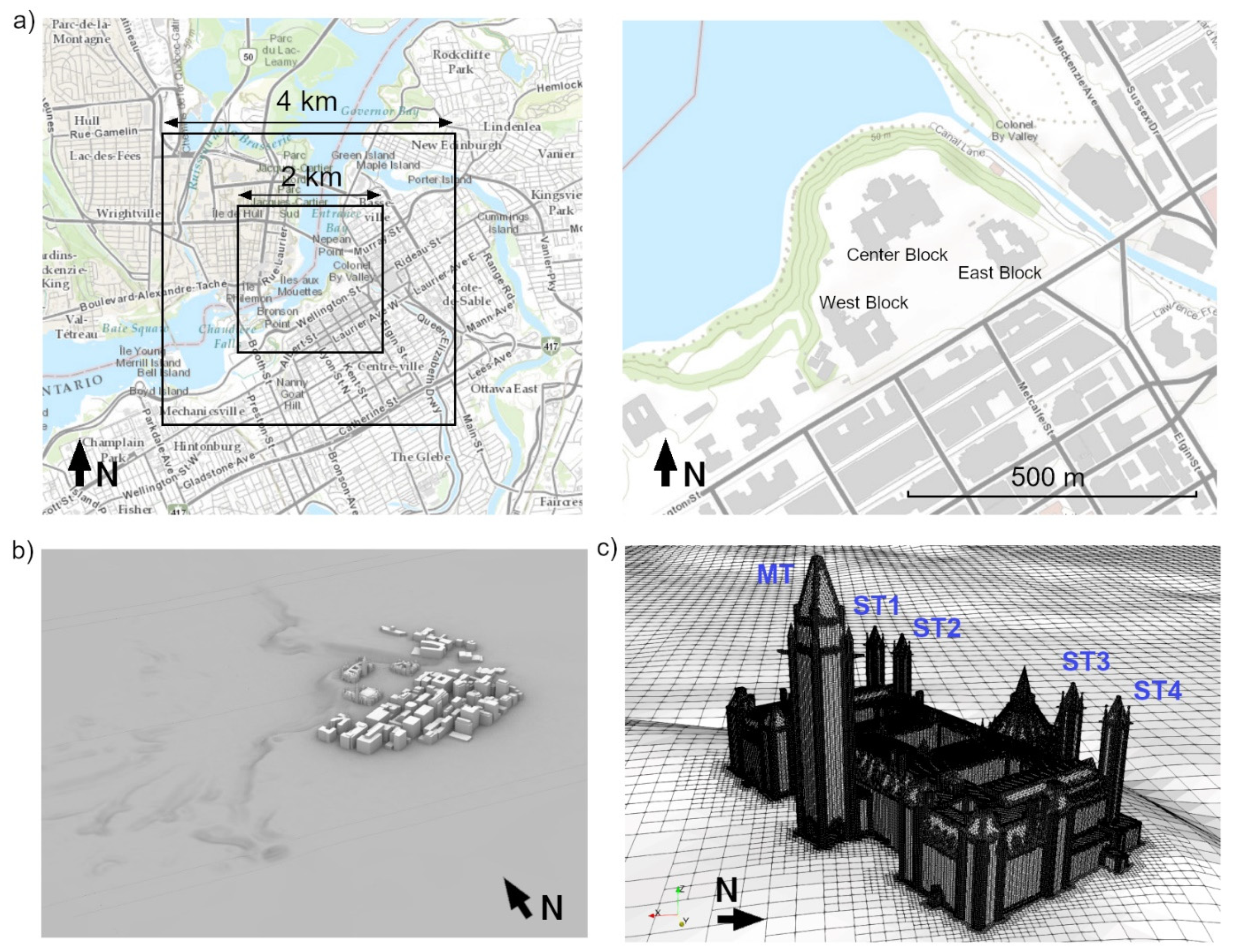
The Parliament buildings consist of three blocks—the Center Block, East Block, and West Block—which are located on a cliff with a steep escarpment descending to the Ottawa River to the north and west, and to the Rideau Canal to the east. The total extent of the computational domain with a size of 4 × 4 km
2 is shown in
Figure 2a. The inner part with the dimensions of 2 × 2 km
2 accurately represents the terrain—particularly the elevation around Parliament Hill. The terrain within the outer part was smoothened towards the lateral domain boundaries in order to limit rapid changes in the flow direction. Point clouds for the terrain were obtained based on LiDAR measurement data owned by the City of Ottawa and accessible through Carleton University [
37].
Immediately to the south and southwest of the area, there is a relatively dense group of high-rise buildings. To the east, across the canal, lies a mixture of high-rise and low-rise buildings. To the north and northwest, buildings are located further away due to the presence of the river. The computational domain for the CFD simulations is given in
Figure 2b, which shows the explicitly modeled buildings and terrain. The buildings within a distance of 500 m from Parliament Hill were explicitly modeled. This is a larger distance than required in the guidelines of the City of London for urban wind-flow simulations [
38]. As shown in
Figure 2b, high-rise buildings located to the south are included, as well as a few buildings on the eastern side of the canal. No other buildings are included in the remaining directions, as a large part is covered by the river. The buildings remaining further than the distance of 500 m were not modeled directly, but their effects were imposed as ground roughness. The distances of buildings from domain boundaries and the blockage ratio of buildings satisfy the guidelines stated in Franke et al. [
39].
Part of the computational grid on the surfaces around the Center Block is shown in
Figure 2c. The computational grid was generated in two steps: In the first step, a terrain-following structured grid with uniform hexahedral cells was created without the buildings, using the meshing tool “gSurf” provided by Azevedo [
40]. The inputs for this tool are the point-cloud data for the terrain. The obtained grid was then used, in the second step, as an input for the OpenFOAM meshing tool “snappyHexMesh”, which creates the building-fitted grid. The resulting computational grid has a total of around 7.7 million cells, mostly hexahedral.
This study focuses on the Center Block, which is composed of the main building with a height of around 25 m, the main tower (MT) on the southern side with a height of around 92 m, and four smaller towers (ST1-ST4) on the northern side with a height of around 48 m (
Figure 2c). The building model includes the shape of the roof and façade detailing (Model by Disura on SketchUp 3D Warehouse [
41]). Past research shows a significant influence of roof overhangs, façade detailing, modulations such as window sills [
42], and recessed parts of the façade [
43] on WDR intensity. The applied Eulerian multiphase model is especially convenient for geometries with such fine details, as it quantifies the WDR intensity on all surfaces in the computational domain.
4. Meteorological Data
Weather data were collected from the OTTAWA CDA RCS weather station (Climate ID: 6105978), which is located in an open field approximately 4.5 km south–southwest of Parliament Hill. The retrieved data included dry-bulb temperature, wind speed, wind direction, relative humidity, precipitation, and rainfall, among others.
Rainfall was measured with tipping bucket gauges, and was only recorded during the warm season, roughly from April to October, in hourly intervals. Precipitation was measured with weighing gauges, which cannot differentiate between snow and rain, but are available in 15 min intervals throughout the year. The shorter 15 min data provide a higher accuracy for the CFD simulations of WDR compared to hourly data, as the hourly data will typically lead to a lower rainfall intensity, which would correspond to a different distribution of raindrop sizes in the air. Therefore, precipitation values are used in the present study, and precipitation in the form of snow is filtered out based on the measured air temperature.
Correction of the few missing/erroneous data on precipitation was performed by cross-comparing against the available daily values, which are quality controlled. Since the remaining data are also only available in hourly intervals, it was assumed that they remain constant during each hour. In terms of the hourly wind speed and wind direction, no additional post-processing or weighting was performed. Solar radiation data were obtained from the Canadian Weather Energy and Engineering Datasets (CWEEDS) from Ottawa International Airport station.
An analysis of the measured weather data was performed to determine the meteorological conditions during rain.
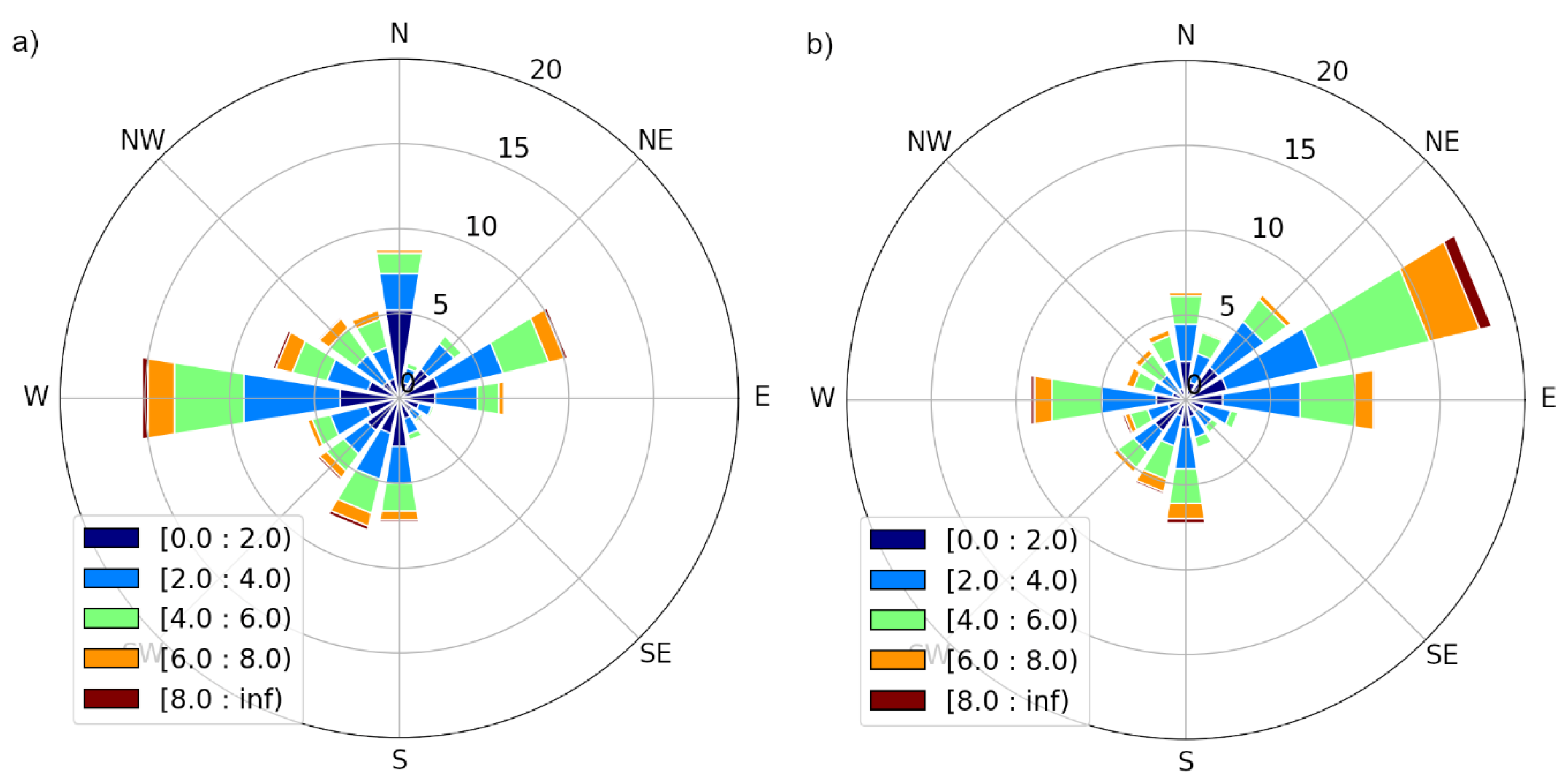
Figure 3a shows the wind rose for the weather data measured in the years 2010–2020. The primary wind direction is observed to be westerly, with relatively frequent winds also from the south and the east. When only the periods of rainfall are considered (
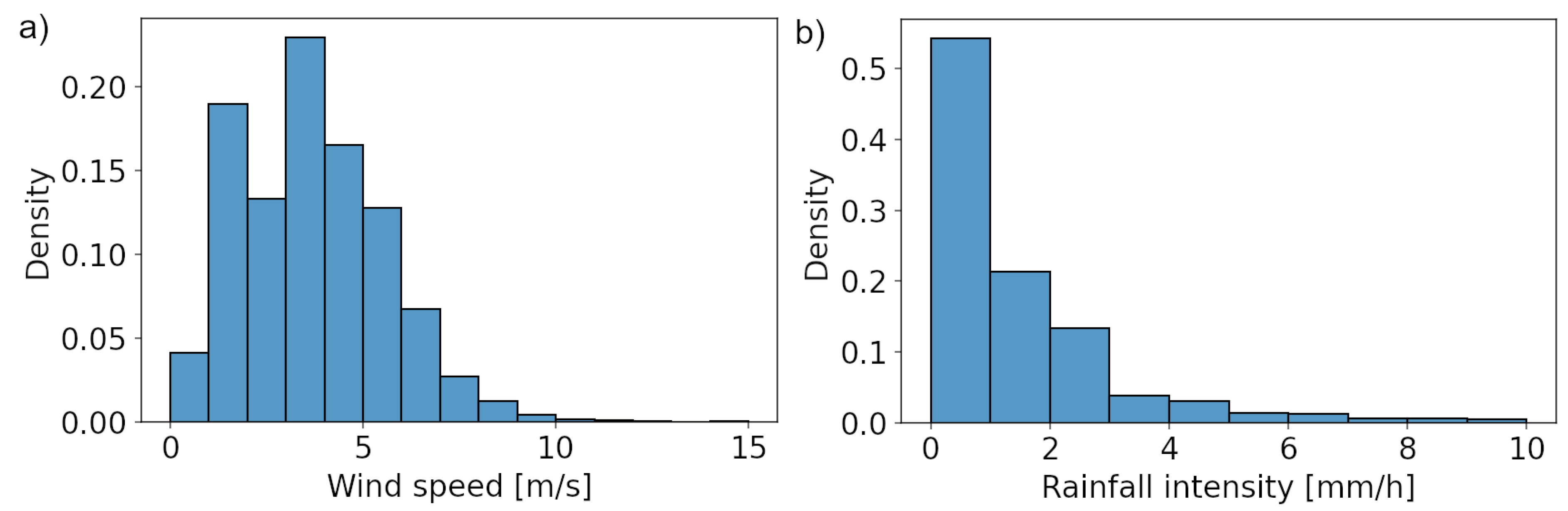
Figure 3b), wind from the east becomes significantly more recurrent in terms of both overall frequency and the number of events with high wind speeds. The histograms of rainfall intensity and wind speed during the periods of rainfall are provided in
Figure 4. The average rain intensity is 1.9 mm/h, representing light rain, and the average wind speed during rain is 3.7 m/s.
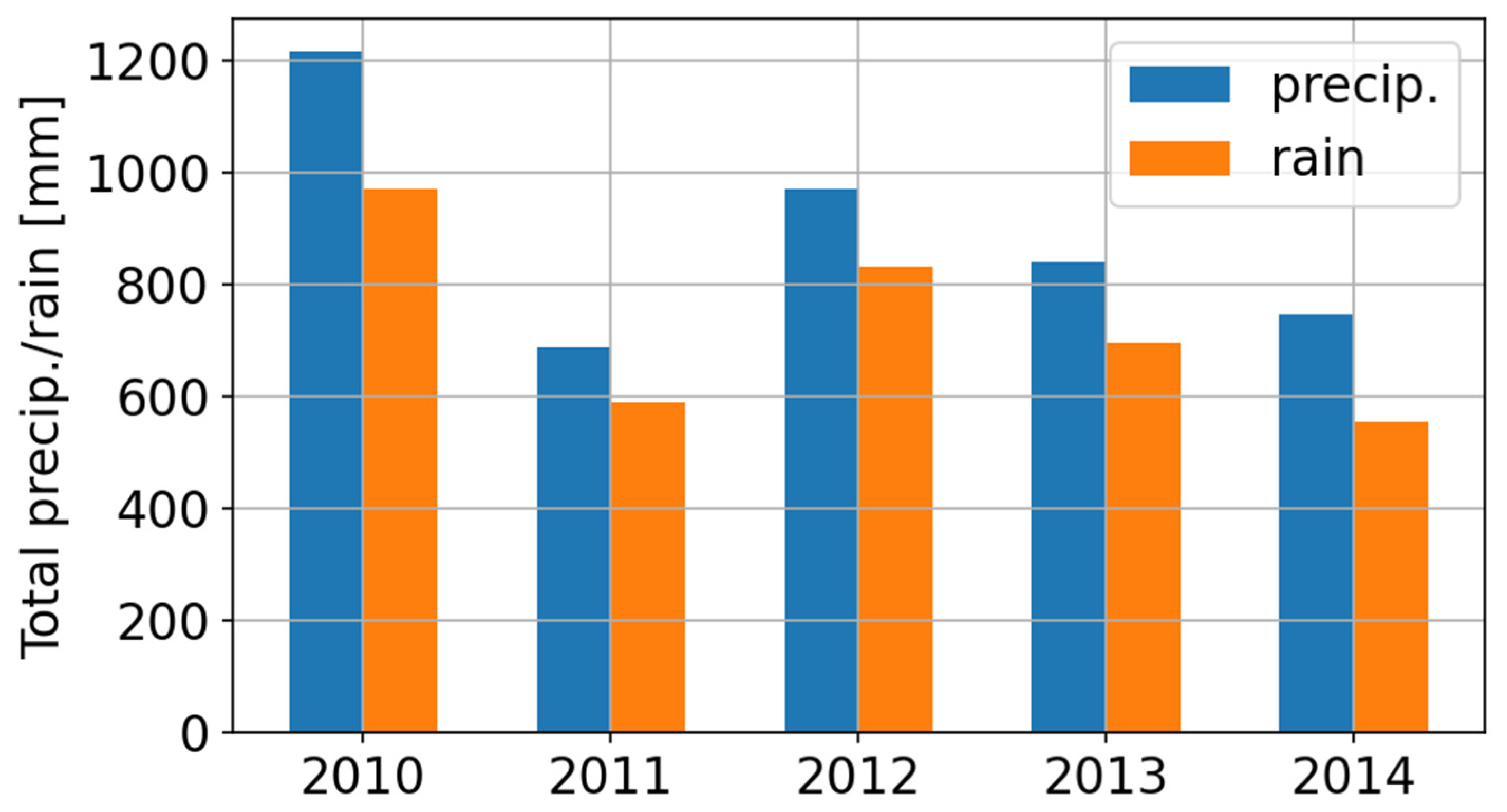
The total amounts of precipitation and rainfall are compared in
Figure 5 for several years, indicating that the amount of snowfall is around 18% of the total precipitation on average. The annual rainfall amount varies between 550 and 970 mm. Note that, here and in the remainder of the paper, each year starts in October and ends in September of the following year, in order to include a continuous wet season in the analyses. While the weather station data cover the period 2010–2020, the solar radiation data only partially overlap with the same period. Therefore, the analyses are presented between 2010 and 2014, i.e., October 2010–September 2015.
5. Numerical Settings
The numerical simulations of wind and rain were performed for eight wind directions in 45° increments, i.e., the cardinal and intercardinal directions. Steady wind-flow field was calculated for a reference wind speed of 10 m/s. Wind-flow fields for the remaining reference wind speeds were obtained by scaling the wind-velocity field from the calculated case [
25,
26] in order to cover the complete range of measured values. For each wind speed, the rain phase calculations were performed for 17 raindrop sizes ranging from 0.3 to 6 mm. From these, the catch ratio distributions were calculated for a range of reference rainfall intensities between 0.1 and 30 mm/h. The main settings of the simulation are given below, and more details can be found in [
45].
5.1. Boundary Conditions for Wind-Flow Simulations
For wind simulations, the inlet and outlet boundaries are defined based on the wind direction, i.e., for a wind direction of southwest, domain boundaries at the south and the west are defined as inlets. The atmospheric boundary layer profile at the inlet(s) is based on the log-law relation considering neutral conditions during rainfall. Vertical profiles of wind velocity
U, turbulence kinetic energy
k, and turbulence dissipation rate
ε are given below [
46]:
where
z denotes the height above the ground,
the atmospheric boundary layer (ABL) friction velocity,
κ the von Karman constant,
z0 the aerodynamic roughness length, and
Cμ a model constant. The aerodynamic roughness length at the inlet reflects the roughness conditions of a fetch of 5 km upstream of the inlet. At the outlet(s) boundary, a constant static gauge pressure of 0 Pa is set. The boundary condition for the top boundary is set as free slip.
For the building surfaces and the ground, standard wall functions are used. Building surfaces are assumed to be smooth and, for the ground surface, wall functions with surface roughness modifications are used.
5.2. Boundary Conditions for Rain Simulations
For the rain phases, inlet boundaries are defined as the boundaries from which rain enters the computational domain, i.e., the same inlet boundaries for the wind phase and, additionally, the top boundary. For these boundaries, the values of rain velocity and rain phase fraction need to be set.
The vertical component of rain velocity at the inlet is set to be equal to the terminal velocity for the corresponding raindrop size. As for the horizontal component of rain velocity, a fully developed profile is obtained by using a “pseudo-periodic condition” at the inlet: a recycling plane is defined, located 5 m downstream of the inlet plane, and the velocity values at the recycling plane are imposed back at the inlet plane. The resulting rain velocity profile is different for each raindrop size depending on the local force equilibrium between the inertia of raindrops and the drag force due to wind. The rain phase fraction at the inlet is given as:
where
Vt(
d) represents the terminal velocity of a raindrop with diameter
d.
At wall surfaces—i.e., buildings and ground—raindrops are modeled to leave the domain as soon as they hit the surface. This is achieved by setting the gradients of the rain fraction and rain velocity normal to the surface—∂αd/∂n and ∂ud/∂n, respectively—to zero. In case of a local backflow—i.e., rain velocity vector is pointing into the domain—the rain fraction value is set to zero.
6. Results
6.1. Surface Wetting Due to WDR
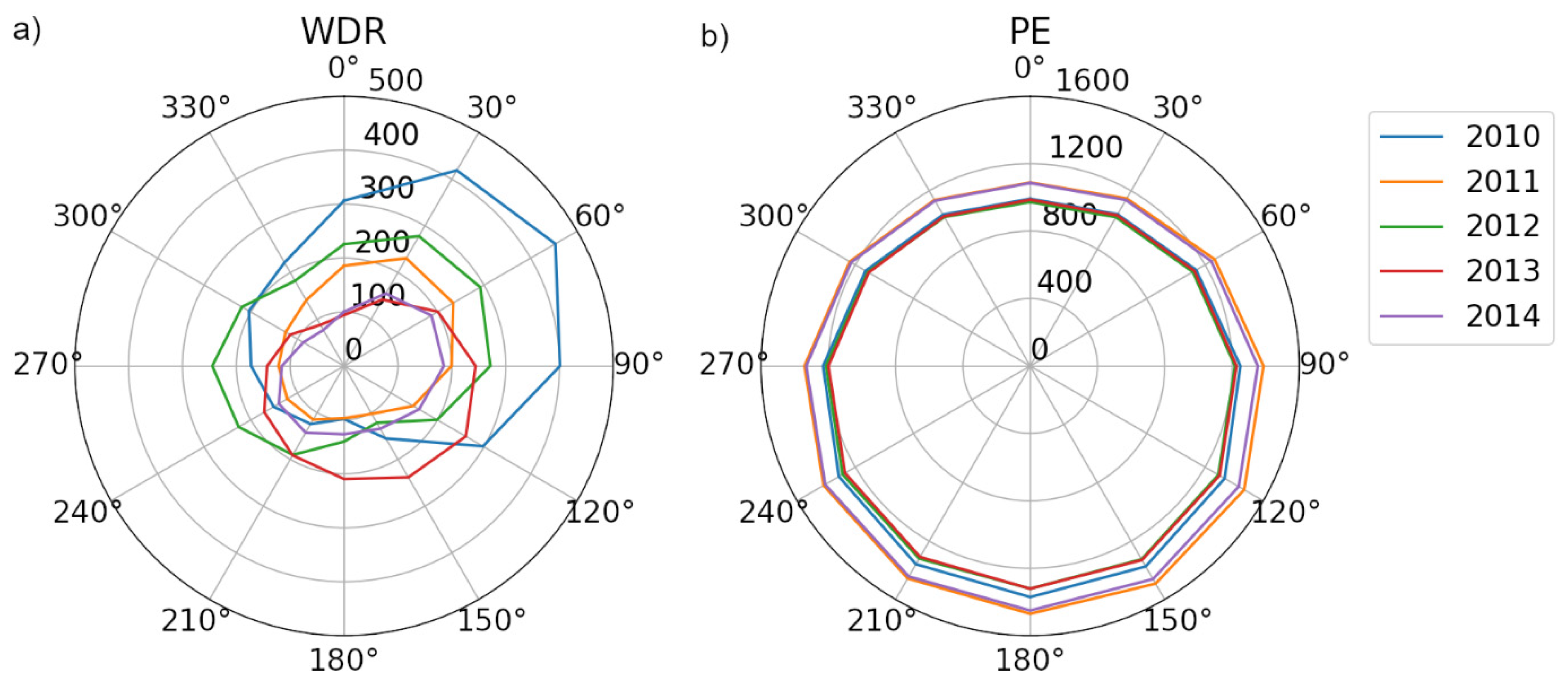
Figure 6a presents the free-field WDR amount—i.e., without the effect of buildings—for different orientations for the wetting periods in the years 2010–2014. Note that the free-field WDR is calculated using the relationship in Equation (9) [
47], where wind speed
U and rainfall intensity
Rh are the measured values,
θ being the angle between wind direction and orientation on the horizontal plane. The WDR coefficient
κ for the free-field conditions was taken as 0.222 [
48]. In 2010, a larger WDR exposure is observed from east–northeast, indicating the impact of the high-wind-speed events, which is also visible in the wind rose shown in
Figure 3b. The other years show a more balanced distribution with higher values from the east, northeast, southwest and south. Unlike the high variation in WDR each year, the potential evaporation given in
Figure 6b is more balanced across the five years, with slightly higher values in 2011 and 2014. Potential evaporation is highest in the southern directions (S/SSE/SSW) and lowest in the northern directions (N/NNW/NNE), mainly explained by the amounts of solar irradiation on vertical surfaces facing these directions. Note that the potential evaporation only differs per orientation, and does not depend on location on the building façade, i.e., local differences in terms of shadowing, air temperature, and heat/mass transfer coefficients are here ignored.
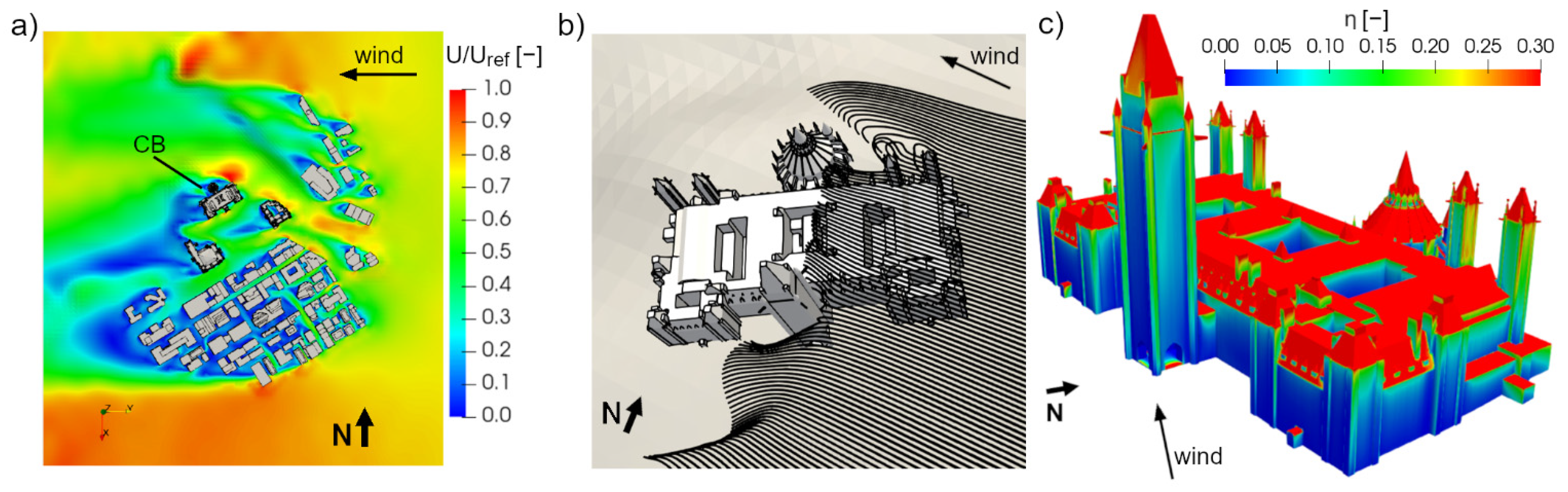
Figure 7a shows the normalized contours of wind speed for wind approaching from east. The resulting raindrop trajectories for raindrops of 1 mm diameter and the distribution of catch ratio on the Center Block surfaces are given in
Figure 7b,c, respectively, for a reference wind speed of 10 m/s and a rainfall intensity of 1 mm/h. Excluding roof surfaces, the highest WDR exposure is visible on the higher parts and corners of the façades—particularly on the eastern façades of the main and smaller towers.
The smaller towers have a significantly lower impact on the approaching wind flow, while the main tower causes a larger disturbance on the approaching wind flow, i.e., larger wind blockage. As a result, a significant part of the raindrops approaching the main tower are directed elsewhere around the corners, and higher catch ratio values are observed mainly near the side edges and the top part of the main tower. In contrast, smaller towers show higher catch ratios over a larger part of their eastern façade.
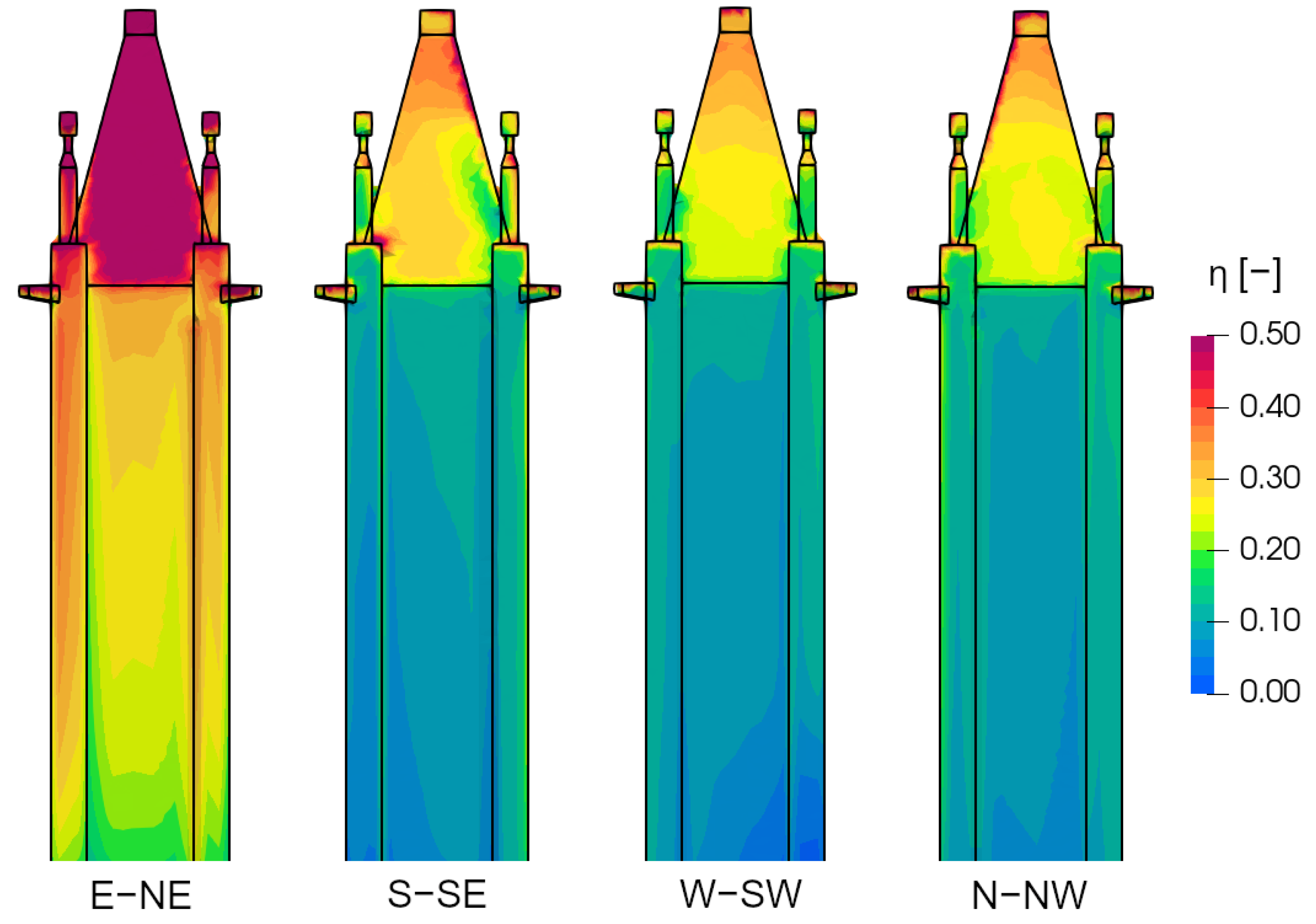
Figure 8 presents the catch ratio values for the year 2010 on all façades of the smaller tower #2. Here, the catch ratio is calculated as the total amount of WDR between October 2010 and September 2011 divided by the total amount of rainfall during the same period. The period between October 2010 and September 2011 was chosen because
Figure 6 indicates that this period is expected to be more severe, showing the highest values of free-field WDR for a large number of orientations and lower values for potential evaporation.
6.2. Comparison of Surface Wetting and Potential Evaporation
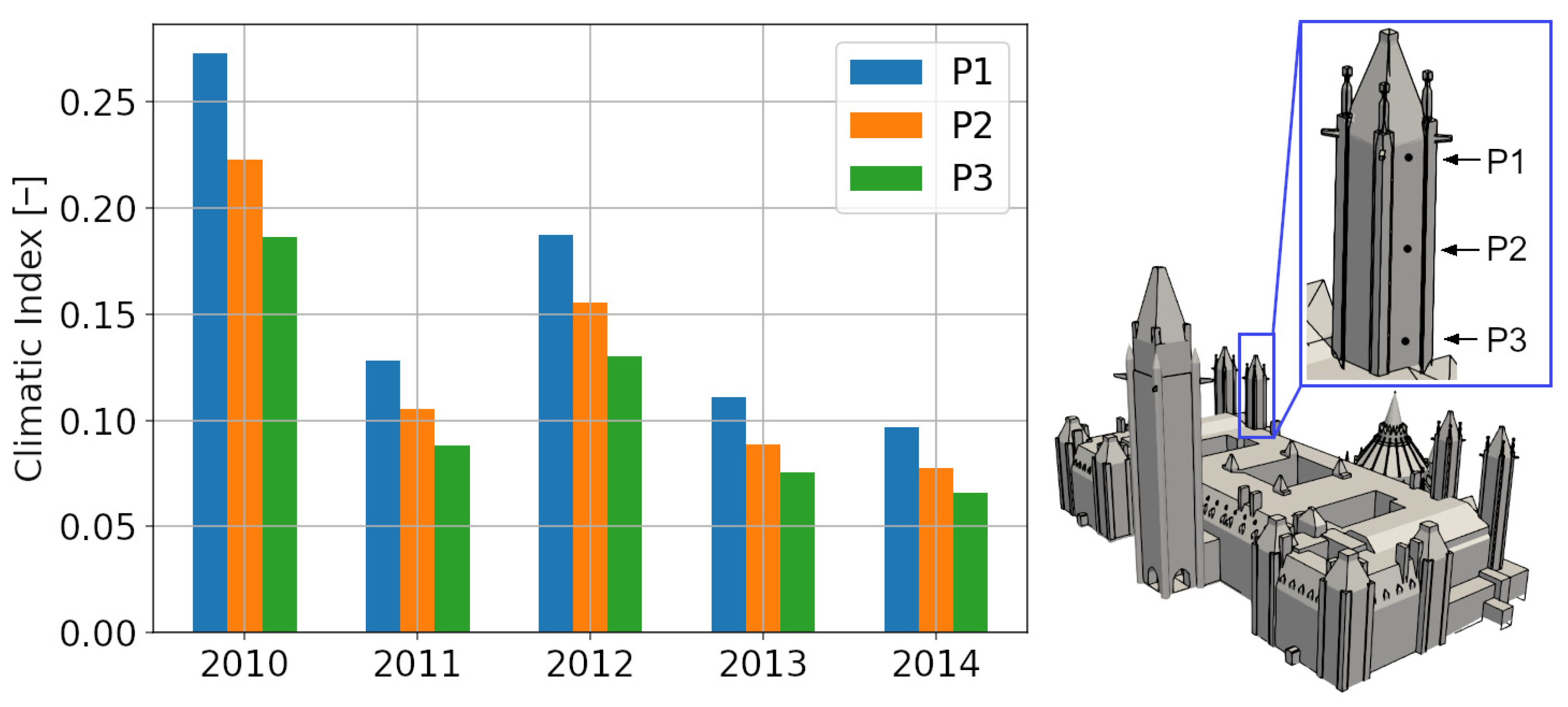
As a first step, the climatic index values are compared in
Figure 9 for each year at the three indicated positions (P1–P3) in the vertical center plane on the east–northeast façade of smaller tower #2. The climatic index is calculated as the annual cumulative WDR at the three positions, obtained from the CFD simulations, divided by the annual cumulative potential evaporation. WDR load can show a large variation between different orientations and years (see free-field WDR values in
Figure 6a) and for different locations on the same façade (
Figure 7c and
Figure 8). In comparison, potential evaporation shows only slight variation across the years (
Figure 6b). Furthermore, it is assumed that the potential evaporation is the same for all surfaces facing the same orientation. As a result, the differences between climatic index values follow a trend similar to the free-field WDR amounts for each year, with 2010 and 2012 being more severe years, mainly due to a larger amount of WDR events from the east–northeast. The values for position P1 are consistently higher, indicating a more severe situation for higher locations on the façade.
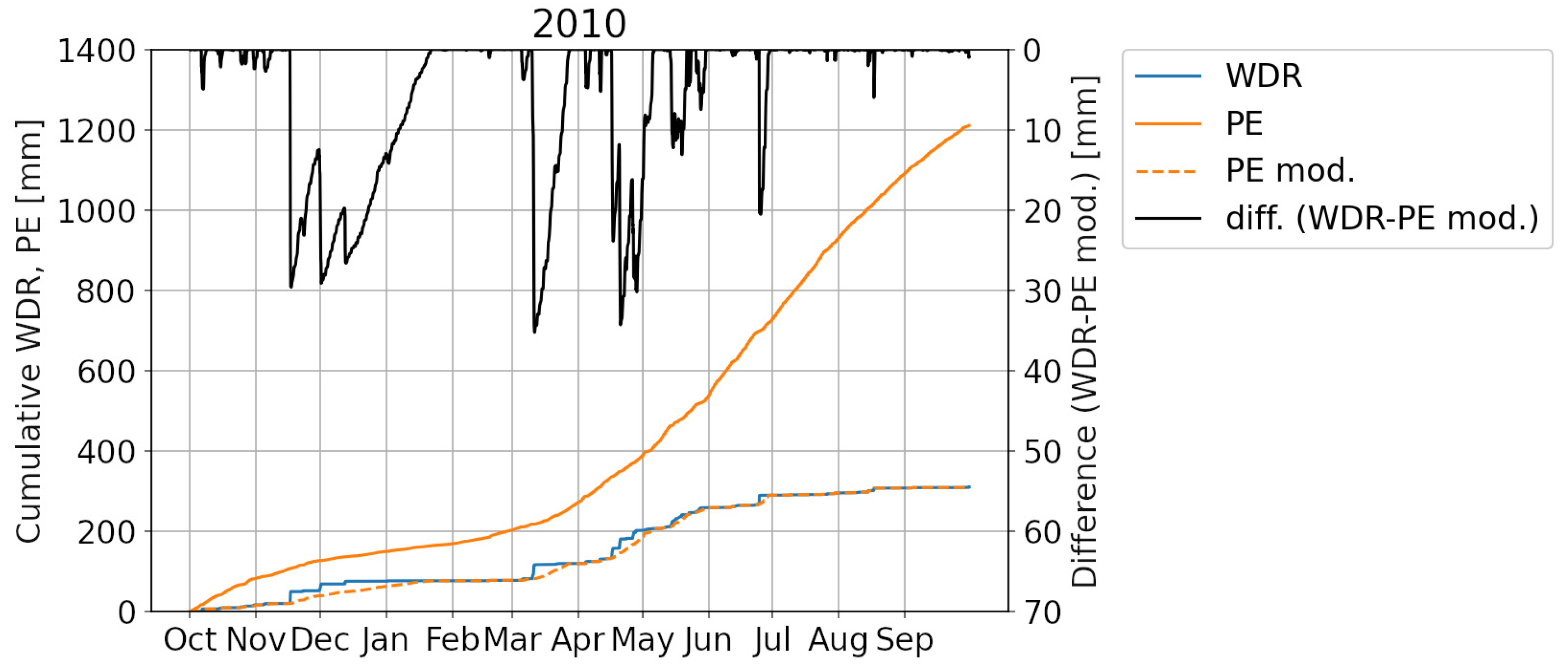
A drawback of the climate index method is that only yearly values of WDR and PE are compared, lacking a time-dependent evaluation of wetting and drying over the year. For example,
Figure 10 shows the cumulative WDR and potential evaporation over time for position P1 during 2010. Potential evaporation is observed to be larger than the total wetting throughout the complete duration. Potential evaporation mainly increases from April to September, and remains rather low starting from October during winter. However, it should be kept in mind that once the absorbed rainwater completely dries out, additional evaporation cannot further reduce the moisture content and, as such, should not be accounted for. Therefore, we propose to determine a modified cumulative potential evaporation curve in
Figure 10, where this evaporation surplus is removed. We observe that, until mid-November, WDR exposure at position P1 is low enough and all moisture by WDR can evaporate. However, once the rain events in mid-November start, a larger amount of moisture is deposited onto the envelope and not all moisture can evaporate. The difference between the cumulative WDR (blue line) and the cumulative modified PE (dashed orange line) is indicated by the black line. This condition continues until around mid-January. Other similar periods with WDR being higher than the modified PE are observed later in spring and summer, with shorter durations. Note again that we assume that all WDR reaching the façade is absorbed by the wall masonry, neglecting splashing, film formation, and runoff.
The potential evaporation gives the maximum amount of water that can evaporate at the exterior surface of the building envelope, independent of materials. One may therefore expect that there will be moisture residing within the building envelope during the periods when the cumulative WDR is larger than the modified cumulative potential evaporation in
Figure 10. In reality, both the actual WDR uptake and the evaporation amount depend on the moisture transport properties of the material. In certain cases, moisture can stay within the envelope while the exterior surface completely dries out. In such cases, the potential evaporation overestimates the drying rate. Furthermore, this approach does not consider heat storage in the envelope. Despite these limitations in determining wetting by WDR and drying by potential evaporation, this method allows a fast first estimate of moisture loadings that could lead to damage risks.
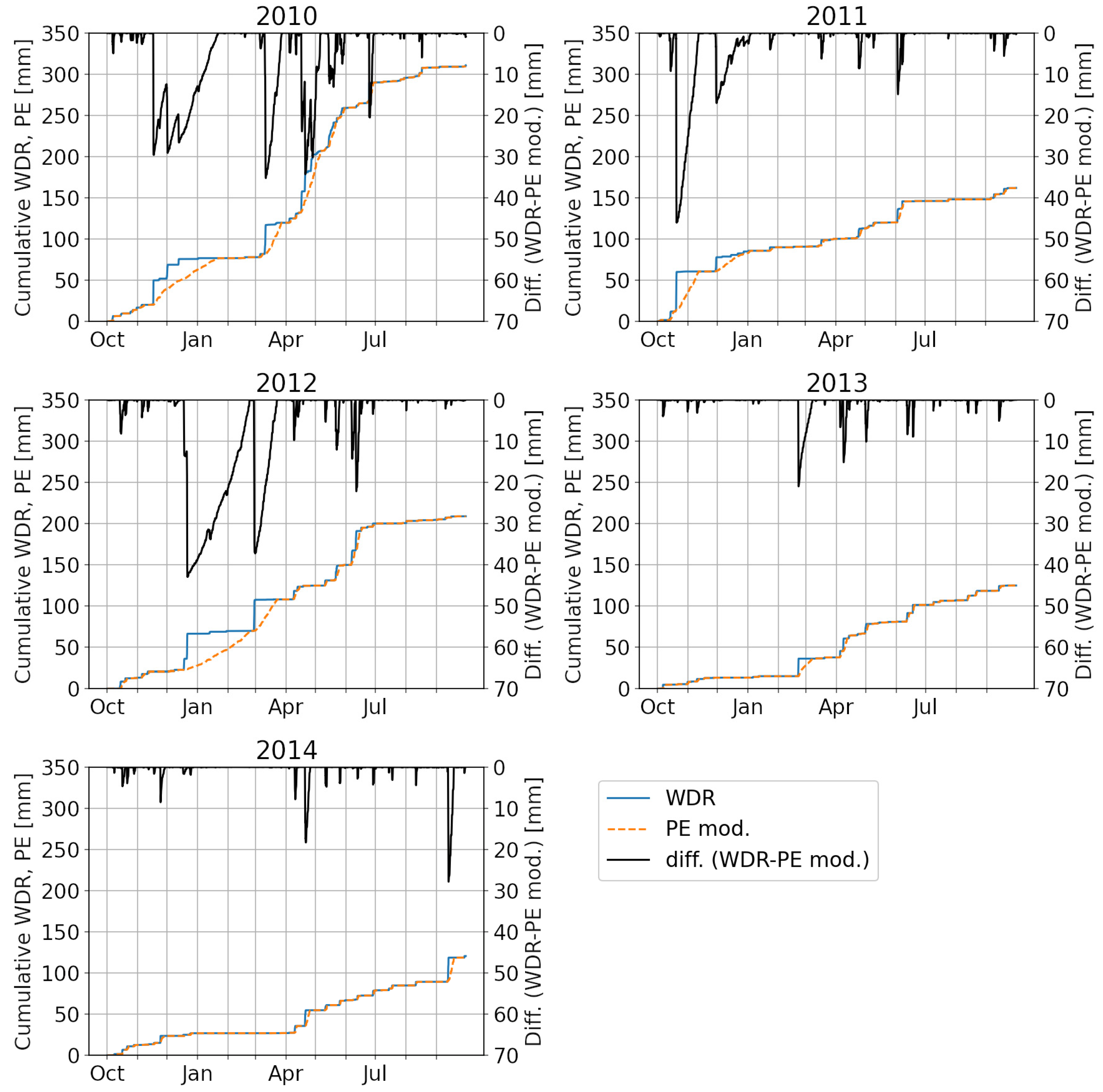
Figure 11 shows the comparison between the modified cumulative potential evaporation and the cumulative WDR for each year separately. There is a significant variation in terms of WDR wetting load across the years. Furthermore, long durations with larger wetting load than potential evaporation are observed in the years 2010–2012. There is also a seasonal variation across the different years in
Figure 11, indicating that moisture can stay in the envelope during long periods in autumn, winter, or spring. The total WDR amount for the orientation east–northeast is the lowest in 2013 and 2014, as shown in
Figure 6a. For these years, the critical periods, where wetting is larger than potential evaporation, are much shorter. We remark that only the wetting due to WDR is taken into account, ignoring precipitation in the form of snow, as it is considered that snow does not cause wetting of façades. Therefore, it is possible that there is additional snowfall during the periods of constant cumulative WDR in
Figure 11.
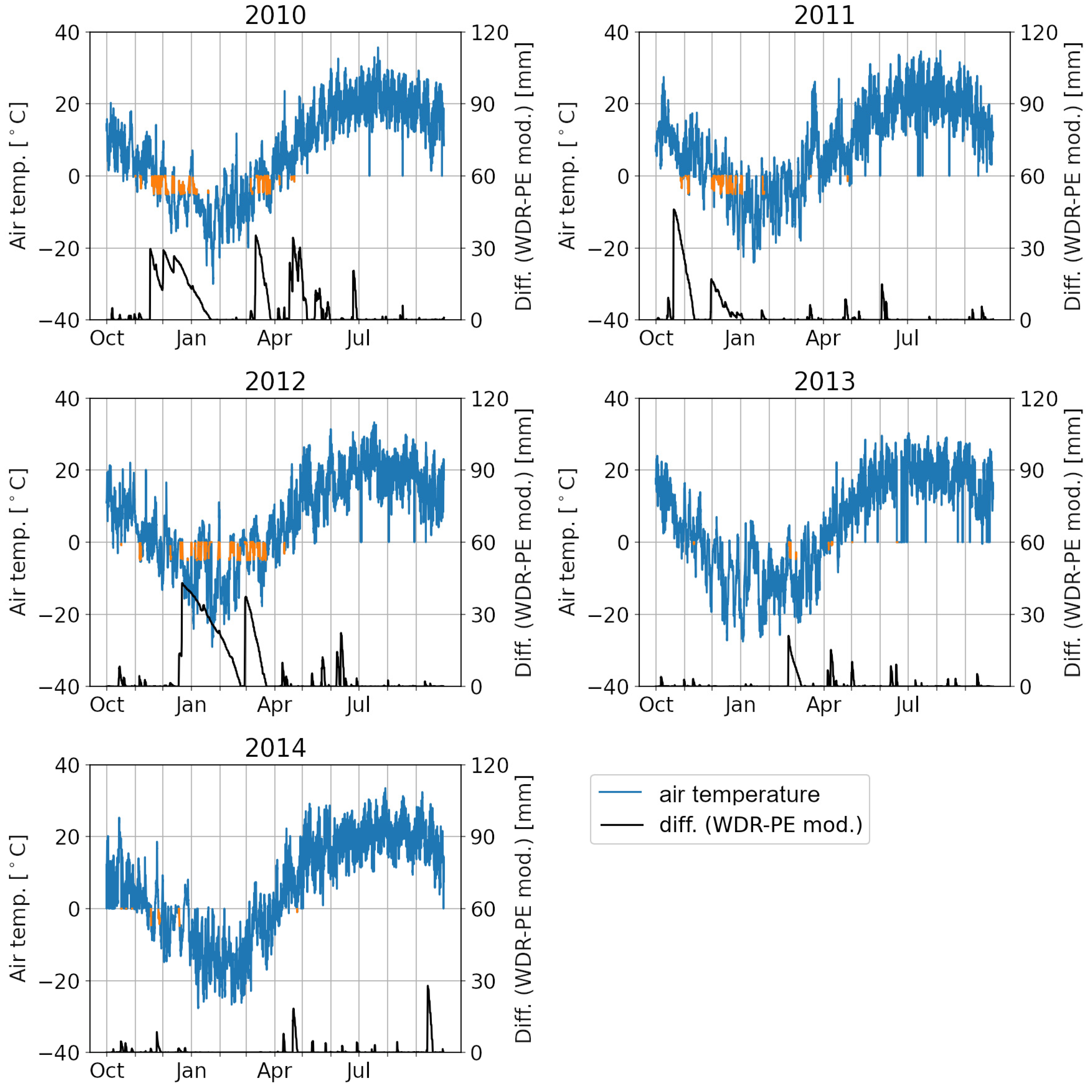
Figure 12 gives the air temperature during the critical periods, where the orange parts indicate that there is moisture inside the envelope at position P1 while air temperature is between −5 °C and 0 °C. We observe that ambient air temperature fluctuates around 0 °C during this critical period, indicating a high risk of freeze–thaw damage. The temperature range between −5 °C and 0 °C is considered, since the freezing temperature of water in porous medium depends on pore size due to freezing-point depression, and water in the smaller pores freezes at temperatures lower than 0 °C [
3,
5,
12]. This means that the parts of the line indicated in orange correspond to the periods with risk of freeze–thaw damage. As expected, the years 2010–2012 show longer periods with risk of such damage. The following subsection discusses how these periods are likely to change in the future considering climate change.
6.3. Impact of Climate Change and Future Climatic Conditions
6.3.1. Description of Weather Morphing
In order to assess the impact of climate change, the current weather data, obtained from measurements, were modified to reflect the potential change in future rain events. Monthly changes in precipitation and air temperature as predicted by the PCIC12 ensemble, provided by the Pacific Climate Impacts Consortium (PCIC), were extracted from the PCIC Climate Explorer tool [
49]. PCIC12 is an ensemble of 12 downscaled global climate models, representing average projected conditions. The statistical information on climate projections was obtained for Ottawa, e.g., current and future mean, maximum, and minimum values of precipitation and air temperature, with standard deviation. As for the future conditions, the RCP8.5 and RCP4.5 scenarios are considered here, assuming the worst case with high emission conditions as well as a moderate case with a peak in emissions.
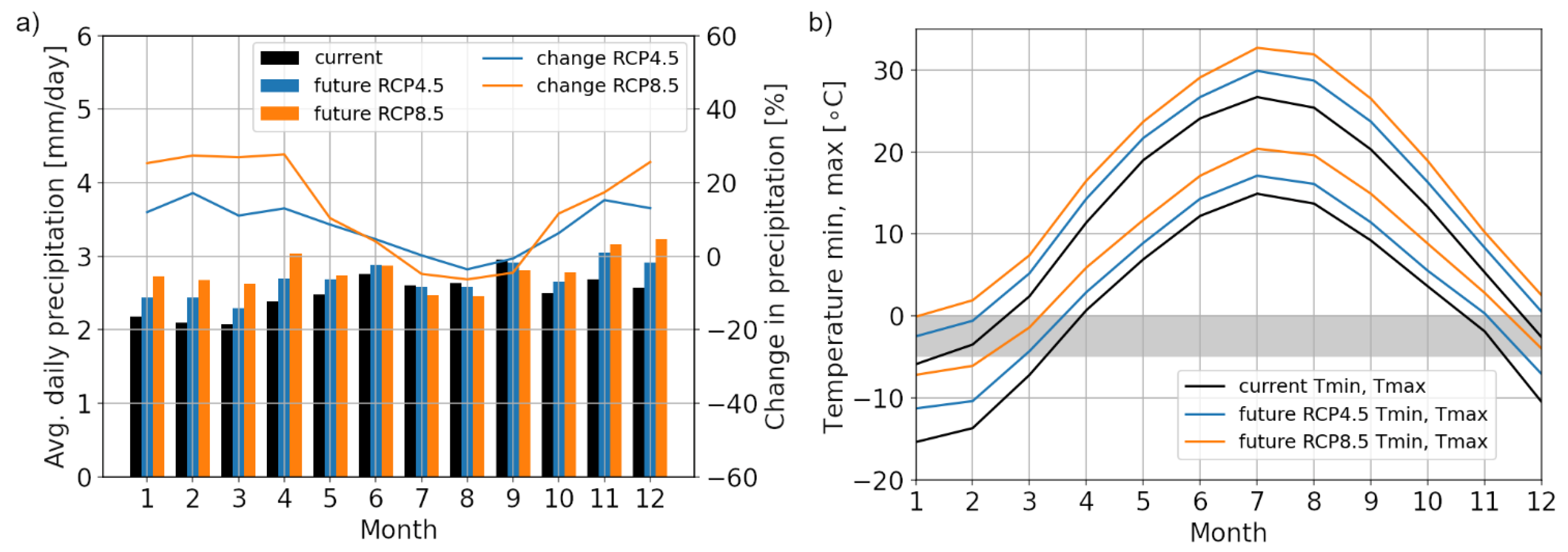
The future precipitation values were obtained by simply scaling the 15 min measured data by the predicted changes for each month, as shown in
Figure 13a. The precipitation levels increase in almost all months except for July, August, and September, where a slight decrease is predicted. The changes are generally larger in the RCP8.5 scenario. Precipitation during winter may increase by up to 27%, while in summer the decrease goes up to 6%.
The range between the monthly minimum and maximum air temperatures is shown in
Figure 13b for the current conditions and future scenarios. The overall air temperature level is increasing, with RCP8.5 leading to a higher rise in temperatures. The temperature shift occurs through the range where freeze–thaw damage is likely, as indicated by the gray box, between −5 °C and 0 °C. The hourly dry-bulb temperature from the measured data was used to obtain the future temperature values based on the “shift and stretch” algorithm explained by Belcher et al. [
16]. This algorithm is convenient for events with a shift in an overall value—e.g., a change in mean air temperature—and with a change within the diurnal cycle, e.g., changes in minimum and maximum air temperatures. The predicted hourly air temperature for the future cases was obtained as follows [
16]:
where
T0 denotes the current hourly measured value, Δ〈
T〉
m the absolute change in the monthly mean temperature, and 〈
T0〉
m the current monthly mean temperature.
αT denotes the fractional change in the monthly mean temperature, and is defined as:
where Δ
Tmax,m and Δ
Tmin,m are the absolute changes in monthly maximum and minimum temperatures, respectively, and
T0max,m and
T0min,m are the current monthly maximum and minimum temperatures, respectively.
Precipitation duration was assumed to remain constant. Furthermore, the effects of climate change on mean wind velocity were assumed to be relatively modest [
3,
50], so no additional modification was made for the wind-flow conditions. We note that the calculated catch ratios for the building can also be used for WDR predictions with climate change, since catch ratios are given as a function of horizontal rain intensity and wind speed for different wind directions.
6.3.2. Comparison of Current and Future Risks of Freeze–Thaw Damage
The potential impact of future climatic conditions on the risk of freeze–thaw damage will result from the combined effects of several parameters:
- (1)
WDR exposure is expected to increase due to climate change. It is predicted that the amount of overall precipitation will increase in the future. At the same time, with increased temperatures in the future, some of the existing snowfall will convert into rainfall, which will further increase the WDR exposure;
- (2)
Higher temperatures in the future will increase potential evaporation, acting in opposition to the increase in WDR exposure;
- (3)
Increases in temperature will cause a shift in the periods during which potential freeze–thaw damage can occur. This means that façades and periods currently showing high risk of freeze–thaw damage may in future no longer be exposed to this type of damage, while façades and periods currently remaining in freezing conditions may, in future, be exposed to freeze–thaw damage.
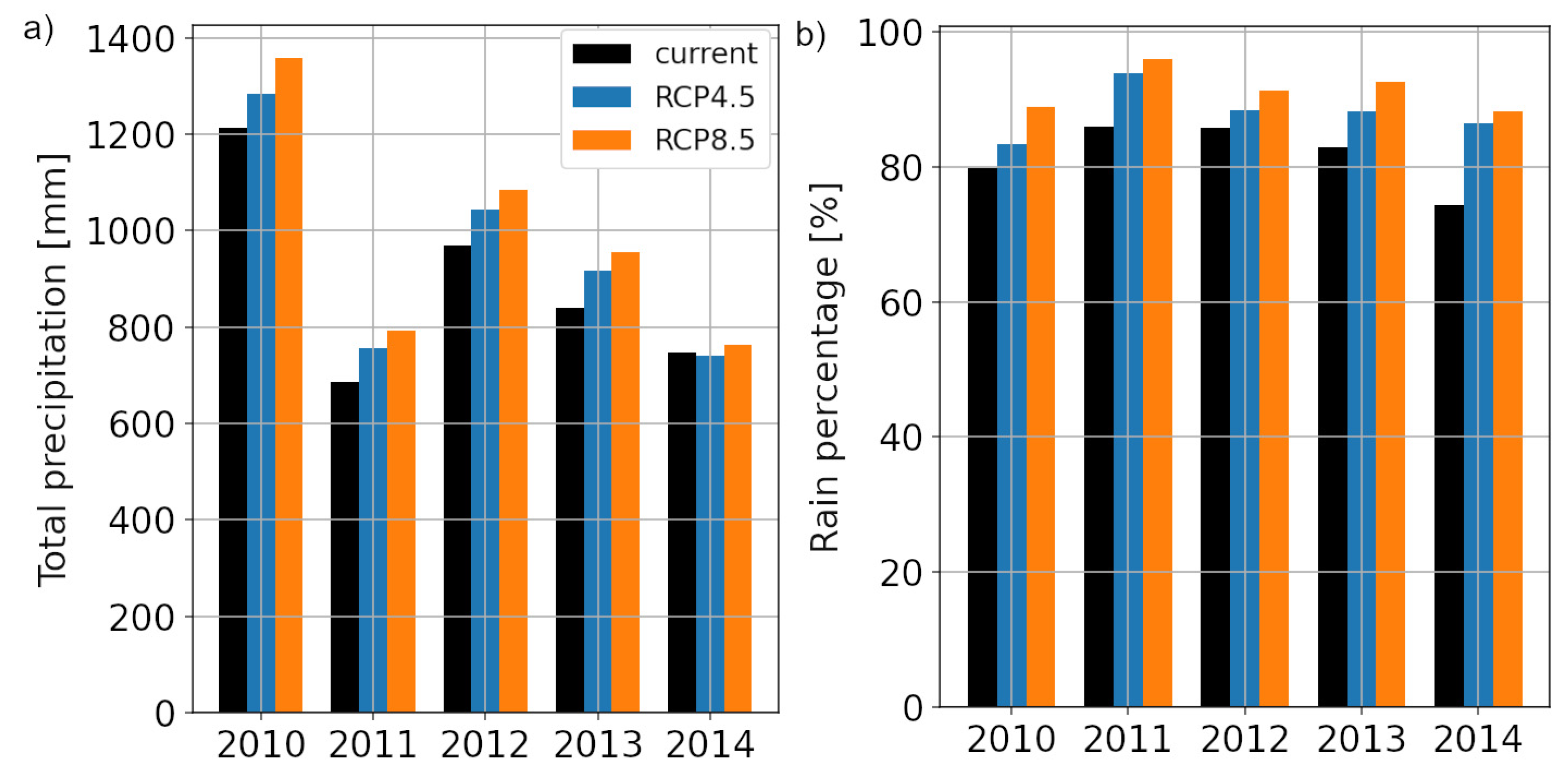
The predicted changes given in
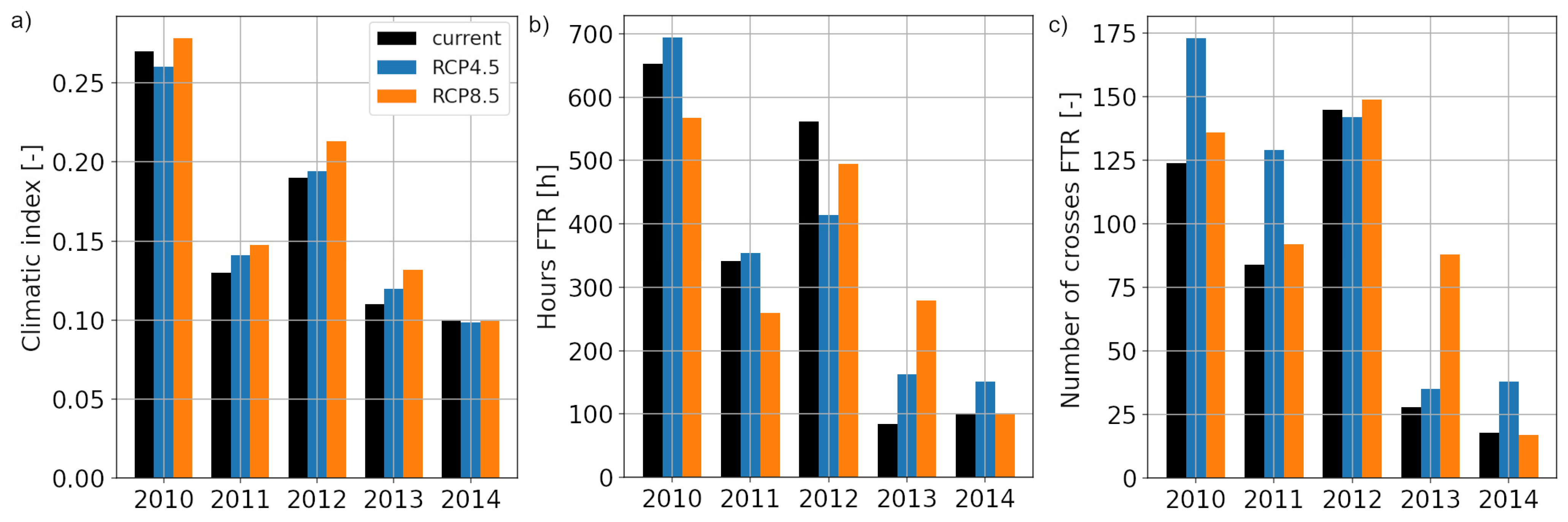
Figure 14 show that both RCP4.5 and RCP8.5 indicate an increase in total rain due to increases in both total precipitation and percentage of rain with increasing temperatures. Overall, climatic index values show an increase in the future in
Figure 15a—especially for RCP8.5—but the difference between the current and future values remains low, indicating that the increases in the annual cumulative values of WDR and potential evaporation are comparable. Note that a higher climatic index does not necessarily indicate a higher risk of freeze–thaw damage. With the predicted conditions in the future, the analyses carried out for the results shown in
Figure 11 and
Figure 12 are repeated for the RCP4.5 and RCP8.5 scenarios for freeze–thaw damage risk.
The change in the freeze–thaw damage risk considering future scenarios is discussed using two indices: First is “the number of hours of freeze–thaw risk”, indicating the total duration of the periods where cumulative WDR is larger than cumulative PE while air temperature is between −5 °C and 0 °C. This is similar to the “time of frost” [
6], and presents a simple indicator given the complex underlying physics of freeze–thaw damage. The number of freeze–thaw cycles is more critical than the total duration between −5 °C and 0 °C, as the damage is related to the resulting mechanical stresses during repeated freezing and thawing. In other words, if temperature remains at the same level between −5 °C and 0 °C, it does not necessarily lead to freeze–thaw damage. The potential for such cycles can be represented by simply counting the number of freeze–thaw cycles [
5], and additionally by taking into account the moisture content in the material [
6,
51]. Here, as a second index, “the number of crossings” across the −5 °C to 0 °C range is considered with the constraint that, concurrently, cumulative WDR is larger than cumulative PE.
In
Figure 15b, the number of hours of freeze–thaw risk shows a trend over the years similar to that of the climatic index. However, the predicted changes differ, largely depending on the conditions during the base year. For both 2010 and 2011, the risk increases for the moderate RCP4.5 scenario, but decreases with a further increase in temperatures with RCP8.5. While the WDR exposure increases in future scenarios for both RCP4.5 and RCP8.5, a larger increase in air temperature in the RCP8.5 scenario causes a reduction in wet periods with temperatures in the range of −5°–0 °C. Inversely, for the conditions in 2013, the freeze–thaw damage risk increases greatly. This is largely because the measured air temperatures in 2013 are comparatively low, and both the occurrence of rain events and the duration between −5 °C and 0 °C increase with climate change.
The number of crossings across the −5 °C to 0 °C range, as shown in
Figure 15c, bears certain similarities to the hours of freeze–thaw risk, with a few minor differences. For 2010 and 2011, both RCP4.5 and RCP8.5 indicate an increase in risk. The main observation that the risk is higher at RCP4.5 than it is at RCP8.5 remains valid. For 2012 and 2014, no large difference is observed while, for 2013, the increase in future freeze–thaw risk is clearer.
7. Discussion
In the present methodology, CFD simulations of WDR are carried out to determine critical locations on the façades of a building of complex geometry. Then, long-term WDR accumulation and potential evaporation are calculated to provide a first estimate of the risk of freeze–thaw damage in a fast manner, based on both historic and future data. Note that it is also possible to calculate WDR load through semi-empirical models, with a loss in spatial resolution in terms of WDR load, and a gain in calculation time. However, semi-empirical models provide WDR parameters only for a limited number of common building geometries. In this case study of a historical building with towers and façade detailing, semi-empirical models would raise significant uncertainties given the complexity of the building.
Both the actual WDR uptake and the evaporation depend on the moisture transport properties of the façade material. The storage and transport of heat and moisture within the building envelope are not resolved in the present study. Instead, only the WDR load and potential evaporation at the exterior surface of the façade are taken into account. The raindrops reaching the façade are assumed to be completely absorbed in the envelope at their deposited locations. This assumption represents the worst-case scenario in terms of wetting flux at the position of the highest WDR load. In reality, the impingement of raindrops at the surface can lead to splashing, bouncing, or spreading, which may modify the actual amount of WDR load or the rate of water uptake. Prediction of such complex droplet physics requires detailed knowledge of surface properties as well as raindrop impact conditions. As the surface reaches capillary saturation, droplet coalescence, film forming, and runoff may occur, leading to a redistribution of WDR load. Numerical modeling of runoff can be performed using the Nusselt solution [
52] or thin-film models [
53], which is beyond the scope of the current study. In addition, the present study considers the maximum potential evaporation over the entire considered period. These two assumptions regarding the wetting and drying fluxes generally correspond to a façade material with high moisture permeability. In reality, moisture can also stay within the envelope while the exterior surface completely dries out.
One of the advantages of the applied method is that it is independent of the actual envelope composition. This method is intended as a first estimate for moisture-induced damage risks, and for comparison of the risks under different meteorological conditions. Therefore, the applied indices for freeze–thaw damage risks act as an indication for how likely the freeze–thaw damage will occur, and how this risk will change over the years. In reality, reaching freezing conditions is not enough for freeze–thaw damage to occur. Additionally, the material should be at a critical degree of saturation of moisture content at the time of freezing, and the internal freezing stresses should be higher than the material strength [
54,
55]. The accurate representation of these mechanisms and direct conclusions on freeze–thaw damage would require a hygrothermal simulation, eventually coupled to a mechanical simulation, which could resolve the occurrence of freezing and thawing locally, considering the pore-size distribution of the material [
12,
56,
57] and the resulting mechanical stresses.
Building damage risks could increase in the coming decades due to climate change, reinforcing the need for accurate information on the spatial and temporal distribution of WDR. Further work is planned to perform hygrothermal simulations for those specific locations selected from CFD analyses, and for the critical periods based on the climatic indices. In this paper, we show that the choice of reference year has an impact on the evaluation of the risk of freeze–thaw damage, which is very sensitive to temperature. Further work is needed in order to develop a methodology to select a reference year, or a range of reference years, for evaluating the impact of climate change.
8. Conclusions
Detailed CFD simulations of the wind-flow field were performed around the Parliament buildings in Ottawa, Canada. The calculated time-varying WDR load was combined with the time-varying potential evaporation. The combined approach of CFD with wetting and drying fluxes helps to locate critical zones with high WDR load, and to provide a first assessment of the moisture-induced damage risk over the course of several years. Based on the CFD simulations, the highest WDR exposure on the Center Block was observed on the smaller towers, which cause a limited disturbance to the approaching wind flow, i.e., lower wind blockage. Additionally, the corners of the main tower and the main building have relatively higher WDR exposure.
The results indicate a varying degree of freeze–thaw damage risk over the five years considered. With climate change, the increases in annual rainfall and temperature can have opposite effects in terms of freeze–thaw damage risk. While the façades will be exposed to more WDR in general in the future, freeze–thaw damage risk may increase or decrease, depending on future temperature levels. This is best observed for the 2010 and 2011 conditions, which indicate an increase in freeze–thaw damage risk at moderate increases in temperatures, but a decrease at larger increase in temperatures. For years with lower temperature—e.g., 2013—both moderate and large increases in temperatures indicate a higher risk of freeze–thaw damage in the future. Based on the current measured data, the risky periods are located between November and January, and occasionally also in March. Future predictions show an increasing shift in average temperatures, which will also likely shift the risky periods for freeze–thaw damage. There is a need to develop a methodology for future scenarios that is less sensitive to the choice of reference years. Definitive conclusions with regard to freeze–thaw damage would require detailed hygrothermal simulations of building envelopes, taking into account the critical degree of saturation of the material and the mechanical stresses occurring within the material during freeze–thaw cycles. The presented fast methodology yields estimates, indicating whether a more detailed analysis is required or not, upon which subsequent steps of analysis can be defined.
Author Contributions
Conceptualization: A.K., J.B., J.C. and D.D.; formal analysis: A.K., J.B. and J.G.; methodology: A.K., J.B. and X.Z.; visualization: A.K., J.B. and J.G.; supervision: A.K., J.C. and D.D.; writing—original draft: A.K. and J.B.; writing—review and editing: X.Z., T.V.M., M.A.L., J.C. and D.D. All authors have read and agreed to the published version of the manuscript.
Funding
This research project is supported by the Swiss National Science Foundation (SNF)-Project No. 200021_169323 and the ETH Research Grant ETH-08 16-2. Bourcet acknowledges support by the ETH Foundation through the Excellence Scholarship & Opportunity Programme. Derome acknowledges funding from NSERC Discovery and Canada Research Chair programs.
Acknowledgments
The authors would like to thank Carleton University Library, Ottawa, Canada, for providing GIS LiDAR data and Climate Ontario, Meteorological Service of Canada, for providing measured weather data.
Conflicts of Interest
The authors declare no conflict of interest.
References
- Zhou, X.; Derome, D.; Carmeliet, J. Robust Moisture Reference Year Methodology for Hygrothermal Simulations. Build. Environ. 2016, 110, 23–35. [Google Scholar] [CrossRef]
- Blocken, B.; Carmeliet, J. A Review of Wind-Driven Rain Research in Building Science. J. Wind Eng. Ind. Aerodyn. 2004, 92, 1079–1130. [Google Scholar] [CrossRef]
- Vandemeulebroucke, I.; Defo, M.; Lacasse, M.A.; Caluwaerts, S.; Van Den Bossche, N. Canadian Initial-Condition Climate Ensemble: Hygrothermal Simulation on Wood-Stud and Retrofitted Historical Masonry. Build. Environ. 2021, 187, 107318. [Google Scholar] [CrossRef]
- Cornick, S.; Djebbar, R.; Alan Dalgliesh, W. Selecting Moisture Reference Years Using a Moisture Index Approach. Build. Environ. 2003, 38, 1367–1379. [Google Scholar] [CrossRef]
- Grossi, C.M.; Brimblecombe, P.; Harris, I. Predicting Long Term Freeze–Thaw Risks on Europe Built Heritage and Archaeological Sites in a Changing Climate. Sci. Total Environ. 2007, 377, 273–281. [Google Scholar] [CrossRef]
- Kočí, J.; Maděra, J.; Keppert, M.; Černý, R. Damage Functions for the Cold Regions and Their Applications in Hygrothermal Simulations of Different Types of Building Structures. Cold Reg. Sci. Technol. 2017, 135, 1–7. [Google Scholar] [CrossRef]
- Brimblecombe, P.; Grossi, C.M.; Harris, I. Climate Change Critical to Cultural Heritage. In Survival and Sustainability: Environmental Concerns in the 21st Century; Gökçekus, H., Türker, U., LaMoreaux, J.W., Eds.; Springer: Berlin/Heidelberg, Germany, 2011; pp. 195–205. ISBN 978-3-540-95991-5. [Google Scholar]
- Hukka, A.; Viitanen, H.A. A Mathematical Model of Mould Growth on Wooden Material. Wood Sci. Technol. 1999, 33, 475–485. [Google Scholar] [CrossRef]
- Mukhopadhyaya, P.; Kumaran, K.; Tariku, F.; van Reenen, D. Application of Hygrothermal Modeling Tool to Assess Moisture Response of Exterior Walls. J. Archit. Eng. 2006, 12, 178–186. [Google Scholar] [CrossRef]
- Al-Omari, A.; Beck, K.; Brunetaud, X.; Török, Á.; Al-Mukhtar, M. Critical Degree of Saturation: A Control Factor of Freeze–Thaw Damage of Porous Limestones at Castle of Chambord, France. Eng. Geol. 2015, 185, 71–80. [Google Scholar] [CrossRef]
- Calle, K.; Van Den Bossche, N. Analysis of Different Frost Indexes and Their Potential to Assess Frost Based on HAM Simulations. In Proceedings of the 14th International Conference on Durability of Building Materials and Components (XIV DBMC), Ghent, Belgium, 29–31 May 2017. [Google Scholar]
- Zhou, X.; Derome, D.; Carmeliet, J. Hygrothermal Modeling and Evaluation of Freeze-Thaw Damage Risk of Masonry Walls Retrofitted with Internal Insulation. Build. Environ. 2017, 125, 285–298. [Google Scholar] [CrossRef]
- Nik, V.M.; Sasic Kalagasidis, A.; Kjellström, E. Assessment of Hygrothermal Performance and Mould Growth Risk in Ventilated Attics in Respect to Possible Climate Changes in Sweden. Build. Environ. 2012, 55, 96–109. [Google Scholar] [CrossRef]
- Sehizadeh, A.; Ge, H. Impact of Future Climates on the Durability of Typical Residential Wall Assemblies Retrofitted to the PassiveHaus for the Eastern Canada Region. Build. Environ. 2016, 97, 111–125. [Google Scholar] [CrossRef]
- Zhou, X.; Carmeliet, J.; Derome, D. Assessment of Risk of Freeze-Thaw Damage in Internally Insulated Masonry in a Changing Climate. Build. Environ. 2020, 175, 106773. [Google Scholar] [CrossRef]
- Belcher, S.; Hacker, J.; Powell, D. Constructing Design Weather Data for Future Climates. Build. Serv. Eng. Res. Technol. 2005, 26, 49–61. [Google Scholar] [CrossRef]
- Gaur, A.; Lacasse, M.; Armstrong, M. Climate Data to Undertake Hygrothermal and Whole Building Simulations Under Projected Climate Change Influences for 11 Canadian Cities. Data 2019, 4, 72. [Google Scholar] [CrossRef]
- Blocken, B.; Abuku, M.; Nore, K.; Briggen, P.M.; Schellen, H.L.; Thue, J.V.; Roels, S.; Carmeliet, J. Intercomparison of Wind-Driven Rain Deposition Models Based on Two Case Studies with Full-Scale Measurements. J. Wind Eng. Ind. Aerodyn. 2011, 99, 448–459. [Google Scholar] [CrossRef][Green Version]
- Freitas, S.; Barreira, E.; De Freitas, V.P. Quantification of Wind-Driven Rain and Evaluation of Façade Humidification. In Proceedings of the 2nd Central European Symposium on Building Physics (CESBP 2013), Vienna, Austria, 9–11 September 2013. [Google Scholar]
- Kubilay, A.; Derome, D.; Blocken, B.; Carmeliet, J. High-Resolution Field Measurements of Wind-Driven Rain on an Array of Low-Rise Cubic Buildings. Build. Environ. 2014, 78, 1–13. [Google Scholar] [CrossRef]
- Unsplash Photo by Benoit Debaix on Unsplash. Available online: https://unsplash.com/photos/ReUoz0CwfGo (accessed on 21 July 2021).
- Parliament Hill from a Hot Air Balloon. Available online: https://en.wikipedia.org/w/index.php?title=File:Parliament_Hill_from_a_Hot_Air_Balloon,_Ottawa,_Ontario,_Canada,_Y2K_(7173715788).jpg (accessed on 7 August 2021).
- Shih, T.-H.; Liou, W.W.; Shabbir, A.; Yang, Z.; Zhu, J. A New K-ϵ Eddy Viscosity Model for High Reynolds Number Turbulent Flows. Comput. Fluids 1995, 24, 227–238. [Google Scholar] [CrossRef]
- Huang, S.H.; Li, Q.S. Numerical Simulations of Wind-Driven Rain on Building Envelopes Based on Eulerian Multiphase Model. J. Wind Eng. Ind. Aerodyn. 2010, 98, 843–857. [Google Scholar] [CrossRef]
- Kubilay, A.; Derome, D.; Blocken, B.; Carmeliet, J. CFD Simulation and Validation of Wind-Driven Rain on a Building Facade with an Eulerian Multiphase Model. Build. Environ. 2013, 61, 69–81. [Google Scholar] [CrossRef]
- Kubilay, A.; Derome, D.; Blocken, B.; Carmeliet, J. Numerical Simulations of Wind-Driven Rain on an Array of Low-Rise Cubic Buildings and Validation by Field Measurements. Build. Environ. 2014, 81, 283–295. [Google Scholar] [CrossRef]
- Kubilay, A.; Derome, D.; Blocken, B.; Carmeliet, J. Wind-Driven Rain on Two Parallel Wide Buildings: Field Measurements and CFD Simulations. J. Wind Eng. Ind. Aerodyn. 2015, 146, 11–28. [Google Scholar] [CrossRef]
- Gunn, R.; Kinzer, G.D. The Terminal Velocity of Fall for Water Droplets in Stagnant Air. J. Meteorol. 1949, 6, 243–248. [Google Scholar] [CrossRef]
- Kubilay, A.; Derome, D.; Blocken, B.; Carmeliet, J. Numerical Modeling of Turbulent Dispersion for Wind-Driven Rain on Building Facades. Environ. Fluid Mech. 2015, 15, 109–133. [Google Scholar] [CrossRef]
- WindDrivenRainFoam—An Open-Source Solver for Wind-Driven Rain Based on OpenFOAM. Available online: https://gitlab.ethz.ch/openfoam-cbp/solvers/winddrivenrainfoam (accessed on 8 July 2021).
- Best, A.C. The Size Distribution of Raindrops. Q. J. R. Meteorol. Soc. 1950, 76, 16–36. [Google Scholar] [CrossRef]
- Blocken, B.; Carmeliet, J. High-Resolution Wind-Driven Rain Measurements on a Low-Rise Building—Experimental Data for Model Development and Model Validation. J. Wind Eng. Ind. Aerodyn. 2005, 93, 905–928. [Google Scholar] [CrossRef]
- Ge, H.; Deb Nath, U.K.; Chiu, V. Field Measurements of Wind-Driven Rain on Mid-and High-Rise Buildings in Three Canadian Regions. Build. Environ. 2017, 116, 228–245. [Google Scholar] [CrossRef]
- Blocken, B.; Carmeliet, J. Spatial and Temporal Distribution of Driving Rain on a Low-Rise Building. Wind Struct. 2002, 5, 441–462. [Google Scholar] [CrossRef]
- Penman, H.L. Natural Evaporation from Open Water, Bare Soil and Grass. Proc. R. Soc. Lond. Ser. Math. Phys. Sci. 1948, 193, 120–145. [Google Scholar] [CrossRef]
- Allen, R.G.; Pereira, L.S.; Raes, D.; Smith, M. Crop Evapotranspiration-Guidelines for Computing Crop Water Requirements-FAO Irrigation and Drainage Paper 56; Food and Agriculture Organization of the United Nations: Rome, Italy, 1998; Volume 9, p. D05109. [Google Scholar]
- Ottawa LiDAR|MacOdrum Library. Available online: https://library.carleton.ca/find/gis/geospatial-data/ottawa-lidar (accessed on 3 July 2021).
- City of London Corporation. Wind Microclimate Guidelines for Developments in the City of London; City of London Corporation: London, UK, 2019. [Google Scholar]
- Franke, J.; Hellsten, A.; Schlünzen, H.; Carissimo, B. (Eds.) Best Practice Guideline for the CFD Simulation of Flows in the Urban Environment: COST Action 732: Quality Assurance and Improvement of Microscale Meteorological Models; COST Office: Brussels, Belguim, 2007; ISBN 3-00-018312-4. [Google Scholar]
- Azevedo, J.M.S. Development of Procedures for the Simulation of Atmospheric Flows over Complex Terrain, Using OpenFOAM. Master’s Thesis, Instituto Politécnico do Porto, Instituto Superior de Engenharia do Porto, Porto, Portugal, 2013. [Google Scholar]
- Disura|3D Warehouse. Available online: https://3dwarehouse.sketchup.com/user/0010152151449342952439405/Disura?filter=parliament%20block (accessed on 3 August 2021).
- Kubilay, A.; Carmeliet, J.; Derome, D. Computational Fluid Dynamics Simulations of Wind-Driven Rain on a Mid-Rise Residential Building with Various Types of Facade Details. J. Build. Perform. Simul. 2017, 10, 125–143. [Google Scholar] [CrossRef]
- Briggen, P.M.; Blocken, B.; Schellen, H.L. Wind-Driven Rain on the Facade of a Monumental Tower: Numerical Simulation, Full-Scale Validation and Sensitivity Analysis. Build. Environ. 2009, 44, 1675–1690. [Google Scholar] [CrossRef]
- ESRI Basemap City of Ottawa LiDAR Index (Sources: City of Ottawa, Ville de Gatineau, Province of Ontario, Esri Canada, Esri, HERE, Garmin, INCREMENT P, Intermap, USGS, METI/NASA, EPA, USDA, AAFC, NRCan). 2018. Available online: https://www.arcgis.com/home/item.html?id=bb86c9b09c7f4e03a061badaf7464245 (accessed on 7 March 2021).
- Bourcet, J. Simulation of Wind-Driven Rain Exposure and Hygrothermal Analysis of Heritage Façades Using Future Climate Weather Data. Master’s Thesis, ETH Zurich, Zürich, Switzerland, 2020. [Google Scholar]
- Richards, P.J.; Hoxey, R.P. Appropriate Boundary Conditions for Computational Wind Engineering Models Using the K-E Turbulence Model. J. Wind Eng. Ind. Aerodyn. 1993, 46–47, 145–153. [Google Scholar] [CrossRef]
- Blocken, B.; Carmeliet, J. Overview of Three State-of-the-Art Wind-Driven Rain Assessment Models and Comparison Based on Model Theory. Build. Environ. 2010, 45, 691–703. [Google Scholar] [CrossRef]
- Lacy, R.E. Climate and Building in Britain: A Review of Meteorological Information Suitable for Use in the Planning, Design, Construction, and Operation of Buildings (Building Research Establishment Report); H.M. Stationery Off: London, UK, 1977. [Google Scholar]
- PCIC Climate Explorer. Available online: https://services.pacificclimate.org/pcex/app/#/data/climo/ce_files (accessed on 9 March 2021).
- Cheng, C.S.; Li, G.; Li, Q.; Auld, H.; Fu, C. Possible Impacts of Climate Change on Wind Gusts under Downscaled Future Climate Conditions over Ontario, Canada. J. Clim. 2012, 25, 3390–3408. [Google Scholar] [CrossRef]
- Lisø, K.R.; Kvande, T.; Hygen, H.O.; Thue, J.V.; Harstveit, K. A Frost Decay Exposure Index for Porous, Mineral Building Materials. Build. Environ. 2007, 42, 3547–3555. [Google Scholar] [CrossRef]
- Blocken, B.; Carmeliet, J. A Simplified Numerical Model for Rainwater Runoff on Building Facades: Possibilities and Limitations. Build. Environ. 2012, 53, 59–73. [Google Scholar] [CrossRef]
- Martin, M.; Defraeye, T.; Derome, D.; Carmeliet, J. A Film Flow Model for Analysing Gravity-Driven, Thin Wavy Fluid Films. Int. J. Multiph. Flow 2015, 73, 207–216. [Google Scholar] [CrossRef]
- Straube, J.; Schumacher, C.; Mensinga, P. Assessing the Freeze-Thaw Resistance of Clay Brick for Interior Insulation Retrofit Projects. In Proceedings of the Proceedings of the XI International Conference Thermal Performance of the Exterior Envelopes of Whole Buildings., Clearwater, FL, USA, 5–9 December 2010. [Google Scholar]
- van Aarle, M.; Schellen, H.; van Schijndel, J. Hygro Thermal Simulation to Predict the Risk of Frost Damage in Masonry; Effects of Climate Change. Energy Procedia 2015, 78, 2536–2541. [Google Scholar] [CrossRef]
- Gawin, D.; Pesavento, F.; Koniorczyk, M.; Schrefler, B.A. Non-Equilibrium Modeling Hysteresis of Water Freezing: Ice Thawing in Partially Saturated Porous Building Materials. J. Build. Phys. 2019, 43, 61–98. [Google Scholar] [CrossRef]
- Calle, K.; Van Den Bossche, N. Sensitivity Analysis of the Hygrothermal Behaviour of Homogeneous Masonry Constructions: Interior Insulation, Rainwater Infiltration and Hydrophobic Treatment. J. Build. Phys. 2021, 44, 510–538. [Google Scholar] [CrossRef]
Figure 1.
Views of (
a) the Center Block of the Parliament buildings from the south (Photo by Benoit Debaix [
21]), and (
b) Parliament Hill from north (Photo by tsaiproject [
22]/CC-BY-2.0).
Figure 1.
Views of (
a) the Center Block of the Parliament buildings from the south (Photo by Benoit Debaix [
21]), and (
b) Parliament Hill from north (Photo by tsaiproject [
22]/CC-BY-2.0).
Figure 2.
(
a) Surroundings of Parliament Hill and the extent of the computational domain [
44]. (
b) View of the computational domain showing the terrain and the explicitly-modeled buildings, and (
c) computational grid on the surfaces of the Center Block and the ground. MT denotes the main tower and ST the smaller towers on the Center Block.
Figure 3.
Wind rose (a) for all hourly data in the years 2010–2020, and (b) for conditions with rain.
Figure 3.
Wind rose (a) for all hourly data in the years 2010–2020, and (b) for conditions with rain.
Figure 4.
Histogram of (a) wind speed during rain events, and (b) rainfall intensity based on hourly data in the years 2010–2020.
Figure 4.
Histogram of (a) wind speed during rain events, and (b) rainfall intensity based on hourly data in the years 2010–2020.
Figure 5.
Comparison of annual precipitation and rainfall in the years 2010–2014, obtained from weather station data.
Figure 5.
Comparison of annual precipitation and rainfall in the years 2010–2014, obtained from weather station data.
Figure 6.
(a) Free-field wind-driven rain amount (mm) and (b) potential evaporation (mm) for different façade orientations based on the measured data in the years 2010–2014.
Figure 6.
(a) Free-field wind-driven rain amount (mm) and (b) potential evaporation (mm) for different façade orientations based on the measured data in the years 2010–2014.
Figure 7.
(a) Normalized magnitude of wind velocity at 10 m height for wind approaching from the east; (b) trajectories of 1 mm raindrops reaching the Center Block (CB) at a reference wind speed, Uref, of 10 m/s; and (c) the corresponding distribution of catch ratio on the CB for a wind speed of 10 m/s and a rainfall intensity of 1 mm/h.
Figure 8.
Catch ratio distribution representing the wetting in 2010 on the façades of smaller tower #2.
Figure 8.
Catch ratio distribution representing the wetting in 2010 on the façades of smaller tower #2.
Figure 9.
Comparison of the climatic index values at the three selected positions on the east–northeast façade of smaller tower #2 (ST2) in the years 2010–2014.
Figure 9.
Comparison of the climatic index values at the three selected positions on the east–northeast façade of smaller tower #2 (ST2) in the years 2010–2014.
Figure 10.
Comparison of the cumulative wind-driven rain and potential evaporation at position P1 during the year 2010. The difference between the two is indicated by the black line.
Figure 10.
Comparison of the cumulative wind-driven rain and potential evaporation at position P1 during the year 2010. The difference between the two is indicated by the black line.
Figure 11.
Comparison of the cumulative wind-driven rain and the modified cumulative potential evaporation in the years 2010–2014. The difference between the two is indicated by the black line.
Figure 11.
Comparison of the cumulative wind-driven rain and the modified cumulative potential evaporation in the years 2010–2014. The difference between the two is indicated by the black line.
Figure 12.
Annual variation in air temperature in the years 2010–2014. Orange parts indicate coincidence of moisture present in the envelope at position P1 and air temperature between −5 °C and 0 °C.
Figure 12.
Annual variation in air temperature in the years 2010–2014. Orange parts indicate coincidence of moisture present in the envelope at position P1 and air temperature between −5 °C and 0 °C.
Figure 13.
(
a) Predicted average daily precipitation and percentage change from current (baseline) values. (
b) Predicted minimum and maximum air temperature for current (baseline) and future conditions [
49].
Figure 13.
(
a) Predicted average daily precipitation and percentage change from current (baseline) values. (
b) Predicted minimum and maximum air temperature for current (baseline) and future conditions [
49].
Figure 14.
Comparison of (a) precipitation and (b) percentage of rain over total precipitation between current conditions and future conditions, based on the RCP4.5 and RCP8.5 scenarios.
Figure 14.
Comparison of (a) precipitation and (b) percentage of rain over total precipitation between current conditions and future conditions, based on the RCP4.5 and RCP8.5 scenarios.
Figure 15.
Comparison of (a) climatic index, (b) hours of freeze–thaw risk, and (c) number of crossings of freeze–thaw risk between current and future conditions, based on the RCP4.5 and RCP8.5 scenarios.
Figure 15.
Comparison of (a) climatic index, (b) hours of freeze–thaw risk, and (c) number of crossings of freeze–thaw risk between current and future conditions, based on the RCP4.5 and RCP8.5 scenarios.
| Publisher’s Note: MDPI stays neutral with regard to jurisdictional claims in published maps and institutional affiliations. |
© 2021 by the authors. Licensee MDPI, Basel, Switzerland. This article is an open access article distributed under the terms and conditions of the Creative Commons Attribution (CC BY) license (https://creativecommons.org/licenses/by/4.0/).


 ,
, 


